Single or Multiple Frames Content Delivery for Next-Generation Networks?
Abstract
This paper addresses the four enabling technologies, namely multi-user sparse code multiple access (SCMA), content caching, energy harvesting, and physical layer security for
proposing an energy and spectral efficient resource allocation algorithm for the access and backhaul links in heterogeneous cellular networks. Although each of the above mentioned issues could be a topic of research, in a real situation, we would face a complicated scenario where they should be considered jointly, and hence, our target is to consider these technologies jointly in a unified
framework. Moreover, we propose two novel content delivery scenarios: 1) single frame content delivery (SFCD), and 2) multiple frames content delivery (MFCD), where the time duration of serving user requests is divided into several frames. In the first scenario, the requested content by each user is served over one frame. However, in the second scenario, the requested content by each user can be delivered over several frames. We formulate the resource allocation for the proposed scenarios as optimization problems where our main aim is to maximize the energy efficiency of access links subject to the transmit power and rate constraints of access and backhaul links, caching and energy harvesting constraints, and SCMA codebook allocation limitations. Due to the practical limitations, we assume that the channel state information values between eavesdroppers and base stations are uncertain and design the network for the worst case scenario. Since the corresponding optimization problems are mixed integer non-linear and nonconvex programming, NP-hard, and intractable, we propose an iterative algorithm based on the well-known alternate and successive convex approximation methods. In addition, the proposed algorithms are studied from the computational complexity, convergence, and performance perspectives. Moreover, the proposed caching scheme outperforms the existing traditional caching schemes like random caching and most popular caching. We also study the effect of joint and disjoint considerations of enabling technologies for the performance of next-generation networks. We also show that the proposed caching strategy, MFCD and joint solutions have 43%, 9.4% and %51.3 performance gain compared to no cahcing, SFCD and disjoint solutions, respectively.
Index Terms– Heterogeneous cellular networks, Content caching, Physical layer security, Energy harvesting, Imperfect CSI.
I Introduction
I-A Background and Motivation
Over recent years, the growth of high data rate of mobile traffic, energy, content storing, security, and limited knowledge of channels over mobile networks are the major challenges of network design and implementation. To tackle these issues and cope with the users’ requirements, the next-generation of wireless communications is introduced which uses multiple advanced techniques such as energy harvesting (EH), physical layer (PHY) security, new multiple access techniques, and content caching. Hence, all of these issues must be considered together and efficient joint radio resource allocation and content placement algorithms must be applied to provide high performance for the designed networks. However, devising efficient algorithms to handle all these issues is a challenging task, and to the best our knowledge, no research exists addressing all these issues together in a unified framework. Although each of the mentioned issues could be an interesting research topic, our main contribution is to study the joint effect of security, EH, content caching, and imperfect and limited channel knowledge in a unified joint access and backhaul links framework. In this regards, we develop a comprehensive model and mathematical representation, and design a robust resource allocation algorithm. Although the resulting optimization problem is complicated, effective optimization methods are used to achieve the solution. The outline of each issue, applicable solutions, and related works are explained in the sequel.
I-A1 Growth of High Data Rate Mobile Traffic
Incredible growth in high data rate mobile applications requires high capacity in radio access and backhaul wireless links. However, the centralized nature of mobile network architectures can not provide enough capacity on the wireless access and backhaul links to satisfy high demand for rich multimedia content. Heterogeneous network consisting of multiple low power radio access nodes and the traditional macrocell nodes, is a promising solution to improve coverage and to provide high capacity [1].
I-A2 Content Caching
Multimedia services can be provided using recent advanced mobile communication technologies by new types of mobile devices such as smart phones and tablets. However, transferring the same content several times in a short period imposes capacity pressures on the network. To overcome this, content caching at the network edge has recently been emerged as a promising technique in next-generation networks. Caching in next-generation mobile networks also reduces the mobile traffic by eliminating the redundant traffic of duplicate transmissions of the same content from servers. The deployment of content cashing relevant to evolved packet core and radio access network (RAN) are studied in [2]. By caching, contents can be closer to the end-users, and backhaul traffic can be offloaded [3, 4] to the edge of the network. The authors in [5, 6] investigate caching the contents in RAN with the aim to store contents closer to users. The content caching in small-cell base stations is studied in [6, 7]. In [8], the authors reduce both the load and energy consumption of the backhaul links by caching the most popular contents at small base stations (SBSs). In [9], the authors consider two-tier heterogeneous wireless networks (HetNets) with hierarchical caching, where the most popular files are cached at SBSs while the less popular ones are cached at macro base stations (MBSs). The goal of [9] is to maximize network capacity with respect to the file transmission rate requirements by optimizing the cache sizes for MBSs and SBSs.
I-A3 Energy Harvesting
The offer of high-rate services increases the energy consumption at receivers which degrades the battery life. Therefore, the trade-off between high-rate requirement and long battery life is required to achieve good performance. Energy harvesting has emerged as a promising approach to provide sustainable networks with the long-term sustainable operation of power supplies. In EH communication networks, nodes acquire energy from environmental energy sources including random motion and mechanical vibrations, light, acoustic, airflow, heat, RF radio waves [10, 11]. The design of novel transmission policies due to highly random and unpredictable nature of harvestable profile of the harvested energy is required.
I-A4 New Multiple Access Techniques
Sparse code multiple access (SCMA) with near optimal spectral efficiency is a promising technique to improve capacity of wireless radio access [12]. This multiple-access technique that is based on non-orthogonal codebook assignment provides massive connectivity and improves spectral efficiency [12, 13, 14]. By performing an appropriate codebook assignment, a subcarrier in SCMA networks can be shared among multiple users. Joint codebook assignment and power allocation for SCMA is studied in [15]. The codebook assignment and power allocation is also investigated in [16]. The authors formulate energy-efficient transmission problem to maximize the network energy efficiency (EE) subject to system constraints.
I-A5 Imperfect Channel State Information
In most previous works, the authors assume perfect channel state information (CSI) of all links for BSs. However, in practice, knowing of perfect CSI in BSs requires a huge amount of bandwidth for signalling through the feedback links which is not possible. Moreover, due to time varying channel, feedback delay, quantization error, and estimation errors, perfect CSI may not be available at transmitters. In this regard, some works aim to tackle the performance degradation caused by the limited and imperfect CSI [17, 1, 18]. In [17], the authors investigate the power and subcarrier allocation by the quantized CSI. It is assumed that the perfect CSI does not exist at transmitters and imperfect CSI can be achieved via limited rate feedback channels. In [1], joint power and subcarrier allocation is studied for the uplink of an orthogonal frequency-division multiple access (OFDMA) HetNet assuming imperfect CSI. In [18], a limited rate feedback scheme is considered to maximize the average achievable rate for decode-and-forward relay cooperative networks.
I-A6 Security
The broadcast nature of wireless transmission makes security against eavesdropping a major challenge for the next generation wireless networks [19]. In this regards, physical-layer security is a promising method to provide security in wireless networks [20, 21]. This technique explores the characteristics of the wireless channel to provide security for wireless transmission. In [22], the authors consider physical layer security for relay assisted networks with multiple eavesdroppers. They maximize the sum secrecy rate of network with respect to transmission power constraint for each transmitter via imperfect CSI. In [23], the authors investigate the benefits of three promising technologies, i.e., physical layer security, content caching, and EH in heterogeneous wireless networks.
I-A7 Joint Backhaul and Access Resource Allocation
Joint resource allocation at backhaul and access links is investigated in [24] for heterogeneous networks. In [24], the full duplex self-backhauling capacity is used to simultaneously communicate over the backhaul and access links. In [25], joint access and backhaul links optimization is considered to minimize the total network power consumption. In [26], the authors study joint wireless backhaul and the access links resource allocation optimization. The goal is to maximize the sum rate subject to the backhaul and access constraints. Joint backhaul and access links optimization is considered in [27] for dense small cell networks. Joint resource allocation in access and backhaul links is considered for ultra dense networks in [28] where the goal is to maximize the throughput of the network under system constraints. In [29], the authors consider joint access and backhaul resource allocation for the admission control of service requests in wireless virtual network. The access and backhaul links optimizations are considered for small cells in the mmW frequency in [30].
I-B Our Contributions
This paper addresses the above joint provisioning of resources between the wireless backhauls and access links by using multi-user SCMA (MU-SCMA) to improve the network energy efficiency. We consider secure communications in EH enabled SCMA downlink communications with imperfect channel knowledge. In our work, we combine and extend several techniques to improve performance of network and formulate an optimization problem with the aim of maximizing EE with respect to system constraints. There are several works which consider each of these topics separately. However, in a real situation, these issues should be considered jointly. To the best of our knowledge, none of the existing works considered the above issues in a unified framework. The main contributions of this work are as follows:
- •
We provide a unified framework in which physical layer security, content caching, EH, and imperfect knowledge of channel information is considered jointly in the design of wireless communication networks
- •
We consider SCMA as a non-orthogonal multiple access technology where the codebooks are allowed to be used several times among users which increases the spectral efficiency.
- •
We propose two novel scenarios for content delivery, namely single frame content delivery (SFCD), and multiple frames content delivery (MFCD). We compare the performance of the proposed delivery scenarios with each other for different system parameters. Due to the random energy arrivals in the EH based communication, there may not be enough energy to send the entire file within the desired frames. Therefore, the first scenario may interrupt sending the file. To overcome this difficulty, we can use the second scenario. There, due to the file transfer in multiple frames, the probability of interrupting will be very low. It should be noted that the second scenario can be suitable for applications with large file sizes.
- •
We consider the access and backhaul links jointly and formulate the resource allocation for the proposed scenarios as optimization problems whose objectives are to maximize the energy efficiency of the network while transmit power and rate constraints, EH constraints, codebook assignment constraints, as well as caching constraints should be satisfied.
- •
We provide mathematical frameworks for our proposed resource allocation problems where fractional programming, alternative optimization, and successive convex approximation methods are successfully applied to achieve solutions for the resource allocation optimization problems. We further study the convergence and the computational complexity of the proposed resource allocation algorithms.
- •
We evaluate and assess the performance of the proposed scheme for different values of the network parameters using numerical experiments.
The following notations is used in the paper: . denotes the cardinality of a set . represents the conjugate transpose. denotes the Euclidean norm of a matrix/vector.
The rest of the paper is organized as follows. Section II defines the system model. Section III is dedicated to the optimization frameworks where the objectives and the constraints are explained. Section IV describes the details of scheduling, power allocation algorithm, content placement, EH, codebook assignment, and subcarrier allocation. In Section VI, we provide the numerical analysis, and Section VII concludes the paper.
II System Model
Consider the downlink SCMA transmission of a wireless heterogeneous cellular network comprising of MBSs and SBSs in a two dimensional Euclidean plane , as shown in Fig. 1. Let us denote by the set of the MBSs and by the set of the SBSs. Each cache-capable BS, i.e., with size , is connected to the core network via backhaul11 1 Point-to-multipoint (P2M) technologies are considered as backhaul networks for small cell which is an effective way of sharing the backhaul resource between several BSs. PMP backhaul has high spectral efficiency, and speed and flexibility of deployment, and have been successfully deployed in the Middle East, Africa and in Europe by major operators [31]. links which are wireless links. The paper assumes that there is no interference between the wireless backhaul and access links and these links are out-of-band. A set of total number of users, is served by BS with size . The set of network users is . The system consists of eavesdroppers which are indexed by with size . The total transmit bandwidth of the access, i.e., BW, is divided into subcarriers where the bandwidth of each subcarrier is (). social media , as the main traffic of internet contents, are requested by the users in the network. We assume that during the runtime of the network optimization process, user-BS association is fixed.

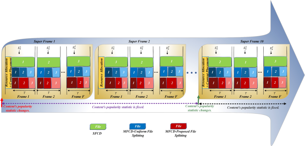
The message passing algorithm (MPA) can be used to detect multiplexed signals on the same subcarriers [32]. In our resource allocation framework, we consider two tasks: content caching and delivery resource allocations. The content caching task deals with determining which content should be cached in which storage. However, the delivery task deals with performing resource allocation such that the contents are delivered to the requesting users within serving time. We assume that the time is split into several super frames. We further assume that each super frame is divided into frames of duration seconds. throughout each supper frame, the arriving users requests, which should be served over the next supper frame, are gathered by the network control system. We emphasize that our proposed content caching and resource allocation algorithms are run for each super frame. Throughout the network run time, the network monitors the file requests and estimate the content distribution (content popularity). At the beginning of each super frame, if a change in the statistics of the contents popularity is detected, joint content caching and radio resource allocation is performed, and otherwise, only radio resource allocation is performed. Note that the proposed resource allocation problem is solved at the beginning of each supper frame, and hence, the information about the CSIs and energy harvesting profile over all frames of the considered supper frame are required and should be known in advanced. With such assumption, we rely on the off-line approach which is common in the context of energy harvesting22 2 In the context of energy harvesting, there is another approach which is called on-line approach. This approach assumes that the information is available only causally and use the Markov decision process method for resource allocation over frames [33]. Although the availability of noncausal information is no practical, the off-line approach would provide a benchmark for energy harvesting networks. We leave the on-line approach as a future research direction [34, 33]. The proposed transmission structure is shown in Fig. 2.
Let denote the codebook assignment at BS at frame where is an indicator variable that is 1 if codebook is assigned to user at BS at frame and 0 otherwise. Furthermore, let denote the allocated transmit power vector with representing the transmit power for user at BS at frame on codebook . Thus, the total transmit power of BS at frame is . To transmit the codewords to the designated users, the transmit power is finally allocated on the corresponding subcarriers. However, different from OFDMA based networks, the transmit power is allocated on subcarrier according to a given proportion , which is determined by the codebook design ( when and when [12]). Therefore, the signal-to-interference-plus-noise ratio (SINR) of user in BS when using codebook can be expressed as follows:
| (1) |
where and denotes the channel power gain between BS and user on subcarrier at time . is the noise power on subcarrier at user . Each of the subcarriers can be assumed to undergo a block-fading, and hence, the channel coefficients are kept constant within each frame. The achievable rate for the user in BS at frame on codebook is given by
We assume that the eavesdroppers only wiretap the access link33 3 Due to the high computing power at the BSs, stronger cryptography is used for the links between core and BSs, hence eavesdropping of these links is hard and difficult. Therefore, we assume that only access link can be wiretapped by eavesdroppers.. Therefore, the SINR of eavesdropper in BS when using codebook can be expressed as:
| (2) |
where and denotes the channel power gain between BS and eavesdropper on subcarrier . is the noise power on subcarrier at eavesdropper . The achievable rate for the eavesdropper in BS at frame is evaluated by The achievable secrecy access rate for non-colluding eavesdroppers and the user in BS at frame on codebook is expressed as [35],
| (3) |
III THE OPTIMIZATION FRAMEWORK
In this section, we provide the design objective and a characterization of the constraints that must be satisfied by content caching, EH, codebook assignment, and power allocations.
III-A System Constraints
III-A1 Content Caching Constraints
Let the finite size of cache memory at the BS is denoted by . If the requested file by user exists in the cache, then the file is sent to the user immediately. This event is referred as a cache hit. However, if file does not exist in the cache, then the request is forwarded to the core network via backhaul, then downloaded file from the core network via backhaul is forwarded to the user. The size of the social media, is assumed to be Log-Normal distributed with parameters and [36]. As the total cached media should not exceed the finite size of cache memory at BS , we have
| (4) |
where is a binary indicator declaring whether social media is cached at BS .
III-A2 Content Delivery
The content delivery consists of two phases: 1) a cache placement phase, and 2) a content delivery phase. In the cache placement phase, the cache content is determined at each BS, and in the content delivery phase, the requested files are delivered to users over wireless channels. In this paper, two new delivery scenarios are considered for content delivery phase. In the first scenario, the user’s requested file with size is sent in a single frame, while in the second scenario the user’s requested file is divided into several parts with sizes , which are sent over several frames. The scenarios are shown in Fig. 2. To ensure that all parts of each file are transmitted to user, the following constraint should be satisfied
| (5) |
III-A3 Access and Backhaul Links Constraints
Let denote whether user needs . The backhaul traffic constraint for BS for the SFCD scenario is written as follows
| (6) | ||||
where the left hand side term of (6) is the backhual traffic for BS and the right hand side term of (6) is backhaul traffic capacity, which must be greater than the backhaul traffic for each BS. The backhaul link is a simple P2M link with OFDMA technology. denotes whether BS uses subcarrier . For the MFCD scenario, in (6) is replaced by as follows
| (7) | ||||
Note that for all requests of social media from BS , if social media is not stored at BS , the requested social media is disseminated to BS from the core network just once. is the rate of backhaul link for BS on subcarrier which is calculated by
| (8) |
When BS receives the data from core network, it transmits the file back on the downlink. Let denotes the received SNR at BS from the core network when the backhaul is used to fetch the files from the core network for BS . can be written as where is the transmit power of each wireless backhaul link connected to BS on subcarrier and denotes the channel power gain between the BS on subcarrier and the core network and is the noise power at the BS on subcarrier . Also the downlink traffic should not exceed the traffic capacity of each downlink. This yields for the first delivery scenario
| (9) |
Note that for the MFCD scenario, in (9) is replaced by as follows:
| (10) |
III-A4 Power Allocation Constraints
To determine the constraints that must be satisfied by any feasible power allocation, let and denote the power allocated to link the BS-the user at time frame on codebook and to link core network-the BS at frame . The elements of and must satisfy the followings:
| (11) |
| (12) |
In a practical network, core network has a power budget, , which bounds the total power allocated by core network on the core network- BS links and subcarriers at frame . This constraint can be written as:
| (13) |
III-A5 EH Constraints
We assume that the BS is connected to a rechargeable battery with capacity , and obtains its power supply through an EH renewable sources such as solar. The renewable sources are used to charge batteries during the day. is defined as the energy remaining in the battery at the start of the frame. Then can be written in recursive form as:
| (14) |
where denotes the amount of energy is harvested during the frame at the BS. The energy arrival takes place as a Poisson arrival process with mean [37, 38]. The unit amount of energy harvested at each arrival at each BS is denoted by , which depends on the EH capabilities of renewable energy source at each BS. Therefore, , where is the number of arrivals within with a mean value of . In designing of optimal transmission policies for EH communication systems, there are main constraints referred to as energy consumption causality constraints, which state that the energy packets which do not arrive yet, cannot be used by a source. These constraints can be expressed as:
| (15) |
If battery capacity is not enough to store the newly arrived energy packet, the energy will be wasted at the beginning of a transmission interval. By considering the following energy overflow constraint on our problem, we avoid this battery overflow by enfrocing the following constraint:
| (16) |
III-A6 Scheduling Constraints
In order to improve the detection performance, we should use the codebooks which have less subcarriers in common. This means that, it must be guaranteed that each subcarrier cannot be reused more than a certain value , i.e., the maximum number of differentiable constellations generated by the codebook-specific constellation function, as follows [16]
| (17) |
III-A7 Worst Case Channel Uncertainty Model
For the channels between the BS and the eavesdropper, only the estimated value is available at the BS. We define the channel error as , and we assume that the channels mismatches are bounded as follows:
| (21) |
where is known constant. Hence the actual channel power gain value lies in the region [39].
III-B The Optimization Problem
We formulate the utility maximization problem with power allocation, codebook assignment, and content caching subject to energy causality and power budget constraints at each BS for the SFCD scenario as:
| (22) | ||||
| s.t. |
where , . Note that for the MFCD scenario, constraint (5) is added to the optimization problem (22). We also replace (6), (9) and (18) by (7), (10) and (19), respectively. It should also be noted that in the second scenario, is itself an optimization variable that must be obtained in the optimization problem. The optimization problem (22) consisting of non-convex objective function and both integer and continuous variables. Hence, it is mixed-integer nonlinear programming (MINLP), non-convex, intractable and NP-hard problem [40].
Lemma 1.
The optimization problem (22) is NP-hard.
Proof.
Please see Appendix A. ∎
It is very difficult to find the global optimal solution within polynomial time. Hence, the available methods to solve convex optimization problem can not be applied directly. To solve this problem, an iterative algorithm based on the well-known and well-proven alternating, Dinkelbach and successive convex approximation methods is proposed where in each iteration, the main problem is decoupled into several sub-problems subject to some optimization variables.
IV PROPOSED SOLUTION
The difficulty of solving the problem (22) arises from the nonconvexity of both the objective function and feasible domain. As far as we know, there is no standard method to solve such a nonconvex optimization problem. In this section, some optimization methods such as alternative optimization, fractional programming, and difference-of-two-concave-functions (DC) programming, are jointly applied to solve the primal problem by transforming it into simple subproblems step by step. To facilitate solving (22), an alternate optimization method is adopted to solve a multi-level hierarchical problem which consists of the several subproblem. The core idea of the alternate optimization is that only one of the optimization parameters is optimized in each step while others are fixed. When each parameter is given, the resulting subproblem can be reformulated as the form of DC problem and solved by DC programming. Moreover, a sequential convex program is finally solved by convex optimization methods at each iteration of the DC programming. In this section, we propose a solution for the SFCD scenario which is suitable for MFCD, too. The transformation process for solving this problem mainly consists of the following steps: I. Transformation of the primal problem: By using the epigraph method, the inner maximization in the objection function in (23) can be simplified and the secondary problem can be naturally derived. II. Alternate optimization over some variables: In this step, the alternate optimization method is adopted to cope with the non-convexity of the resulting parametrized secondary problems which is further rewritten as five sub-problems, namely, access power allocation, access code allocation, backhaul power allocation, backhaul subcarrier allocation, content placement, and channel uncertainty. III. DC programming for the nonconvex constraint elimination: In this step, we reformulate the nonconvex constraint (23c) as a canonical DC programming which can be settled by iteratively solving a series of sequential convex constraints. Finally, these convex constraints can be solved by convex programming. IV. Fractional programming: Applying fractional programming, the parameterized secondary subproblem is solved with a given parameter in each iteration.
IV-A Transformation of the primal problem
IV-B Alternate optimization over optimization variables
Due to the combined non-convexity of both objective function and the constraint with respect to optimization parameters, the optimization problem (22) is difficult to solve. According to alternate optimization method, we can always optimize a function by first optimizing over some of the variables, and then optimizing over the remaining ones. For convenience, the feasible domain of (22) is denoted by as . For fixed , -section of the feasible domain of , i.e., , is defined as . Likewise, for fixed , -section of the feasible domain of , i.e., , is defined as . Similarly, for fixed , -section of the feasible domain of , i.e., , is defined as . In the same way, for fixed , -section of the feasible domain of , i.e., , is defined as . Correspondingly, for fixed , -section of the feasible domain of , i.e., , is defined as . Finally, the alternate optimization is used to solve the following hierarchical five-level optimization subproblem:
| (27) |
In conclusion, the subproblems can be solved sequentially at each iteration of alternate optimization. In the first optimization subproblem, we find for a given , and :
| (28) |
where is the iteration number of alternate optimization algorithm. By defining the solution of (28) as , the second level subproblem is solved to find with a given , and :
| (29) |
Similarly, by defining the solution of (29) as , the third level subproblem is solved to find and with a given , and :
| (30) |
Correspondingly, by defining the solution of (30) as and , the fifth level subproblem is solved to find with a given , and :
| (31) |
Finally, by defining the solution of (31) as , the fifth level subproblem is solved to find with a given :
| (32) |
Let denote the obtained solution at the -th iteration, which should be used for the -th iteration. With a convergence threshold , the stop condition of alternate optimization algorithm is then given by
| (33) | ||||
We can also present a maximum allowed number for . Alternate optimization algorithm is illustrated in Table. I. Furthermore, the following Theorem. 1 can verify the convergence of the alternate optimization algorithm.
Theorem 1.
Proof.
Please see Appendix B. ∎
| Algorithm 1: Alternate Optimization Algorithm |
| Step1: Select a starting point , and Set iteration number ; |
| Step2: Compute ; |
| Repeat |
| Step3: For fixed , solve (34) to obtained the (Linear programming); |
| Step4: For the obtained , and fixed , solve (29) to find (Linear programming); |
| Step5: For the obtained , , and fixed , solve (30) to find and (Convex programming); |
| Step6: For the obtained , , and , and fixed , solve (31) to find (DC programming); |
| Step7: For the obtained , , , and , solve (32) to find and (DC programming); |
| Step8:Compute ; |
| Step9: ; |
| Step10: If or goto Step12, else goto Step3; |
| End |
| Step11: Return . |
IV-B1 Channel Uncertainty Problem
For minimizing the worst-case problem over in (28), we solve the following problem for each , , , , and :
| (34) |
We can rewrite (34) as follows:
| (35a) | ||||
| s.t. | (35b) | |||
| (35c) | ||||
where is a vector of the same dimension as with all zero enry expect for , and is a vector of the same dimension as with , and for all other entries. This problem has a linear fractional objective function, for which, Charnes-Cooper transformation can be used to reformulate it into the following linear programming optimization problem [42]:
| (36a) | ||||
| s.t. | (36b) | |||
| (36c) | ||||
| (36d) | ||||
where , and . Problem (36) can now be efficiently solved using interior-point based methods by some off-the-shelf convex optimization toolboxes, e.g., CVX.
IV-B2 Content Placement
IV-B3 Backhaul Power and Subcarrier Allocation
The optimization problem is still a mixed-integer non-convex programming with respect to and , which is difficult to tackle. To make this problem tractable, we first relax each to a continuous interval, i.e., [0,1]. Further, new variables is defined to replace . Then, we can transform the nonconvex optimization problem into the convex one. This problem can be easily solved by available standard optimization softwares such as CVX with the internal solver MOSEK [1]. Note that this relaxation is called time sharing which shows the time percentage that each subcarrier should be used [44].
IV-B4 Access Power and Codebook Allocation
The optimization problem is still non-convex with respect to p and s. The difficulty of solution comes from the non-convexity of both objective function and secrecy rate constraint. There is no standard approach to solve such a non-convex problem. Therefore, we exploit DC and fractional programming in the next sections to transform it into a tractable problem. In the following, we develop a solution for power allocation optimization problem and we remark that this solution can be developed for code assignment in the same way.
IV-C Difference-of-Two-Concave-Functions (D.C.) Approximation
Due to the non-convexity of (26c), the optimization problem (26) is still difficult to solve. The standard D.C. optimization problem can be written as where and are two convex components with convex feasible domain. This problem can be solved iteratively by solving a sequential convex program as follows:
| (37) |
at each iteration, where is the optimal solution of the iteration used for the iteration and is the gradient of evaluated at . By the sequential convex approximation, DC subproblems are equivalently reformulated as:
| (38a) | ||||
| s.t. | ||||
| (38b) | ||||
where
| (39) | ||||
| (40) |
We first express in a D.C. form as:
| (41) |
Based on (41), the gradient with respect to is given by
| (42) | ||||
Theorem 2.
The sequence derived from the D.C. programming algorithm is monotonically decreasing. ∎
Proof.
Please see Appendix C. ∎
IV-D Fractional Programming
The objective function in (26) is non-convex. The form of (26) can be classified into the nonlinear fractional programming [45]. Therefore, after replacing nonconvex constraints by convex constraints using the D.C. method in the previous section, the Dinkelbach’s algorithm use to solve convex fractional programming. We define the maximum objective functions of the considered system as:
| (43) |
We are now ready to introduce the following theorem for .
Theorem 3.
The maximum value of is achieved if and only if
| (44) | ||||
For and , where
| (45) |
is defined as a parametric program with parameter . ∎
By the Dinkelbach’s method [23] with a initial value of , (45) can be solved iteratively by solving the following problem:
| (46) |
with a given at the iteration, where is the iteration index. can be explained as the secure EE obtained at the previous iteration. In (46), the maximization problem is equivalent to
| (47) |
Let and denote the solution of (48) for a given . After each iteration, should be updated by
| (48) |
The iteration process will be stopped when (44) is satisfied. In practice, we define the terminated condition of the iterative process as:
| (49) | ||||
with a small convergence tolerance . The algorithm of fractional programming is clarified in Algorithm 2, where is the maximum allowed number of iterations considering the computational time. We use the fractional programming Dinkelbach’s algorithm for the convexified problem (38).
Theorem 4.
If problems (50) are solvable, the sequence obtained by Algorithm 1 has the following properties: 1) ; 2) . ∎
Proof.
Please refer to [45]. ∎
Based on the fractional programming, subproblems (50) are associated with a parametric program problem stated as follows:
| (50a) | ||||
| s.t. | ||||
| (50b) | ||||
We propose an iterative algorithm (known as the Dinkelbach method [45]) for solving (50) with an equivalent objective function. The proposed algorithm to obtain power allocation policy p is summarized in Table. II. The convergence to the appropriate energy efficiency is guaranteed. Note that similar algorithm can be used to obtain code allocation policy s.
| Algorithm 3: Fractional Programming Algorithm |
| Step1: Initialize the maximum number of iterations and the maximum tolerance ; |
| Step2: Choose an initial value and set iteration index ; |
| Repeat |
| Step3: Solve problem (50) for a given and obtain power allocation policy (Convex programming); |
| Step5: Update by (48) to obtain ; |
| Step6:; |
| Step7: If or goto Step7, else goto Step3; |
| Step8: Return , . |
| End |
To solve the primary optimization problem, the main optimization problem is decomposed into several subproblems, with each subproblem being in a hierarchical order of the main problem. Depending on different methods to solve each subproblem, the computational complexity of the proposed algorithm is analyzed in Section V.
V Analysis of Computational Complexity of Proposed Algorithm
To solve the primary optimization problem, the main optimization problem is decomposed into several subproblems, with each subproblem being in a hierarchical order of the main problem. The fast gradient algorithm can be used to solve the inner convex subproblems [47]. Then, the convergence of fast gradient algorithm can be written as follows [47]:
| (51) |
where is convergence tolerance. and are defined as the Lipschitz constants by which the Lipschitz conditions are satisfied with the gradients in subproblem (29) and (30), respectively. Moreover, and denote the convexity parameters to satisfy strong convexity of and , respectively. In other words, the fast gradient method is used to solve optimization problem (29) and (30) in and iterations, respectively. The iteration numbers , and are corresponding to the convergence tolerance , and related to subalgorithms. Then, the overall computational complexity associated with the proposed algorithm is dominated by , where and are the iteration numbers of DC programming algorithm. The computational complexity of the proposed solution of the content placement problem is equal to [48] where is the expected iteration numbers. The computational complexity of the our proposed MFCD problem is equal to [48] where is the expected iteration numbers. The computational complexity of the proposed backhaul power and subcarrier allocation problems are equal to and where , , and are the maximum error tolerance and expected iteration numbers, respectively.
By the proposed algorithm, the main problem, which is NP-hard, can be solved in polynomial time. Therefore, the complexity of the proposed algorithm compared to the original problem is far less and manageable. To manage the complexity, Graphics Processing Unit (GPU) can be utilized. By exploiting GPU instead of central processing unit (CPU), new processing methods to accelerate the processing time can be used. In [49], a new framework to accelerate the iterative-based resource allocation by using ASM and SCA has been devised. By using GPU-based resource allocation, the processing time speed-up of about 1500 times compared to CPU-based methods can be achieved. Due to the space limitation, we omit the study of GPU-based version of the proposed algorithms and leave it as future work.
VI Simulation Results
For simulations, we consider a multi-cell downlink SCMA system where users are randomly distributed in an area of circle with the radius of 1 km for each BS as the center. The number of users in circle area of BS is set to , and the total number of subcarriers and codebooks are set to 8 and 28, respectively. The bandwidth of each subcarrier is 180 kHz [50]. The channels between the MBS and its users and SBS and its users are generated with a normalized Rayleigh fading component and a distance-dependent path loss in urban and suburban areas, modeled as and , respectively [50], where is the distance from user to BS in kilometers and is 8 dB log-normal shadowing. We set the frame duration to s [51, 52]. The noise power, is set to dBm. We set and for SCMA [53]. We set the amount of harvested energy per arrival to J, and users request contents by normal random generator. In the most popular caching case, the most popular contents is cached at each BS until its storage is full. In this case, the content popularity is modeled as the Zipf distribution with Zipf parameter equals to 0.8. Simulation results are obtained by averaging over 1000 simulation runs.
VI-A Effect of Maximum Allowable Backhaul Transmission Power
In this part, we obtain the backhaul rate for different values of backhaul transmission power with different values of . The simulation results are compared for different caching scenarios such as no caching, random caching, most popular caching and the proposed caching methods. In no caching case, no contents are stored by any BS. Hence, all the requested contents are served by the core network over the backhaul links [54, 55, 56]. In the random caching strategy, the contents are randomly cached by BSs until storage of BSs is full. Content popularity does not matter in this strategy. In the most popular caching strategy, each BS caches the most popular contents until its storage is full [55, 54]. The results are reported in Fig. 3. As can be seen, for a fixed transmit power, when is increased, the resulting backhaul rate increases. As can be seen from this figure, utilizing the caching strategies can reduce backhaul traffic compared to the no caching scheme. Our proposed caching strategy has nearly 43%, 23.4% and 18.5% performance gain in terms of backhaul rate reduction compared to the no caching scheme for different values of 1, 2, and 3, respectively. It is also notable that the most popular caching strategy causes more reduction in the backhaul traffic, compared to the random caching scheme. However, when all the caching placement are done jointly with the allocation of other network resources, the network performance improves dramatically. This improvement is due to the fact that content placement is done according to network conditions and resources. Besides, as shown in Fig. 3, our caching scheme reduces the total backhaul rate close to almost 11% compared to the most popular caching strategy.
VI-B Effect of Energy Harvesting
Fig. 3 shows the EE as a function of harvested energy per arrival for the SFCD scenario. We compare different EH strategy in terms of EE. In general, by increasing the EH value, the EE is also increased. For larger number of users, the EE is increased. In other words, for the small number of users, there is sufficient power resources, therefore by increasing users, the EE is also increased as shown in Fig. 3. However, for too more users, the power resource will be exhausted and thus some users can not access to network. Even so, due to multiuser diversity, the EE will still increase. For limited battery, due to overflow conditions (16), the stored energy must be used such that there is enough capacity in the battery for newly arrived energy. In this regard, increasing the value of will increase the energy efficiency at first, but with further increasing , the energy efficiency decreases. This is because, from the energy efficiency point of view, the energy consumption would be limited to the amount which maximizes the bit-per-joule quantity. However, for unlimited battery, with increasing , the energy efficiency increases at first, and by further increasing , the energy efficiency becomes constant since no more energy would be consumed as all the arriving energy could be stored in the battery.
VI-C Effect of File Spliting
Fig. 4 shows EE as a function of the harvested energy per arrival, for the SFCD and MFCD scenarios As can be seen from Fig. 4, the MFCD scheme outperforms the SFCD scenario. In the EE communication networks, due to random energy arrivals, there may be not enough energy to transmit file that has big size in the SFCD scheme. In contrast, in the MFCD schemes, file is splitted into the several small size files which can be transmitted in the suitable frames to increase EE. In the uniform file splitting, the file is uniformly splitted into several smaller files with the same size. This scheme has better performance than the SFCD scheme, However, we can improve the network performance by using the our proposed method. In the our proposed MFCD scheme, the best size of each splitted file is obtained to enhance the network performance. This figure also shows that by reducing the size of file, the distance between the graphs for the three scenarios decreases. As seen, the MFCD-proposed file splitting and MFCD-uniform file splitting have closed to almost 9.4% and 6% performance gain in terms of EE compared to SFCD scheme, respectively.
VI-D Transmission Inutility
In this section, we investigate the transmission inutility for the SFCD and MFCD schemes. The transmission inutility is defined by multiplying the outage probability in the transmission delay. The outage probability is defined as probability that there is not enough battery to send content files and the transmission delay is defined as number of frames to send files. Fig. 4 demonstrates the transmission inutilities of our proposed schemes for different content file size. As can be seen, by increasing the size of file, the transmission inutility is increased for both schemes. This is due to the fact that there may be not enough harvested energy to send file, and the energy deficiency probability can be increased. Therefore, the outage probability approaches to one in sufficiently big size of files. This deterioration in the MFCD schemes are less than the SFCD scheme. Because in the MFCD schemes, the deficiency probability of energy can be reduced by dividing the content file into several parts and sending each part in different frames. In the proposed splitting scheme, we find the best fractional of content file for each frame which reduces the outage probability more than before. As shown in Fig. 4, for larger content file sizes, the MFCD scheme has a higher efficiency in reducing the outage probability. As can be seen, for the size of content files less than 3 MBits, the SFCD scheme is better, while for the size of large files, the MFCD scheme is better.
VI-E Effect of Channel Uncertainity
Fig. 5 shows the access secrecy rate versus channel uncertainty for the SFCD scenario. We see that at bigger channel uncertainty, the secrecy access rate clearly has low value. This is due to the fact that when the uncertainty increases, for the worst case scenario, we must guarantee the security for the worst (biggest) channel value of eavesdroppers which leads to low values of secrecy rate. As can be seen, as the number of eavesdroppers increases, the secrecy access rate decreases due to the multiuser diversity gain for eavesdroppers.
VI-F Comparison Between Joint backhaul and access optimization and Disjoint Optimization Problem Solution
Fig. 5 illustrates the comparison between joint optimization and disjoint optimization problem solutions versus different backhaul transmission power for the SFCD scenario. In solving the main problem disjointly, one must solve two optimization problems, one for the access part and the other for the backhaul part. Here, we first solve the backhaul problem since in most cases the backhaul capacity is the limiting factor. For the backhaul problem, the objective is maximization of the backhaul rate, and the constraint is the total transmit power of the backhaul. Solving this problem, the supported transmission rate of the backhaul is obtained which will be used in the access problem. The access problem is similar to the problem (22). The differences between the access problem and problem (22) are that the optimization variables of the backhaul and the constraints relating to the backhaul are removed, and one additional constraint, which states the the access secrecy rate should be above the backhaul transmission rate (obtained in the backhaul problem), is included in the access problem. It can be noticed that the joint backhaul and access optimization approach has better solution than the disjoint backhaul and access optimization approach. This is mainly because that in the joint scenario, the feasibility set of the optimization problem is bigger than the disjoint one. Indeed, in the access problem, we have the constraint which enforces that the access rate should above the backhaul transmission rate (obtained in the backhaul problem) which makes the feasibility set of the disjoint problems smaller than that of the joint one. From Fig. 5, it can be observed that there exists nearly 51.3% and 50% performance gap between joint and disjoint approachs in terms of backhaul and access rates, respectively.
VI-G Effect of super frame size
Fig. 6 shows the variation of the EE with the number of frames, for the SFCD scenario. It is seen that by increasing super frame size, the value of EE increases. In other words, by increasing super frame size, the transmitter can transmit data stream over different frames, then the secrecy access rate and EE will increase. For limited battery storage, with increasing super frame size, at first the EE increases. However, with further increasing super frame size, due to energy overflow constraints, (16), which enforce the transmitters to spend energy, the energy efficiency decreases. Note that, as the value of becomes larger, this decrease in EE happens in lower super frame sizes. For unlimited battery storage, since the overflow constrains, (16), are absent, all the harvested energy is stored in the battery. In this case, increasing super frame size will increase the diversity gain, and hence, the energy efficiency increases.
VI-H The Convergence of the Proposed Algorithm
In this part, we investigate the performance of the proposed resource allocation algorithm. In Fig. 6, we show EE after each iteration at the proposed alternate optimization algorithm. As can be seen, the convergence of the proposed algorithm can averagely be achieved within 700 iterations.
VII Conclusion
In this paper, we provided a unified framework for radio resources allocation and content placement considering the physical layer security and the channel uncertainty to provide higher energy efficiency. To do so, we considered downlink SCMA scenarios, and we aimed at maximizing the worst case energy efficiency subject to system constraints which determines the radio resources allocation and content placement parameter. Moreover, we proposed two novel content delivery scenarios: 1) single frame content delivery, and 2) multiple frames content delivery. In the first scenario, the requested content by each user is served over one frame. However, in the second scenario, the requested content by each user can be delivered over several frames. Since the optimization problems are noncovex and NP-hard, we provided an iterative method converging to a local solution. Finally, we showed the resulting secrecy access rate, backhaul rate, and energy efficiency for different values of maximum backhaul transmit power as well as different number of users and various content size. In addition, we compared the performance of the proposed caching scheme with the existing traditional caching schemes. Based on simulation results, via our proposed caching scheme, the performance is approximately improved by 14% and 21% compared to the most popular and random caching schemes, respectively. Moreover, it can be seen that the MFCD scheme can approximately enhance the system performance by 5.2% and 11.1% for small and large files, respectively.
Appendix A Proof of Lemma 1
We jointly find the optimization variables , and such that the EE of proposed system is maximized. Hence, (22) is MINLP and non-convex. We assume that the optimization variables , and are constant. In access link, we also assume that one subcarrier is exclusively assigned to at most users within the cell. We consider the downlink of an SCMA-based access link consisting of subcarriers, users and . By assuming that the special user’s channel gain on all subcarriers is the largest among all users, the optimal power assigned to user is equal to , where is the transmit power assigned to user at BS at frame on codebook . Then, the challenge is how to allocate the remaining power resource to users over all subcarriers. Thus, no subcarrier can be assigned to more than one user. Therefore, a special case of power and codebook optimization problem with is equivalent to the NP-hard problem considered in [57], and the result follows. Finally, it can be concluded that the main problem (22) is also NP-hard.
Appendix B Proof of Theorem 1
In accordance to the foregoing discussions, for (28) with a given , is its optimal solution, while is only its feasible solution. We get that
| (52) | ||||
Likewise, for (29) with a given , is its optimal solution, while is only its feasible solution. It follows that
| (53) | ||||
For relations (30), (31), and (32), this trend is similar. It is naturally concluded that
| (54) | ||||
Appendix C Proof of Theorem 2
Because of the convexity of , it follows that
| (55) | ||||
for and in the feasible domain. We can deduce that
| (56) | ||||
Obviously, the current value is smaller than the previous value while the current solution is better than the previous solution . As a result, the theorem is proved.
References
- [1] N. Mokari, F. Alavi, S. Parsaeefard, and T. Le-Ngoc, “Limited-feedback resource allocation in heterogeneous cellular networks,” IEEE Transactions on Vehicular Technology, vol. 65, no. 4, pp. 2509–2521, May 2016.
- [2] S. Woo, E. Jeong, S. Park, J. Lee, S. Ihm, and K. Park, “Comparison of caching strategies in modern cellular backhaul networks,” in Proceedings of the 11th annual international conference on Mobile systems, applications, and services, New York, NY, USA, June 2013, pp. 319–332.
- [3] E. Bastug, M. Bennis, and M. Debbah, “Living on the edge: The role of proactive caching in 5G wireless networks,” IEEE Communications Magazine, vol. 52, no. 8, pp. 82–89, August 2014.
- [4] S. Rezvani, N. Mokari, M. R. Javan, and E. A. Jorswieck, “Fairness and transmission-aware caching and delivery policies in OFDMA-based HetNets,” arXiv preprint arXiv:1711.02776, 2017.
- [5] H. Ahlehagh and S. Dey, “Video-aware scheduling and caching in the radio access network,” IEEE/ACM Transactions on Networking (TON), vol. 22, no. 5, pp. 1444–1462, October 2014.
- [6] K. Shanmugam, N. Golrezaei, A. G. Dimakis, A. F. Molisch, and G. Caire, “Femto caching: Wireless content delivery through distributed caching helpers,” IEEE Transactions on Information Theory, vol. 59, no. 12, pp. 8402–8413, September 2013.
- [7] N. Golrezaei, A. F. Molisch, A. G. Dimakis, and G. Caire, “Femtocaching and device-to-device collaboration: A new architecture for wireless video distribution,” IEEE Communications Magazine, vol. 51, no. 4, pp. 142–149, April 2013.
- [8] M. Gregori, J. Gómez-Vilardebò, J. Matamoros, and D. Gündüz, “Joint transmission and caching policy design for energy minimization in the wireless backhaul link,” in Proceedings of IEEE International Symposium on Information Theory (ISIT), Hong Kong, China, June 2015, pp. 1004–1008.
- [9] S. Zhang, N. Zhang, P. Yang, and X. Shen, “Cost-effective cache deployment in mobile heterogeneous networks,” IEEE Transactions on Vehicular Technology, vol. 66, no. 12, pp. 11 264–11 276, July 2017.
- [10] E. M. Yeatman, “Advances in power sources for wireless sensor nodes,” in Proceedings of Intl Workshop on Wearable and Implantable Body Sensor Networks, London, United Kingdom, July 2004, pp. 20–21.
- [11] J. A. Paradiso and T. Starner, “Energy scavenging for mobile and wireless electronics,” IEEE Pervasive Computing, vol. 12, no. 4, pp. 18–27, January 2005.
- [12] N. Hosein and B. Hadi, “Sparse code multiple access,” in Proceedings of IEEE 24th Annual International Symposium on Personal, Indoor, and Mobile Radio Communications (PIMRC), London, UK, September 2013, pp. 332–336.
- [13] K. Au, a. H. N. L. Zhang, A. B. E. Yi, U. Vilaipornsawai, J. Ma, and P. Zhu, “Uplink contention based SCMA for 5G radio access,” in Proceedings of IEEE GLOBECOM, Texas, USA, December 2014, pp. 900–905.
- [14] M. Moltafet, N. Mokari, M. R. Javan, and P. Azmi, “Comparison study between NOMA and SCMA,” IEEE Transactions on Vehicular Technology, October 2017.
- [15] Z. Li, W. Chen, F. Wei, F. Wang, X. Xu, and Y. Chen, “Joint codebook assignment and power allocation for SCMA based on capacity with gaussian input,” in Proceedings of IEEE/CIC International Conference on Communications in China (ICCC), Chengdu, China, July 2016, pp. 1–6.
- [16] Y. Li, M. Sheng, Z. Sun, Y. Sun, L. Liu, D. Zhai, and J. Li, “Cost-efficient codebook assignment and power allocation for energy efficiency maximization in SCMA networks,” in Proceedings of IEEE 84th Vehicular Technology Conference (VTC-Fall), Montreal, QC, Canada, March 2016, pp. 1–5.
- [17] N. Ahmed, M. A. Khojastepour, A. Sabharwal, and B. Aazhang, “Outage minimization with limited feedback for the fading relay channel,” IEEE Transactions on Communications, vol. 54, no. 4, pp. 659–669, April 2006.
- [18] M. R. Javan, N. Mokari, F. Alavi, and A. Rahmati, “Resource allocation in decode-and-forward cooperative communication networks with limited rate feedback channel,” IEEE Transactions on Vehicular Technology, vol. 66, no. 1, pp. 256–267, April 2017.
- [19] I. Csiszár and P. Narayan, “Secrecy generation for multiaccess channel models,” IEEE Transactions on Information Theory, vol. 59, no. 1, pp. 17–31, September 2013.
- [20] A. D. Wyner, “The wire-tap channel,” Bell Labs Technical Journal, vol. 54, no. 8, pp. 1355–1387, 1975.
- [21] F. Alavi, N. M. YAMCHI, M. R. Javan, and K. Cumanan, “Limited feedback scheme for device to device communications in 5G cellular networks with reliability and cellular secrecy outage constraints,” IEEE Transactions on Vehicular Technology, April 2017.
- [22] M. R. Abedi, N. Mokari, M. R. Javan, and H. Yanikomeroglu, “Limited rate feedback scheme for resource allocation in secure relay-assisted OFDMA networks,” IEEE Transactions on Wireless Communications, vol. 15, no. 4, pp. 2604–2618, September 2016.
- [23] L. Wang, K.-K. Wong, S. Jin, G. Zheng, and R. W. Heath Jr, “A new look at physical layer security, caching, and wireless energy harvesting for heterogeneous ultra-dense networks,” arXiv preprint arXiv:1705.09647, May 2017.
- [24] A. Sharma, R. K. Ganti, and J. K. Milleth, “Joint backhaul-access analysis of full duplex self-backhauling heterogeneous networks,” IEEE Transactions on Wireless Communications, vol. 16, no. 3, pp. 1727–1740, January 2017.
- [25] O. Dhifallah, H. Dahrouj, T. Y. Al-Naffouri, and M.-S. Alouini, “Joint hybrid backhaul and access links design in cloud-radio access networks,” in Proceedings of IEEE 82nd Vehicular Technology Conference (VTC Fall), Boston, MA, USA, 2015, pp. 1–5.
- [26] C. Hua, Y. Luo, and H. Liu, “Wireless backhaul resource allocation and user-centric clustering in ultra-dense wireless networks,” IET Communications, vol. 10, no. 15, pp. 1858–1864, October 2016.
- [27] M. Shariat, E. Pateromichelakis, A. ul Quddus, and R. Tafazolli, “Joint TDD backhaul and access optimization in dense small-cell networks,” IEEE Transactions on Vehicular Technology, vol. 64, no. 11, pp. 5288–5299, December 2015.
- [28] H. Zhuang, J. Chen, and D. O. Wu, “Joint access and backhaul resource management for ultra-dense networks,” in Proceedings of IEEE International Conference on Communications (ICC), Paris, France, December 2017, pp. 1–6.
- [29] M. Mirahsan, H. Farmanbar, and H. Yanikomeroglu, “Joint backhaul and access optimization for service-segment-based vn admission control,” in Proceedings of IEEE International Conference on Communications (ICC), Paris, France, December 2017, pp. 1–6.
- [30] Y. Niu, C. Gao, Y. Li, L. Su, D. Jin, and A. V. Vasilakos, “Exploiting device-to-device communications in joint scheduling of access and backhaul for mmwave small cells,” IEEE Journal on Selected Areas in Communications, vol. 33, no. 10, pp. 2052–2069, May 2015.
- [31] “Spectrum and technology issues for microwave backhaul in europe,” Innovation Observatory Ltd, Silvaco Technology Centre, Compass Point Business Park, St Ives, Cambs., PE27 5JL, UK, Tech. Rep., November 2010.
- [32] R. Hoshyar, F. Wathan, and R. Tafazolli, “Novel low-density signature for synchronous CDMA systems over AWGN channel,” IEEE Transactions on Signal Processing, vol. 56, no. 4, pp. 1616–1626, April 2008.
- [33] A. Minasian, S. ShahbazPanahi, and R. S. Adve, “Energy harvesting cooperative communication systems,” IEEE Transactions on Wireless Communications, vol. 13, no. 11, pp. 6118–6131, May 2014.
- [34] Y. Luo, J. Zhang, and K. B. Letaief, “Optimal scheduling and power allocation for two-hop energy harvesting communication systems,” IEEE Transactions on Wireless Communications, vol. 12, no. 9, pp. 4729–4741, August 2013.
- [35] P. C. Pinto, J. Barros, and M. Z. Win, “Secure communication in stochastic wireless networks?part I: Connectivity,” IEEE Transactions on Information Forensics and Security, vol. 7, no. 1, pp. 125–138, 2012.
- [36] P. Sobkowicz, M. Thelwall, K. Buckley, G. Paltoglou, and A. Sobkowicz, “Lognormal distributions of user post lengths in internet discussions-a consequence of the weber-fechner law?” EPJ Data Science, vol. 2, no. 1, p. 2, August 2013.
- [37] O. Ozel, K. Tutuncuoglu, J. Yang, S. Ulukus, and A. Yener, “Transmission with energy harvesting nodes in fading wireless channels: Optimal policies,” IEEE Journal on Selected Areas in Communications, vol. 29, no. 8, pp. 1732–1743, August 2011.
- [38] H. S. Dhillon, Y. Li, P. Nuggehalli, Z. Pi, and J. G. Andrews, “Fundamentals of heterogeneous cellular networks with energy harvesting,” IEEE Transactions on Wireless Communications, vol. 13, no. 5, pp. 2782–2797, July 2014.
- [39] Y. Liang, G. Kramer, H. V. Poor, and S. Shamai, “Compound wiretap channels,” EURASIP Journal on Wireless Communications and Networking, vol. 2009, p. 5, 2009.
- [40] K. G. Murty and S. N. Kabadi, “Some NP-complete problems in quadratic and nonlinear programming,” Mathematical programming, vol. 39, no. 2, pp. 117–129, 1987.
- [41] N. Van Thoai, “Solution methods for general quadratic programming problem with continuous and binary variables: Overview,” in Advanced Computational Methods for Knowledge Engineering. Springer, 2013, pp. 3–17.
- [42] S. Parsaeefard, A. R. Sharafat, and N. Mokari, Robust resource allocation in future wireless networks. Springer, 2017.
- [43] G. Michael, B. Stephen, and Y. Ye, “Matlab software for disciplined convex programming, version 2.0 beta,” Recent Advances in Learning and Control, pp. 95–110, 2012.
- [44] M. Tao, Y.-C. Liang, and F. Zhang, “Resource allocation for delay differentiated traffic in multiuser OFDM systems,” IEEE Transactions on Wireless Communications, vol. 7, no. 6, pp. 2190–2201, 2008.
- [45] W. Dinkelbach, “On nonlinear fractional programming,” Management Science, vol. 13, no. 4, pp. 492–498, March 1967.
- [46] S. Schaible, “Fractional programming. II, On Dinkelbachs algorithm,” Management Science, vol. 22, no. 8, pp. 868–873, April 1976.
- [47] S. Richter, C. N. Jones, and M. Morari, “Computational complexity certification for real-time MPC with input constraints based on the fast gradient method,” IEEE Transactions on Automatic Control, vol. 57, no. 6, pp. 1391–1403, 2012.
- [48] A. Ben-Tal and A. Nemirovski, Lectures on modern convex optimization: analysis, algorithms, and engineering applications. SIAM, 2001.
- [49] A. Mokdad, P. Azmi, N. Mokari, M. Moltafet, and M. Ghaffari-Miab, “Cross-layer energy efficient resource allocation in PD-NOMA based H-CRANs: Implementation via GPU,” Availible on arXiv, 2018.
- [50] T. ETSI, “136 931 v9. 0.0,LTE; evolved universal terrestrial radio access (E-UTRA); radio frequency (RF) requirements for LTE pico node B,” 3GPP TR 36.931 version 9.0. 0 Release 9), 2011. Online at: http://www. etsi. org/deliver/etsi_ts/136100_136199/13610 4/09.04. 00_60/ts_136104v090400p. pdf, Tech. Rep., 2011.
- [51] P. Castiglione and G. Matz, “Energy-neutral source-channel coding with battery and memory size constraints,” IEEE Transactions on Communications, vol. 62, no. 4, pp. 1373–1381, March 2014.
- [52] F. Zhang and V. K. Lau, “Delay-sensitive dynamic resource control for energy harvesting wireless systems with finite energy storage,” IEEE Communications Magazine, vol. 53, no. 8, pp. 106–113, 2015.
- [53] H. Nikopour and H. Baligh, “Sparse code multiple access,” in Proceedings of IEEE 24th International Symposium on Personal Indoor and Mobile Radio Communications (PIMRC), London, UK, November 2013, pp. 332–336.
- [54] S.-H. Park, O. Simeone, and S. S. Shitz, “Joint optimization of cloud and edge processing for fog radio access networks,” IEEE Transactions on Wireless Communications, vol. 15, no. 11, pp. 7621–7632, September 2016.
- [55] R. G. Stephen and R. Zhang, “Green OFDMA resource allocation in cache-enabled CRAN,” in Proceedings of IEEE Online Conference on Green Communications (OnlineGreenComm), Piscataway, NJ, USA, December 2016, pp. 70–75.
- [56] H. Hsu and K.-C. Chen, “A resource allocation perspective on caching to achieve low latency,” IEEE Communications Letters, vol. 20, no. 1, pp. 145–148, November 2016.
- [57] L. Lei, D. Yuan, C. K. Ho, and S. Sun, “Joint optimization of power and channel allocation with non-orthogonal multiple access for 5g cellular systems,” in 2015 IEEE Global Communications Conference (GLOBECOM), 2015, pp. 1–6.