Invertible Autoencoder for domain adaptation
Abstract
The unsupervised image-to-image translation aims at finding a mapping between the source () and target () image domains, where in many applications aligned image pairs are not available at training. This is an ill-posed learning problem since it requires inferring the joint probability distribution from marginals. Joint learning of coupled mappings and is commonly used by the state-of-the-art methods, like CycleGAN (Zhu et al., 2017), to learn this translation by introducing cycle consistency requirement to the learning problem, i.e. and . Cycle consistency enforces the preservation of the mutual information between input and translated images. However, it does not explicitly enforce to be an inverse operation to . We propose a new deep architecture that we call invertible autoencoder (InvAuto) to explicitly enforce this relation. This is done by forcing an encoder to be an inverted version of the decoder, where corresponding layers perform opposite mappings and share parameters. The mappings are constrained to be orthonormal. The resulting architecture leads to the reduction of the number of trainable parameters (up to times). We present image translation results on benchmark data sets and demonstrate state-of-the art performance of our approach. Finally, we test the proposed domain adaptation method on the task of road video conversion. We demonstrate that the videos converted with InvAuto have high quality and show that the NVIDIA neural-network-based end-to-end learning system for autonomous driving, known as PilotNet, trained on real road videos performs well when tested on the converted ones.
1 Introduction
| o X[c] X[c] X[c] X[c] InvAuto | Auto | Cycle | VAE |


Inter-domain translation problem of converting an instance, e.g.: image or video, from one domain to another is applicable to a wide variety of learning tasks, including object detection and recognition, image categorization, sentiment analysis, action recognition, speech recognition, and more. High-quality domain translators ensure that an arbitrary learning model trained on the samples from the source domain, can perform well when tested on the translated samples11 1 Similarly, an arbitrary learning model trained on the translated samples should perform well on the samples from the target domain. Training in this framework is however much more computationally expensive.. The translation problem can be posed in the supervised learning framework, e.g.: (Isola et al., 2017; Wang et al., 2017), where the learner has access to corresponding pairs of instances from both domains, or unsupervised learning framework, e.g.: (Zhu et al., 2017; Liu et al., 2017), where no such paired instances are available. This paper focuses on the latter case, which is more difficult but at the same time more realistic as acquiring the data set of paired images is often impossible in practice.
The unsupervised domain adaptation is typically solved using generative adversarial networks (GAN) framework (Goodfellow et al., 2014), where the generator performs domain translation and is trained to learn the mapping from the source to the target domain and the discriminator is trained to discriminate between original images from the target domain and those provided by the generator. In this setting, the generator usually has the structure of the autoencoder. The two most common state-of-the-art domain adaptation approaches, CycleGAN (Zhu et al., 2017) and UNIT (Liu et al., 2017), are built on this basic approach. CycleGAN addresses the problem of adaptation from domain to domain by training two translation networks, where one realizes the mapping and the other realizes . The cycle consistency loss ensures the correlation between input image and the corresponding translation. In particular, to achieve cycle consistency, CycleGAN trains two autoencoders, where each minimizes its own adversarial loss and they both jointly minimize
| (1) |
Cycle consistency loss is also incorporated into the recent implementations of UNIT. It is implicitly assumed that the model will learn the mappings and in such a way that , however it is not explicitly imposed. Consider a simple example. Assume the first autonecoder is a -layer linear multi-layer perceptron (MLP) where the weight matrix of the first layer (encoder) is denoted as and the weight matrix of the second layer (decoder) is denoted as . Thus, for an input it outputs . The second autoencoder then is a -layer MLP with encoder weight matrix and decoder weight matrix that for an input data point should produce output . To satisfy cycle consistency requirement, the following should hold: and . These two conditions are equivalent to and . This holds for example when and .
In contrast to this approach, we implicitly require . Thus, in the context of the given simple example, we correlate encoders and decoders to satisfy inversion conditions and . We avoid performing prohibitive inversions of large matrices and instead guarantee these conditions to hold through two steps: (i) introducing shared parametrization of encoder and decoder such that ( and is treated similarly) and (ii) appropriate training to achieve orthonormality and , i.e. we train autoencoder to satisfy for arbitrary input and autoencoder to satisfy for arbitrary input . Since the encoder and decoder are coupled as given in (i), such training leads to satisfying inversion conditions. Practical networks contain linear and non-linear transformations. We therefore propose specific architectures, which are invertible.
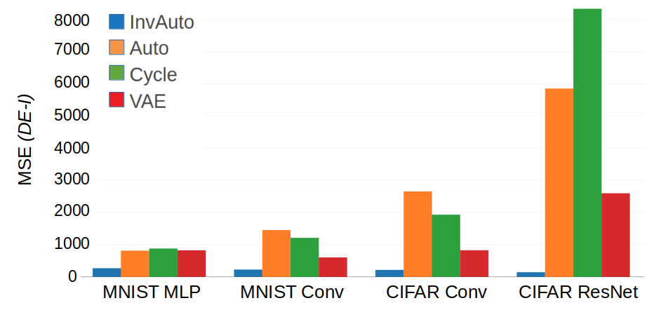
Figure 1 (see also its extended version, Figure 17, in the Supplement) and 2 illustrate the basic idea behind InvAuto. The plots were obtained by training a single autoencoder to reconstruct its input. InvAuto has shared weights satisfying and inverted non-linearities and clearly obtains matrix that is the closest to identity compared to other methods, i.e. vanilla autoencoder (Auto), autoencoder with cycle consistency (Cycle), and variational autoencoder (VAE) (Kingma & Welling, 2014). Note also that at the same time InvAuto requires half of the number of trainable parameters.
2 Related Work
Unsupervised image-to-image translation models were developed to tackle domain adaptation problem with unpaired data sets. A plethora of existing approaches utilize autoencoders trained in the GAN framework, where autoencoder serves as a generator, for this learning problem. This includes approaches based on conditional GAN (Dong et al., 2017; Wang et al., 2017) and methods introducing additional components to the loss function forcing partial cycle consistency (Taigman et al., 2016). Another approach (Liu & Tuzel, 2016) introduces two coupled GANs, where each generator is an autoencoder and the coupling is obtained by sharing a subset of weights between autoencoders as well as between discriminators. This technique was later on extended to utilize variational autoencoders as generators (Liu et al., 2017). The resulting approach is commonly known as UNIT. CycleGAN presents yet another way of addressing the image-to-image translation by specific training scheme that preserves the mutual information between input and translated images (Vincent et al., 2008). Both UNIT and CycleGAN constitute the most popular choices for performing image-to-image translation.
There also exist other learning tasks that can be viewed as instances of image-to-image translation problem. Among them, notable approaches focus on style transfer (Gatys et al., 2016b; Johnson et al., 2016; Ulyanov et al., 2016; Gatys et al., 2016a). They aim at preserving the content of the input image while altering its style to mimic the style of the images from the target domain. This goal is achieved by introducing content and style loss functions that are jointly optimized. Finally, inverse problems, such as super-resolution, also fall into the category of image-to-image translation problems (McCann et al., 2017).
3 Invertible autoencoder
Here we explain the details of the architecture of InvAuto. The architecture needs to be symmetric to allow invertibility, e.g.: the layers should be arranged as , where denote subsequent transformations of the signal that is being propagated through the network ( is the total number of those) and denote their inversions. Thus, the architecture is inverted layer by layer, where any layer of the encoder has its mirror inverted counterpart in the decoder. The autoencoder is trained to reconstruct its input. Below we explain how to invert different types of layers of the deep model.
3.1 Fully-connected layer
Consider transformation of an input signal performed by an arbitrary fully-connected layer of an encoder parametrized with weight matrix . Let denote layer’s input and denote its output. Thus
| (2) |
An inverse operation is then defined as
| (3) |
We parametrize the counterpart layer of the decoder with a transpose of , thus the considered encoder and decoder layers will share parametrization. Therefore, we enforce the counterpart decoder’s layer to perform transformation:
| (4) |
By training the autoencoder to reconstruct its input on its output we will enforce orthonormality and thus equivalence of transformations and , i.e. .
3.2 Convolutional layer
Consider transformation of an input image performed by an arbitrary convolutional layer of an encoder . Let denote layer’s vectorized input image and denote corresponding output. D convolution can be implemented using matrix multiplication involving a Toeplitz matrix (Vasudevan et al., 2017). Toeplitz matrix is obtained from the set of kernels of the D convolutional filters . Thus transformation and its inverse can be explained with the same equations as the ones used before, Equations 2 and 8, however now is a Toeplitz matrix. We will again parametrize the counterpart layer of the decoder with a transpose of a Toeplitz matrix . The transpose of the Toeplitz matrix is in practice obtained by copying weights from the considered convolutional layer to the counterpart decoder’s layer that is implemented as a transposed convolutional layer (also known as a deconvolutional layer). Therefore, as before, we enforce the counterpart decoder’s layer to perform transformation and by appropriate training ensure .
3.3 Activation function
Invertible activation function should be a bijection. In this paper we consider a modified LeakyReLU activation function and use only this non-linearity in the model. Consider transformation of an input signal performed by this non-linearity applied in the encoder . This non-linearity is defined as
| (5) |
An inverse operation is then defined as
| (6) |
The corresponding non-linearity in the decoder will therefore realize the operation of an inverted modified LeakyReLU given in Equation 6. In the experiments we set .
3.4 Residual block


Consider transformation of an input signal performed by a residual block (He et al., 2016) of an encoder . We modify the residual block to remove the internal non-linearity as given in Figure 3a. The residual block is parametrized with weight matrices and . Those are Toeplitz matrices corresponding to the convolutional and transposed convolutional layers of the residual block. Let denote block’s vectorized input and denote its corresponding output. Thus transformation is defined as
| (7) |
An inverse operation is then defined as
| (8) |
We will parametrize the counterpart residual block of the decoder with a transpose of matrix as given in Figure 3b. Therefore we enforce the counterpart decoder’s residual block to perform transformation:
| (9) |
Similarly as before, at training will enforce orthonormality and thus .
3.5 Bias
We consider bias as a separate layer in the network. Then, handling biases is straightforward. In particular, the layer in the encoder that perform bias addition has its counterpart layer in the decoder, where the same bias is subtracted.
| o X[c] X[c] X[c] X[c] InvAuto | Auto | Cycle | VAE |


3.6 Experimental validation of orthonormality
In this section, we validate the concept of InvAuto. The goal of this section is to show that proposed shared parametrization and training enforce orthonormality and that at the same time the orthonormality property is not organically achieved by standard architectures. We compare InvAuto with previously mentioned vanilla autoencoder, autoencoder with cycle consistency, and variational autoencoder. We experimented with various data sets (MNIST and CIFAR-10) and architectures (MLP, convolutional (Conv), and ResNet). All the networks were designed to have down-sampling layers and up-sampling layers. Encoder’s matrix and decoder’s matrix are constructed by multiplying the weight matrices of consecutive layers of encoder and decoder, respectively.
| Data set | InvAuto | Auto | Cycle | VAE |
|---|---|---|---|---|
| and model | ||||
| MNIST | ||||
| MLP | ||||
| MNIST | ||||
| Conv | ||||
| CIFAR | ||||
| Conv | ||||
| CIFAR | ||||
| ResNet |
| Data set | InvAuto | Auto | Cycle | VAE |
|---|---|---|---|---|
| and model | ||||
| MNIST | ||||
| MLP | ||||
| MNIST | ||||
| Conv | ||||
| CIFAR | ||||
| Conv | ||||
| CIFAR | ||||
| ResNet |
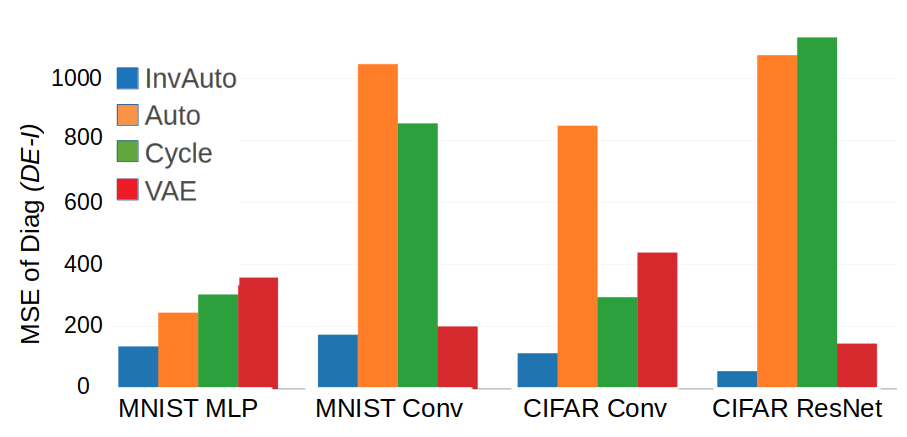
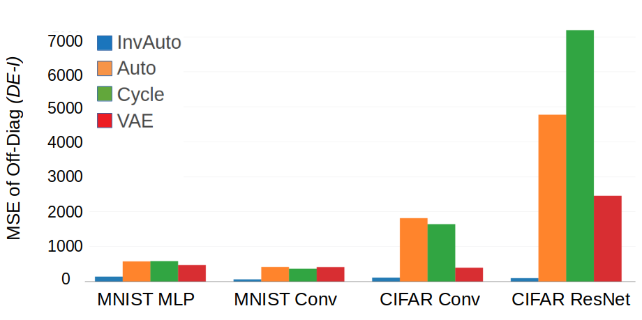
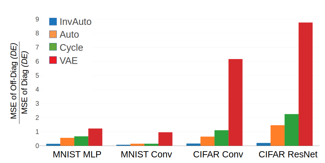
We test orthonormality by reporting the histograms of the cosine similarity of each pair of rows of matrix for all methods (Figure 4) along with their mean and standard deviation (Table 1) as we expect the cosine similarity to be close to for InvAuto. We then show the -norm of the rows of as we expect the rows of InvAuto to have close-to-unit norm (Table 2). InvAuto enforces the encoder, and consequently the decoder, to be orthonormal. Other methods do not explicitly demand that and thus the orthonormality of their encoders is weaker. This observation is further confirmed by Figures 1 and 2 shown before in the Introduction. In the Supplement (Section A), we provide three more figures that complement Figure 2 (recall that the latter reports the MSE of ). They show the MSE of the diagonal (Figure 14) and off-diagonal of (Figure 15) as well as the ratio of the MSE of the off-diagonal and diagonal of (Figure 16) for various methods. The reconstruction loss obtained for all methods is also shown in Section A in the Supplement (Table 5).
Next we describe how InvAuto is applied to the problem of domain adaptation.

4 Invertible autoencoder for domain adaptation
For the purpose of performing domain adaptation we construct the dedicated architecture that is similar to CycleGAN, but we use InvAuto at the feature level of the generators. This InvAuto contains encoder and decoder that themselves have the form of autoencoders. Each of these internal autoencoders is used to do the conversion between the features corresponding to two different domains. And thus, the encoder performs the conversion from the features corresponding to domain into the features corresponding to domain . The decoder , on the other hand, performs the conversion from the features corresponding to domain into the features corresponding to domain . Since and form InvAuto, realizes an inversion of (and vice versa) and shares parameters with . This introduces strong correlations between two generators and reduces the number of trainable parameters, which distinguishes our approach from CycleGAN. The proposed architecture is illustrated in Figure 5. The details of the architecture and training are provided in Section C in the Supplement.
Next we describe the cost function that we use to train our deep model. The first component of the cost function is the adversarial loss (Goodfellow et al., 2014), i.e.
| (10) |
where and denote the distribution of data from and , respectively.
The second component of the loss function is the cycle consistency loss defined as
| (11) |
The objective function that we minimize therefore becomes
| (12) |
where controls the balance between the adversarial loss and cycle consistency loss. The cycle consistency loss enforces the orthonormality property of InvAuto.
5 Experiments
We next demonstrate the experiments on domain adaptation problems. We compare our model against UNIT(Liu et al., 2017) and CycleGAN(Zhu et al., 2017). We used publicly available implementations of both methods available from https://github.com/mingyuliutw/UNIT/ and https://github.com/junyanz/pytorch-CycleGAN-and-pix2pix/.The details of our architecture and the training process are summarized in Section C in the Supplement.
5.1 Experiments with benchmark data sets
We considered the following domain adaptation tasks:
- (i)
Day-to-night and night-to-day image conversion: we used unpaired road pictures recorded during the day and at night obtained from KAIST data set (Hwang et al., 2015).
- (ii)
Day-to-thermal and thermal-to-day image conversion: we used road pictures recorded during the day with a regular camera and a thermal camera obtained from KAIST data set(Hwang et al., 2015).
- (iii)
Maps-to-satellite and satellite-to-maps: we used satellite images and maps obtained from Google Maps (Isola et al., 2017).
The data sets for the last two tasks, i.e. (ii) and (iii), are originally paired, however we randomly permuted them and train the model in an unsupervised fashion. The training and testing images were furthermore resized to resolution.
The visual results of image conversion are presented in Figures 6-11 (Section B in the Supplement contains the same figures in higher resolution). We see that InvAuto visually performs comparably to other state-of-the-art methods.
| o 0.48X[c] X[c] X[c] X[c] Original | CycleGAN | UNIT | InvAuto |

| o 0.48X[c] X[c] X[c] X[c] Original | CycleGAN | UNIT | InvAuto |

| o 0.47X[c] X[c] X[c] X[c] X[c] Original | CycleGAN | UNIT | InvAuto | Reference |

| o 0.47X[c] X[c] X[c] X[c] X[c] Original | CycleGAN | UNIT | InvAuto | Reference |

To evaluate the performance of the methods numerically we use the following approach:
- •
For the tasks (ii) and (iii), we directly calculated the loss between the converted images and the ground truth.
- •
For the task (i), we trained two autoencoders and on both domains, i.e. we trained each of them to reconstruct well the images from its own domain and reconstruct badly the images from the other domain. Then we use these two autoencoders to evaluate the quality of the converted images, where high reconstruction loss of the autoencoder for the images converted to resemble those from its corresponding domain implies low-quality image translation.
Table 3 contains the results of the numerical evaluation and shows that the performance of InvAuto is similar to the state-of-the-art techniques that we compare InvAuto with and is furthermore contained within the performance range established by the CycleGAN (best performer) and UNIT (consistently slightly worst from CycleGAN).
| o 0.47X[c] X[c] X[c] X[c] X[c] Original | CycleGAN | UNIT | InvAuto | Reference |

| o 0.47X[c] X[c] X[c] X[c] X[c] Original | CycleGAN | UNIT | InvAuto | Reference |

| Methods | |||
|---|---|---|---|
| Tasks | CycleGAN | UNIT | InvAuto |
| Night-to-day | |||
| Day-to-nigth | |||
| Thermal-to-day | |||
| Day-to-thermal | |||
| Maps-to-satellite | |||
| Satellite-to-maps | |||
5.2 Experiments with autonomous driving system
To test the quality of the image-to-image translations obtained by InvAuto, we use the NVIDIA evaluation system for autonomous driving described in details in (Bojarski et al., 2016). The system evaluates the performance of an already trained NVIDIA neural-network-based end-to-end learning platform for autonomous driving (PilotNet) on a test video using a simulator for autonomous driving. The system uses the following performance metrics for evaluation: autonomy, position precision, and comfort. We do not describe these metrics as they are described well in the mentioned paper. We only emphasize that these metrics are expressed as a percentage, where corresponds to the best performance. We collected the high-resolution videos of the same road during the day and night from the camera inside the car. Each video had K frames. The pictures were resized to resolution for the conversion and then resized back to the original size of . We used our domain translator as well as CycleGAN to convert the collected day video to a night video (Figure 12) and also the collected night video to a day video (Figure 13). To evaluate our model, we used aforementioned NVIDIA evaluation system, where the converted videos where used as testing sets for this system. We report results in Table 4.
| Video type | Autonomy | Position | Comfort |
|---|---|---|---|
| precision | |||
| Original day | |||
| Original night | |||
| Day-to-night | |||
| InvAuto | |||
| Night-to-day | |||
| InvAuto | |||
| Day-to-night | |||
| CycleGAN | |||
| Night-to-day | |||
| CycleGAN |
The PilotNet model used for testing was trained mostly on day videos, thus it is expected to perform worse on night videos. Therefore the performance for original night video is worse than for the same video converted to a day video in terms of autonomy and position precision. The comfort deteriorates due to the inconsistency of consecutive frames in the converted video, i.e. the videos are converted frame-by-frame and we do not apply any post-processing to ensure smooth transition between frames. The results for InvAuto and CycleGAN are comparable.
6 Conclusion
We proposed a novel architecture that we call invertible autoencoder, which, as opposed to the common deep learning architectures, allows the layers of the model performing opposite operations (like encoder and decoder) to share weights. This is achieved by enforcing orthonormal mappings in the layers of the model. We demonstrate the applicability of the proposed architecture to the problem of domain adaptation and evaluate it on benchmark data sets and autonomous driving task. The performance of the proposed approach matches state-of-the-art methods and requires less trainable parameters.
References
- Bojarski et al. (2016) Bojarski, M., Del Testa, D., Dworakowski, D., Firner, B., Flepp, B., Goyal, P., Jackel, L. D., Monfort, M., Muller, U., Zhang, J., Zhang, X., Zhao, J., and Zieba, K. End to end learning for self-driving cars. CoRR, abs/1604.07316, 2016.
- Dong et al. (2017) Dong, H., Neekhara, P., Wu, C., and Guo, Y. Unsupervised image-to-image translation with generative adversarial networks. CoRR, abs/1701.02676, 2017.
- Gatys et al. (2016a) Gatys, L. A., Bethge, M., Hertzmann, A., and Shechtman, E. Preserving color in neural artistic style transfer. CoRR, abs/1606.05897, 2016a.
- Gatys et al. (2016b) Gatys, L. A., Ecker, A. S., and Bethge, M. Image style transfer using convolutional neural networks. In CVPR, 2016b.
- Goodfellow et al. (2014) Goodfellow, I. J., Pouget-Abadie, J., Mirza, M., Xu, B., Warde-Farley, D., Ozair, S., Courville, A. C., and Bengio, Y. Generative adversarial nets. In NIPS, 2014.
- He et al. (2016) He, K., Zhang, X., Ren, S., and Sun, J. Deep residual learning for image recognition. In CVPR, 2016.
- Hwang et al. (2015) Hwang, S., Park, J., Kim, N., Choi, Y., and Kweon, I. S. Multispectral pedestrian detection: Benchmark dataset and baseline. In CVPR, 2015.
- Isola et al. (2017) Isola, P., Zhu, J.-Y., Zhou, T., and Efros, A. A. Image-to-image translation with conditional adversarial networks. In CVPR, 2017.
- Johnson et al. (2016) Johnson, J., Alahi, A., and Fei-Fei, Li. Perceptual losses for real-time style transfer and super-resolution. In ECCV, 2016.
- Kingma & Ba (2014) Kingma, D. P. and Ba, J. Adam: A method for stochastic optimization. CoRR, abs/1412.6980, 2014.
- Kingma & Welling (2014) Kingma, D. P. and Welling, M. Auto-encoding variational bayes. In ICLR, 2014.
- Liu & Tuzel (2016) Liu, M.-Y. and Tuzel, O. Coupled generative adversarial networks. In NIPS. 2016.
- Liu et al. (2017) Liu, M.-Y., Breuel, T., and Kautz, J. Unsupervised image-to-image translation networks. In NIPS, 2017.
- McCann et al. (2017) McCann, M. T., Jin, K. H., and Unser, M. Convolutional neural networks for inverse problems in imaging: A review. IEEE Signal Process. Mag., 34(6):85–95, 2017.
- Taigman et al. (2016) Taigman, Y., Polyak, A., and Wolf, L. Unsupervised cross-domain image generation. CoRR, abs/1611.02200, 2016.
- Ulyanov et al. (2016) Ulyanov, D., Lebedev, V., Vedaldi, A., and Lempitsky, V. S. Texture networks: Feed-forward synthesis of textures and stylized images. In ICML, 2016.
- Vasudevan et al. (2017) Vasudevan, A., Anderson, A., and Gregg, D. Parallel multi channel convolution using general matrix multiplication. In ASAP, 2017.
- Vincent et al. (2008) Vincent, P., Larochelle, H., Bengio, Y., and Manzagol, P.-A. Extracting and composing robust features with denoising autoencoders. In ICML, 2008.
- Wang et al. (2017) Wang, T.-C., Liu, M.-Y., Zhu, J.-Y., Tao, A., Kautz, J., and Catanzaro, B. High-resolution image synthesis and semantic manipulation with conditional gans. CoRR, abs/1711.11585, 2017.
- Zhu et al. (2017) Zhu, J.-Y., Park, T., Isola, P., and Efros, A. A. Unpaired image-to-image translation using cycle-consistent adversarial networks. In ICCV, 2017.
Invertible Autoencoder for domain adaptation
(Supplementary material)
Appendix A Additional plots and tables for Section 3.6
| Data set | InvAuto | Auto | Cycle | VAE |
|---|---|---|---|---|
| and model | ||||
| MNIST | ||||
| MLP | ||||
| MNIST | ||||
| Conv | ||||
| CIFAR | ||||
| Conv | ||||
| CIFAR | ||||
| ResNet |
| o X[c] X[c] X[c] X[c] InvAuto | Auto | Cycle | VAE |


Appendix B Additional experimental results for Section 5
| o X[c] X[c] X[c] X[c] Original | CycleGAN | UNIT | InvAuto |
| o X[c] X[c] X[c] X[c] Original | CycleGAN | UNIT | InvAuto |
| o X[c] X[c] X[c] X[c] X[c] Original | CycleGAN | UNIT | InvAuto | Reference |
| o X[c] X[c] X[c] X[c] X[c] Original | CycleGAN | UNIT | InvAuto | Reference |
| o X[c] X[c] X[c] X[c] X[c] Original | CycleGAN | UNIT | InvAuto | Reference |
| o X[c] X[c] X[c] X[c] X[c] Original | CycleGAN | UNIT | InvAuto | Reference |
| o X[c] X[c] X[c] Original | CycleGAN | InvAuto |
![[Uncaptioned image]](1802.06869v1/nvidia_data_A.png)
| o X[c] X[c] X[c] Original | CycleGAN | InvAuto |
![[Uncaptioned image]](1802.06869v1/nvidia_data_B.png)
Appendix C Invertible autoencoder for domain adaptation: architecture and training
Generator architecture Our implementation of InvAuto contains invertible residual blocks for both and images, where blocks are used in the encoder and the remaining in the decoder. All layers in the decoder are the inverted versions of encoder’s layers. We furthermore add two down-sampling layers and two up-sampling layers for the model trained on images, and three down-sampling layers and three up-sampling layers for the model trained on images. The details of the generator’s architecture are listed in Table 7 and Table 8. For convenience, we use Conv to denote convolutional layer, ConvNormReLU to denote Convolutional-InstanceNorm-LeakyReLU layer, InvRes to denote invertible residual block, and Tanh to denote hyperbolic tangent activation function. The negative slope of LeakyReLU function is set to . All filters are square and we have the following notations: represents filter size and represents the number of output feature maps. The paddings are added correspondingly.
Discriminator architecture We use similar discriminator architecture as PatchGAN (Isola et al., 2017). It is described in Table 6. We use this architecture for training both on and images.
Criterion and Optimization At training, we set and use loss for the cycle consistency in Equation 12. We use Adam optimizer(Kingma & Ba, 2014) with learning rate = 0.0002, and . We also add penalty with weight .
| Name | Stride | Filter |
|---|---|---|
| ConvNormReLU | 2 2 | K4-F64 |
| ConvNormReLU | 2 2 | K4-F128 |
| ConvNormReLU | 2 2 | K4-F256 |
| ConvNormReLU | 1 1 | K4-F512 |
| Conv | 1 1 | K4-F1 |
| Name | Stride | Filter |
|---|---|---|
| ConvNormReLU | 1 1 | K7-F64 |
| ConvNormReLU | 2 2 | K3-F128 |
| ConvNormReLU | 2 2 | K3-F256 |
| InvRes | 1 1 | K3-F256 |
| InvRes | 1 1 | K3-F256 |
| InvRes | 1 1 | K3-F256 |
| InvRes | 1 1 | K3-F256 |
| InvRes | 1 1 | K3-F256 |
| InvRes | 1 1 | K3-F256 |
| InvRes | 1 1 | K3-F256 |
| InvRes | 1 1 | K3-F256 |
| InvRes | 1 1 | K3-F256 |
| ConvNormReLU | 1/2 1/2 | K3-F128 |
| ConvNormReLU | 1/2 1/2 | K3-F64 |
| Conv | 1 1 | K7-F3 |
| Tanh |
| Name | Stride | Filter |
|---|---|---|
| ConvNormReLU | 1 1 | K7-F64 |
| ConvNormReLU | 2 2 | K3-F128 |
| ConvNormReLU | 2 2 | K3-F256 |
| ConvNormReLU | 2 2 | K3-F512 |
| InvRes | 1 1 | K3-F512 |
| InvRes | 1 1 | K3-F512 |
| InvRes | 1 1 | K3-F512 |
| InvRes | 1 1 | K3-F512 |
| InvRes | 1 1 | K3-F512 |
| InvRes | 1 1 | K3-F512 |
| InvRes | 1 1 | K3-F512 |
| InvRes | 1 1 | K3-F512 |
| InvRes | 1 1 | K3-F512 |
| ConvNormReLU | 1/2 1/2 | K3-F256 |
| ConvNormReLU | 1/2 1/2 | K3-F128 |
| ConvNormReLU | 1/2 1/2 | K3-F64 |
| Conv | 1 1 | K7-F3 |
| Tanh |