Dynamics of decoherence of an entangled pair of qubits locally connected to a one-dimensional disordered spin chain
Abstract
We study the non-equilibrium evolution of concurrence of a Bell pair constituted of two qubits, through the measurement of Loschmidt echo (LE) under the scope of generalized central spin model. The qubits are locally coupled to a one dimensional disordered Ising spin chain. We first show that in equilibrium situation the derivative of LE is able to detect the extent of Griffiths phase that appeared in presence of disordered transverse field only. While in the non-equilibrium situation, the spin chain requires a temporal window to realize the effect of disorder. We show that within this timescale, LE falls off exponentially and this decay is maximally controlled by the initial states and coupling strength. Our detail investigation suggests that there actually exist three types of exponential decay, a Gaussian decay in ultra short time scale followed by two exponential decay in the intermediate time with two different decay exponents. The effect of the disorder starts appearing in the late time power law fall of LE where the power law exponent is strongly dependent on disorder strength and the final state but almost independent of initial states and coupling strength. This feature allows us to indicate the presence of Griffiths phase. To be precise, continuously varying critical exponent and wide distribution of relaxation time imprint their effect in LE in the late time limit where the power law fall is absent for quenching to a Griffiths phase. Here, LE vanishes following the fast exponential fall. Interestingly, for off-critical quenching LE attains a higher saturation value for increasing disorder strength, otherwise vanishes for a clean spin chain, referring to the fact that disorder prohibits the rapid decay of entanglement in long time limit. Moreover, we show that disorder is also able to destroy the light cone like nature of post quench quasi-particles as LE does not sense the singular time scales appearing for clean spin chain with qubits coupled at symmetric positions.
pacs
74.40.Kb,74.40.Gh,75.10.PqI Introduction
In recent year, there has been an upsurge of studies in various quantum information theoretic measures such as fidelity [1], decoherence [2, 3], concurrence [4, 5], quantum discord [6] and entanglement entropy [7] connecting the quantum information science [8, 9, 10, 11, 12, 13, 14], statistical physics and condensed matter physics [15, 16, 17, 18] in a concrete way. In particular, the effect of quantum criticality appears in the ground-state correlation that becomes maximum at the quantum critical point (QCP); for example, the concurrence, a separability based approach to measure the quantum correlation, can detect as well as characterize a QCP. Furthermore, considering a central spin model, a single qubit globally coupled to an environmental spin chain that exhibits a quantum phase transition, a plethora of the studies is devoted to investigate the decoherence of the qubit by probing the Loschmidt echo (LE) [19, 2, 20]; LE is defined as the square of overlap of the two wave functions evolved with two different Hamiltonians while initially both the states are prepared in the ground state of the one of the Hamiltonians. It has been experimentally demonstrated using NMR quantum simulator that the LE shows a dip at the QCP of a finite antiferromagnetic Ising spin chain, hence it suffices as an ideal detector of a QCP [21].
Motivated by the seminal work on random transverse field Ising model [22] and random Heisenberg antiferromagnetic chains [23] using the strong-disorder renormalization group technique, the disordered spin systems have grabbed an enormous attention due to its non-trivial modifications on the phase diagram obtained in the clean disorder free case [24, 25, 26]; in the later works, the critical behavior is investigated using a mapping to random-mass Dirac equations. Interestingly, randomness might lead to Griffiths phases and new universality classes [27]. It is noteworthy that the emergence of Griffiths phase is investigated using the finite size scaling of fidelity susceptibility and its distribution probability [28]. Similarly, in the context of entanglement entropy, it has been shown for the disordered spin chain that an effective central charge dictates its behavior [29, 30]. The critical properties of long range disordered transverse Ising model [31] and associated many body localization transitions [32] are also extensively studied in equilibrium.
Simultaneously, slow quenching dynamics of many body quantum systems [33] and the quantum information theoretic measures [34] emerge as interdisciplinary fields of research [35]. One of the other ways of generating such a non-equilibrium dynamics is a sudden quench [18]. The sudden quench dynamics of entanglement entropy is investigated for disordered quantum spin chains [36]. Recently, entanglement entropy in the context of many body localization transition is examined using disordered Ising chain following this quench [37]. In parallel, the relaxation dynamics and thermalization after a quantum quench in disordered chain has also captured attention [38]. Focusing on our work, the model considered here is referred as the generalized central spin model (GCSM) where two qubits are locally coupled to the environmental spin chain. It noteworthy that the sudden quench is also employed in the environmental clean spin chain to study the generation of concurrence [13] and decay of concurrence [39] between a pair of qubits considering GCSM.
Given the recent studies on disentanglement of a pair of qubits coupled to clean environment, our main aim here is to investigate the effect of disorder in the environmental chain on the non-equilibrium evolution of concurrence which is directly estimated from LE. The temporal characterization of LE and subsequently, concurrence for a GCSM with disordered transverse Ising chain to the best of our knowledge is completely new. In the process, by computing the derivative of LE we first exemplify a situation where randomness present only in transverse field leads to a Griffiths phase. Secondly, The signature of Griffiths phase is also imprinted in the temporal evolution of LE; long time power law decay of LE is absent for quenching inside Griffiths phase. Although, a short time rapid exponential fall is observed for all types of quenching schemes. Moreover, our study suggests that disorder helps in preserving entanglement between two initially entangled qubits. Furthermore, we find that the ultra-short time Gaussian fall of LE remains unaltered even in the presence disorder. Our investigation suggests that equilibrium characteristics and non-equilibrium dynamics of LE might serve as useful indicator for detecting Griffiths phase. Finally, we show that the quasi-particles generated after the quench do not propagate in the light cone like manner after a threshold disorder strength.
This paper is organized as follows: In Sec. II we introduce the CGCM consisting of two qubits locally connected to two sites of an Ising chain in presence of disordered transverse field. We define the concurrence. It is derived from the reduced density matrix of the two qubits obtained by tracing out the environmental degrees of freedom; In Sec. III, we illustrate our results for weak as well as strong coupling case and analyze the ultra-short, short and long time behavior of concurrence specifically, LE. Finally, we provide our concluding remarks in Sec. IV.
II model
We consider GCSM, comprised of two qubits (system) and an environmental spin chain, to study the entanglement dynamics between these two qubits when the environment is suddenly quenched. The qubits are noninteracting and they are locally coupled with the environment. The Hamiltonian of the total system (qubits environment) is given by
| (1) |
Here is the Hamiltonian of the environment, in our case which is a one dimensional chain of Ising spins in presence of random transverse field. The interaction Hamiltonian between the qubits and the environment is represented as . This model is widely studied to measure decoherence and entanglement between qubits in the qubit-bath set up[40].
The Hamiltonian of the environment is given by
| (2) |
where , are the and components of Pauli spin matrices respectively and is the transverse field at the -th site. Such s are distributed following Gaussian distribution , where is the mean and is the standard deviation of the distribution. The standard deviation reveals the strength of disorder in the values of transverse field. Hereafter the average or mean value of the transverse field will be simply referred as transverse field. The nearest neighbor spin-spin interaction is denoted by and we consider periodic boundary condition.
Let us revisit the critical behavior of disordered Ising chain quickly; one can consider and to be random interaction and site dependent random coupling. The spin chain becomes critical when the average value of the field matches with the average value of the coupling. It has been shown using the strong disorder renormalization group that, at the QCP, the time scale and length scale are related by . As a result, dynamical exponent at criticality acquires an infinite value. Another interesting feature is the generation of Griffiths phase in the vicinity of the QCP; the distribution of relaxation times becomes broadened due to Griffiths singularities. The Griffiths phase is specifically characterized by a dynamical exponent which depends on the distance () from the QCP () of the pure spin chain. The width of the Griffiths phase i.e., has been analytically obtained using Dirac-type equation with random mass in the continuum limit [25]; this also confirms the numerical finding obtained using real space renormalization group decimation technique [22]. We note that this Griffiths phase appears in the disordered side of the phase diagram. We here consider homogeneous interaction strength, ; this belongs to another prototypical model for disordered quantum spin chain which falls in the universality class of Ising transitions for all values of .
We consider the qubits are coupled at the sites (qubit ) and (qubit ) of the environmental spin chain given in (2). The interaction Hamiltonian of the qubits is given by
| (3) |
Here is the eigenstate of such that . The coupling strength is denoted by . represents the environmental spin at site .
The initial state of the qubits is a maximally entangled Bell state: . The environment is assumed to be in its ground state where is the initial value of the transverse field. Therefore, the initial state of the total system is . At initial time , we suddenly quench the transverse field from to a final value . Such quenching results in a non-equilibrium time evolution of the composite system by changing the instantaneous state of the environment. The time evolution of the environment depends on the initial state of the qubits. If the qubits are in the state then the spin chain will evolve with the Hamiltonian . On the other hand, if the qubits are in the state then the time evolution of the environment will be governed by the Hamiltonian . The state of the total system at instant of time can be written as
| (4) |
where with . Here we omit and subscripts for simplicity.
In order to measure the decoherence of the qubits, we compute LE which is defined as
| (5) |
The dynamics of the LE is governed by the environmental Hamiltonians and .
One can represent both the Hamiltonians by the Fermionic operators using Jordan-Wigner transformation , where and are define as . The generic form of the environment Hamiltonian can be written in terms of , given by
| (6) |
Here and are two matrices with , . The Hamiltonian can be written as
| (7) |
Here . The Hamiltonian (7) can be diagonalized by the unitary matrix given by
| (8) |
One can now write LE (5) in terms of covariant matrices [39] given by
| (9) |
The time evolution of is written as . Such covariant matrix at , can be represented as
| (10) |
Here denotes the expectation value in the initial ground state of the environment . We note that the method of computing LE is directly borrowed from the Ref.[39] where the environment is considered to be a clean spin chain. We give a derivation of the above Eq. (9) in the Appendix.
Having computed the LE, now we can calculate the concurrence between the qubits from the reduced density matrix for the qubits. This reduced density matrix of the qubits can be constructed by tracing out the environmental degrees of freedom from the composite density matrix obtained from given in Eq. (4). In the basis , the reduced density matrix for the two qubits system is given by
| (11) |
where . The LE corresponding to different channels is thus given by and its explicit form is written in Eq. (5).
Now, using the density matrix in Eq. (11), one can calculate the concurrence between the two qubits. The concurrence is given by
| (12) |
where ’s are the eigenvalues in a descending order of the non-Hermitian matrix with defined as
| (13) |
The eigenvalues are coming to be , , . One can easily show that the concurrence becomes . Therefore, the LE of the environment coupled to the system is the main quantity of interest which measures the entanglement between the qubit during the time evolution. We shall focus only on the LE in the subsequent result section.
III Numerical results
III.1 Existence of Griffith phase
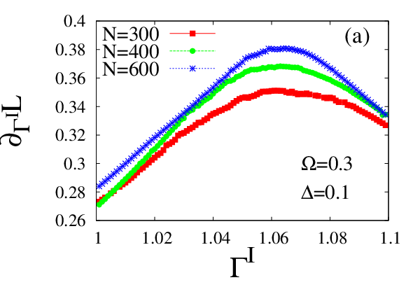
The Loschmidt echo can act as an indicator of quantum phase transition in the equilibrium [2]. This is also true for non-equilibrium situation where derivative of LE with respect to a parameter of the quantum Hamiltonian shows a singular behavior at QCP [39]. The question we ask here is that whether for a disordered chain the derivative of LE still shows a peak around the QCP of the clean chain. Our study suggests that first derivative of with respect to the transverse field shows a peak around the boundary of the Griffiths phase that is created in presence of disorder. The position of such peak does not coincide with the peak appearing at the QCP of the clean spin chain.

.


We numerically calculate the derivative of Loschmidt echo () for different values of initial transverse field by keeping final value of transverse field fixed at and time is fixed at . (see Fig.1a). The values of coupling strength and coupling distance are and respectively. In our calculation, we take disorder strength and the disorder average is made over configurations. The derivative of LE shows peak at which does not show any tendency to shift towards clean critical point () when the system size increases from to . This shift of the critical point indicates the existence of the Griffith phase in the disordered Ising spin chain; this phase arises due to the inhomogeneity of the transverse field. The derivative shows a peak at the boundary between the Griffiths phase and the disordered phase. Therefore, our numerical study indicates that the Griffiths phase is extended from the to . The analytical expression of the Griffiths phase for disorder present in both interaction and transverse field [41] might not be applicable for our case as we are dealing with randomness only in transverse field. In our case, we think that due to the disordered transverse field, the competition between spin-spin interaction and quantum fluctuation (i.e., local transverse field) are not identical in the individual sites. As result of that there exist local order in the spin chain and the thermodynamic observables essentially become non self-averaging. In this way one would expect that Griffiths phase emerges in presence of disorder transverse field. Moreover, we note that if s are distributed with only two possible values , then one would not expect to see any Griffiths phase. We also note that using fidelity susceptibility the boundary of Griffiths phase has also been probed [28]. Similar to the clean system [39], here also the peak height logarithmically increases with the system size i.e., (see Fig.1b).
III.2 Quenching dynamics of the spin chain
We numerically study the quenching dynamics of concurrence, determined by LE , between two qubits a disordered transverse field Ising chain of length . We note that in all the subsequent numerical calculation, the disorder average is made over configurations of the environmental chain and the value of coupling distance is . The nature of the coupling is determined by comparing it with the bare energy gap of the environment i.e., set by the clean spin chain with periodic boundary condition. We investigate the GCSM for strong coupling strength as well as weak coupling limit i.e., following ferromagnetic and paramagnetic quenches in the environmental spin chain. Furthermore, we extend our study of non-equilibrium dynamics of LE following a quench inside the Griffiths phase. We analyze the dynamics for different values of disorder strengths along with the clean limit . Our focus is to extensively investigate the temporal decay of LE under these different quenching schemes; we hence study the ultra-short, short and long time domains in the non-equilibrium evolution of LE.


First, we start by investigating the behavior of when the spin chain is quenched from to i.e., both the initial and the final values of transverse fields belong to the paramagnetic phase. The time evolution of for different values of are depicted in the Fig. (2a) and Fig. (2b) with weak coupling strength and strong coupling strength , respectively. For lower values of coupling strength, we find two different types of behaviors of in two different time domains (see Fig. (2a)). Initially echo for disordered chain falls of more rapidly as compared to the clean chain; the fall becomes more sharper as one increases the disorder strengths. On the other hand, in the late time limit, echo for the clean chain vanishes while for finite it remains non-zero; surprisingly, the long time value of increases with . For strong coupling case, decays more rapidly for less disordered spin chain in both the early and late time limit (see Fig. (2b)).
The initial fall is mainly determined by the difference in the initial and final Hamiltonian. In the present set up of GCSM, the weak coupling can only modify the transverse field in two sites in addition to the global sudden quench. Therefore, as one increases from , and become more deviated from each other. Hence, the overlap between the initial state i.e., eigenstate of and the time evolved state governed by Hamiltonian rapidly decays from unity. In contrary, during the course of late time dynamics the instantaneous state evolves more close to the initial state when increases; the clean chain does not lead to an instantaneous time evolved state that significantly close to the initial state. We note that the initial sharp fall is exponential while late time slow fall obeys a power law. Therefore, the advantage of having disorder in transverse field is that the qubits remain in an entangled state even long after the sudden quench. Moreover, the local details of the two Hamiltonians, governing the dynamics, are maximally determined by for strong coupling case; this results in a similar kind of fall characteristics for both early and late time limit. Disorder imprints less effects on LE for strong coupling case compared to weak coupling case.
Upon inspecting the weak and strong coupling case simultaneously, one can say that the characteristic nature of decay of LE is different for them. Although, in presence of disorder, one can see that after the initial quick fall of it decreases very slowly with time; this feature is universal for weak as well as strong coupling limit. Therefore, it is clearly evident after investigating the time evolution of LE in complete time domain that there is a crossover present in the temporal behavior.


Now, coming back to the strong coupling case where the time evolution of LE again shows the early time rapid fall and late time slow fall (see Fig. (2b)). The initial decay rate of LE for early time is higher as compared to weak coupling case. This is due to the fact that initial and final Hamiltonian become more deviated for strong coupling case. For clean system after the initial fall shows irregular oscillation which are suppressed in the presence of disorder. The late time dynamics is mainly governed by disorder strength as the decay nature of LE in small and large limit are identical.
We shall now turn our attention to the behavior of when the spin chain is quenched from the paramagnetic phase with to ferromagnetic phase with across the Griffiths phase considering (see Fig.2c) and (see Fig.2d). In this type of quenching, the initial decay rate is much higher compared to the same phase quenching as the eigenstates in the ferromagnetic side become almost orthogonal to the ground states associated with the paramagnetic phase. Unlike the quenching inside same phase, here in contrary for both type of coupling, we see that late time value of LE becomes vanishingly small. The clean system shows zero overlap after a certain time while LE for disordered system still remains finite. In case of , the values of for both pure and disordered spin chain falls drastically within a very small passage of time. Such time scale is independent of the disorder strength. For large , this time scale is much shorter and surprisingly, the clean system also decays almost identically with the disordered system. After the initial rapid fall for strong coupling case, there are oscillations in for both clean and disordered spin chain in the late time regime with very slow fall; the amplitude of oscillation for pure system is larger than the disorder spin chain. Although, such oscillations die very quickly for both types of spin chains.
Now, we shall investigate the temporal evolution of LE in different time domains following various quenching amplitudes. Let us begin with the ultra-short time analysis of the LE to investigate the fall of from unity. We numerically study ultra-short time evolution of LE for both low () and high () values of coupling strength with . For both (see Fig.(3a)) and (see Fig.(3b)) the transverse field is quenched from to the final value . In this extremely short time window, LEs for strong and weak coupling following different quench amplitudes coincide with each other.
Our numerical result shows that in both the situations, a Gaussian fall is observed within a certain time scale that depends on . The fitting of in ultra-short time window for ferromagnetic to paramagnetic quench with and are shown in Fig. (4a) and Fig. (4b), respectively. The typical characteristic time scale for is given by , whereas, in case of high values of coupling strength i.e., , the value of characteristic time is . The ultra-short time the decay of follows a Gaussian fall which can be approximated as . Here, determines the rate of the fall and the power of i.e., signifies the exponent for the Gaussian decay. We also check that this decay rate is marginally dependent of for both type of coupling. As expected, the rate for strong coupling is much higher compared to the weak coupling case. Our study further indicates that quenching inside Griffiths phase also lead to this ultra-short time Gaussian fall as depicted in Fig. (4c) for and Fig. (4d) for . Such Gaussian decay in ultra-short timescale for clean system is already observed in [39]. Therefore, one can say that the Gaussian fall observed in the ultra-short time domain remains invariant even in presence of disorder.
It has been found for a non spin preserving coupling Hamiltonian that rate for the Gaussian decay is dependent on the filling number of the ground state of the bath; specifically, exhibits plateaus as a function of intra bath coupling and transverse field [42]. Using time dependent perturbation theory it has been further confirmed analytically. The same line of argument is valid for our case also only the interaction Hamiltonian changes. Moreover, we find that is marginally dependent on disorder strength and it is evident from fig. (4) that ultra short time dynamics is mainly dictated by the initial parameter i.e., the value of transverse field. Hence, in general, one can say that strongly depends on the initial state rather than the final state. To be precise, the rate is shown to be in the form of , where is the interaction Hamiltonian between qubit and the bath, represents the expectation value with respect to the initial state of the bath [43].


At the outset, we expect that in general the decay exponent (i.e., power of ) depends on the disorder strength and the coupling strength. Upon inspecting the Fig. (5) and Fig. (6), one can remarkably see for quenching inside the same phase that for the initial small time exponential fall, the decay exponent depends only on the coupling strength; on the other hand, the decay exponent associated with the late time power law fall depends only on the disorder strength. The quenching inside a Griffiths phase as shown in Fig. (7) and Fig. (8) leads to a markedly different results in the long time regime; the power law fall is completely absent here.
In order to investigate the temporal decay of LE with disorder for the quenching inside paramagnetic phase ( to ) more extensively, we first study the initial small time rapid decay. In such time scale the double logarithm of LE becomes linear with the logarithm of time. This indicates the small time faster fall is exponential in nature. Our numerical analysis further suggests that there exist more than a single exponential fall; LE scales as and the decay exponent takes two different values in two different time regions confined within this overall exponential time zone. The decay rate is encoded in . The values of in such time domains depend on mainly. To reveal such feature, we plot with for a fixed disorder strength with several values of (see Fig.5a). Inside each characteristic region of time, two sets of parallel lines are obtained for and . For weak coupling, changes from to (see Fig.5b). In the strong coupling limit, LE continues to follow a Gaussian fall i.e., and in later time the decay exponent is close to (see Fig.5c). One can clearly observe the LE for different (for a given ) almost co-inside with each other. This refers to the fact that decay exponent does not change with the disorder strength.
We shall now focus on the late time behavior of LE for the quenching inside the paramagnetic phase. We quench the transverse filed to . We observe a late time slow power law fall of LE. Such fall can be described by , where determines the decay rate, and is the decay exponent for the power law. This late time power law decay of LE is universal for weak and strong coupling case but time domain within which this power law observed is dictated by the value of the coupling strength. To demonstrate such characteristic, we plot with for with fixed disorder strength (see Fig.6a). One can clearly find that the straight lines corresponding to different values of become parallel to each other; this suggests the power law exponent is indeed independent of coupling strength. In order to investigate dependence of , we plot the variation of with for several values keeping coupling strength fixed at (see Fig.6b) and (see Fig.6c). Irrespective of the value of coupling strength, we find that magnitude of increases with the decrease of . Moreover, we checked that the decay characteristics of LE (as described by exponential and power law fall) for quenching into a ferromagnetic phase from the paramagnetic phase remain unaltered. However, we observed a change in the extent of the time domains associated with the different types of decay.
We shall now try to justify the above numerical finding by plausible arguments. The dependent initial exponential fall is consistent with the analytical results in Refs. [44, 39]. The analytical treatments suggest the decay rate is of the order of . Therefore one would expect the initial exponential fall is dependent on coupling strength and the initial value of the transverse field rather than the disorder strength. On the other hand the asymptomatic behavior of LE depends on the final value of the quenched transverse field [44]. In a given quenching scheme, the disorder strength determines the final quenched values of transverse field at each spin site. Therefore the late time fall of LE should be governed by the disorder strength. Moreover, for strong disorder, the difference between the initial and final values of the local transverse field becomes small. As a result of that the decay of LE is severely prohibited with the increment in disorder strength. Such phenomena is exactly reflected by our numerical study associated to the late time fall of LE.


In parallel, we study the quenching inside the Griffiths phase starting from a paramagnetic phase. Similar to the paramagnetic quenching case, the initial time evolution of LE is governed by two types of exponential fall: with two different values of . The decay exponent again predominantly depends on rather than (see Fig.7a). In case of weak coupling, the LE falls off initially with and the subsequent exponential decay is accompanied with (see Fig.7b). For strong coupling case, the primary exponential fall is Gaussian with and the final exponential decay is associated with (see Fig.7c).
Most interestingly, we find that LE decays to zero in the late time limit (see Fig. (8)). This result can be contrasted to the earlier results obtained for off-critical quenching between same or different phases. In order to confirm the absence of the power law tail, logarithm of LE is plotted as a function of logarithm of time; this plot clearly depicts that logarithm of LE does not fit into a straight line within a considerable time domain. The point to note here is that as the slowly falling power tail is absent the LE decays to zero more rapidly compared to the other quenching cases. Therefore, the absence of the late time power law fall is a dynamical signature of the Griffiths phase. One can see that a tendency towards a late time slow power law fall is observed for higher values of as for some disorder realizations, environmental Ising chain lies outside the Griffiths phase.
The outcome quantum Griffiths effect is that the rare region is finite in space but infinite in imaginary time [46]; moreover, the broadening in the distribution of local relaxation time is another signature of Griffiths singularity. Consequently, the effect of the local perturbation (i.e., coupling to the qubit locally) is damped inside this huge temporal window. This might cause the initial exponential fall to prevail over the late time power law fall. The quantum Griffiths effect is absent in the PM and FM phase. The distribution of local relaxation time gets narrower leading to the fact that the effect of local perturbation is not damped completely rather it is still present in the long time. This might leads to the observation of long time power law fall of LE. This is the way we think that the characteristics of the spin chain gets imprinted the behavior of LE. Therefore, concurrence between the qubits is thus able to distinguish the phase of environmental spin chain associated with a continuously varying dynamical exponent.
Comparing the short time temporal behavior (i.e., exponential fall) of LE for different quenching case one can see that when the initial and final phases are different, LE drops most rapidly (see Fig.2c,d), while LE drops most slowly for same initial and final phases (see Fig.2a,b); for quenching into Griffiths phase from paramagnetic phase, LE attains an intermediate fall (see Fig.8). Although, the functional form of decay remains exponential, the decay rate, estimated from in , generically depends on the disorder strength, types of quenching and coupling strength. This decay rate is highest for quenching between two different phases and smallest for quenching between same phases. Moreover, this decay rate increases with increasing disorder strength in the weak coupling case. The same line of argument is also valid for decay rate associated with late time power law fall. We press the fact that disorder maximally influences the late time slow fall than the short time exponential fall, dominated by , as for the clean spin chain, LE decays to a much lower value in this late time limit. Hence, disorder imprints a positive effect in preserving an entangled state surrounded by a decohering environment.


III.3 Revival Time
In addition to the coupling strength, the dynamics of is also governed by the separation between two qubits coupled to the environmental spin chain. In this section, we discuss the dynamics of for both clean and disorder spin chain of length . Before going to the disordered chain, we shall quickly review the clean case for different values of following a quench from to as shown in Fig. (9a). We should mention that such investigation has already been made with in Ref [39] but we repeat (with different system size) this numerical calculation to present a comparative study between the observations associated to the revival of LE in pure and disordered spin chain. When the qubits are connected symmetrically i.e., , we find that echo exhibits a linear decrease till ; afterwards, of revives linearly till . As one moves away from the symmetric position by changing the separation distance from to , the time scale gradually disappears.
Concentrating on the disordered case, we show the variation of with for with several values of as depicted in Fig. (9b). One can observe that a substantial amount of disorder can wash out the above dynamical characteristics appearing in at and . The revival of LE after and the downturn at as obtained in pure case are absent in the disordered spin chain. In this case, LE monotonically decreases with time. The LE for symmetric case exhibits a higher value as compared to the non-symmetric position. In order to investigate the disappearance of singular behavior of LE, we study the LE for different disorder strength with a given . This is pictorially shown in Fig. (9c). One can see that as increases, the revival of LE at disappears, though, for small disorder strength , LE still shows a tendency of revival. This also happens for downturn time scale . For completeness, we also checked that for quenching inside the Griffiths phase, the singular time scale and completely disappear. We note that the disappearance of the singular time scale is not artifact of a particular rather it’s originated from the randomness of the transverse field.
In order to explain the disappearance of singularities, we make resort to the quasiparticle picture in the post quench regime. For the clean case, and are different from each other with respect to the local transverse fields modified at two sites, where the qubits are coupled. In the language of quasi-particle emission after a quench, one can think of two extra separate emitters, located distance away from each other. Now, in the symmetric position , quasi-particles need to travel only distance. Hence, there is a constructive interference happening that leads to a partial revival of the initial state. Therefore, with velocity of the quasiparticle . In contrast, for the disordered case, at each point, the chain experiences a change in the transverse field due to the finite value of disorder strength ; hence, separate emitters, away by a distance , do not really play a role in this global generation of quasiparticles. As an outcome of a very complicated propagation of quasiparticles from all sites, the constructive interference dies out and the appearance of the singular time scale is lost. This explanation remains true for the extinction of all the singular time scales. This is also true for quenching inside the Griffiths phase.
IV conclusion
We study the disentanglement of a Bell pair constituted of two qubits, which are connected to a disordered transverse field Ising spin chain. We identify the disorder induced Griffiths phase from the equilibrium study of LE. On the other hand from the non-equilibrium evolution of LE we exhaustively explore decay characteristics of the entanglement of the qubits and the non-trivial outcomes associated with the Griffiths phase.
In equilibrium, the derivative of LE with respect to initial transverse field is shown to exhibit a peak at critical point of the clean Ising spin chain. The disorder present only in the transverse field can lead to a local ordering in the spin chain; this results in a Griffiths phase [28] appearing at the junction of ferromagnetic and paramagnetic phases. We here numerically estimate the extent of the Griffith’s phase as the derivative of LE exhibits a peak near the boundary between Griffith’s phase and paramagnetic phase. However, such numerical evaluation of the width of the Griffiths phase needs to be verified analytically in further future studies.
From the non equilibrium study of the LE following off-critical quenches, we show that the initial fall of the LE is completely governed by the coupling strength. Such observation fairly agrees with the earlier analytical conjectures in Refs [44, 39]. Our numerical investigation suggests that the quantitative nature of the initial fall of LE cannot be explain by a single exponential function. To be precise, a ultra short time universal Gaussian fall is observed, followed by two exponential falls with two different decay exponents dependent on the coupling strength. Within this time window, the disorder is not able to reflects its effect. Since the late time fall of LE depends on the final quenched value of the transverse field [44], therefore the asymptomatic decay characteristics of LE should be controlled by the disorder strength. The increase in the value of disorder would increase the overlap between the initial and the final state of the spin chain. Therefore the initial fast exponential fall of LE is substantially suppressed by the effect of disorder in the long time limit. Consequently we observe a late time slow power law fall of LE where the value of decay exponent decreases with the increase of disorder strength. Regarding the non-trivial outcome associated with the Griffiths phase, we interestingly observe that for quenching to the Griffiths phase, the late time power law fall is completely absent while initial decay characteristics of LE is similar to that of the for the off critical quenching. Hence, the initial exponential decay is related to the initial phase, in contrary the final late time power law decay is connected to the final phase of the spin chain. Therefore, the continuous variation of the dynamical critical exponent and broadening of relaxation time mark its signature in the late time temporal profile of LE. This unique non-equilibrium characteristics of LE for the Griffiths phase might initiate further studies to identify the Griffiths phase in a disordered spin systems.
Moreover, we show that as one increases disorder strength, the singular behavior at and disappear; this is due to the fact that quasi-particles, generated from all sites, interfere destructively and the temporal structure, observed for clean system, is washed out. Hence, the linearity between distance, traveled by the quasiparticles, and time, required to travel that distance, breaks down for a substantial disorder strength. This indicates that the quasi-particles do not propagate in the light cone like fashion.
V Appendix
The anticommuting Grassmann variables are often used to compute physical quantities for example, expectation values in fermionic systems with quasifree fermion states (i.e., Gaussian states in the form of )) [45]. Specifically, the linear combinations of canonically anticommuting Fermi field operators are replaced by linear combinations of complex coefficients that are anticommuting Grassmann numbers. Based on this “Grassmann algebra of canonical anticommutation relations”, one can calculate the expectation value of with respect to the Gaussian states. The square of fidelity between two states and is given by . It has been shown that i.e., the expectation value of the support projection in the state . Using the concept of Gaussian Grassmann integral, one can show that
| (14) |
where is the phase space vector, and are two projected covariant operators associated with the states and , respectively. represents the pfaffian of a matrix. is the normalization factor, indicates the projection to initial ground state. One can use the relation to show that .
Now, connecting to the present case, and . One can consider Eq. (5) of the main text and to arrive at the above connections. We note that , being the ground state of initial Hamiltonian , is time evolved with the quenched final Hamiltonian to obtain the final states . Similarly, is the time evolved initial occupation matrix, calculated using transverse field value , with Hamiltonian . The explicit form of the covariant matrix is then given by
| (15) |
where is the initial occupation matrix composed of and . This can be computed by diagonalizing the initial Hamiltonian as stated in Eq. (8).
Acknowledgements.
The authors are grateful to Bikas K. Chakrabarti for enlightening discussion. TN thanks Kush Saha for critically reading the manuscript.References
- [1] S-J Gu, Int. J. Mod. Phys. B 24, 4371 (2010).
- [2] H. T. Quan, Z. Song, X. F. Liu, P. Zanardi, and C. P. Sun, Phys. Rev. Lett. 96, 140604 (2006).
- [3] B. Damski, H. T. Quan, W. H. Zurek, Phys. Rev. A 83, 062104 (2011).
- [4] W. K. Wootters, Qunatum Inf. Comput. I, 27 (2001), M. Horodecki, Qunatum Inf. Comput. I, 3 (2001).
- [5] M. Horodecki, Qunatum Inf. Comput. I, 3 (2001).
- [6] H. Ollivier and W. H. Zurek, Phys. Rev. Lett. 88, 017901 (2001); W. H. Zurek, Rev. Mod. Phys. 75, 715 (2003).
- [7] G. Vidal, J. I. Latorre, E. Rico, and A. Kitaev, Phys. Rev. Lett. 90, 227902 (2003).
- [8] A. Kitaev and C. Laumann, arXiv:0904.2771v1 (2009),
- [9] T. Nag, U. Divakaran and A. dutta, Phys. Rev. B, 86 020401 (R) (2012).
- [10] R. Sachdeva, T. Nag, A. Agarwal, and A. Dutta, Phys. Rev. B 90, 045421 (2014).
- [11] S. Suzuki, T. Nag and A. Dutta, Phys. Rev. A, 93, 012112(2016).
- [12] T. Nag, Phys. Rev. E 93 062119 (2016).
- [13] T. Nag, and A. Dutta, Phys. Rev. A 94, 022316 (2016).
- [14] A. Rajak, and U. Divakaran, JSTAT 043107 (2016).
- [15] B. K. Chakrabarti, A. Dutta and P. Sen, Quantum Ising Phases and transitions in transverse Ising Models, m41 (Springer, Heidelberg,1996).
- [16] S. Sachdev, Quantum Phase Transitions(Cambridge University Press, Cambridge, England,1999).
- [17] A. Polkovnikov, K. Sengupta, A. Silva and M. Vengalattore, Rev. of Mod. Phys. 83, 863 (2011).
- [18] A. Dutta, G. Aeppli, B. K. Chakrabarti, U. Divakaran, T. Rosenbaum and D. Sen, Quantum Phase Transitions in Transverse Field Spin Models: From Statistical Physics to Quantum Information (Cambridge University Press, Cambridge, 2015).
- [19] F. M. Cucchietti, J. P. Paz and W. H. Zurek, Phys. Rev. A 72, 052113 (2005); F. M. Cucchietti, S. Fernandez-Vidal, J. P. Paz, Phys. Rev. A 75, 032337 (2007); Z. -G. Yuan, P. Zhang and S. -S. Li, Phys. Rev. A 76 042118 (2007).
- [20] Z. G. Yuan, P. Zhang and S. -S. Li, Phys. Rev. A 76, 042118 (2007), R. Jafari and H. Johannesson Phys. Rev. Lett. 118, 015701 (2017), R. Jafari and H. Johannesson Phys. Rev. B 96, 224302 (2017).
- [21] J. Zhang, F. M. Cucchietti, C. M. Chandrashekar, M. Laforest, C. A. Ryan, M. Ditty, A. Hubbard, J. K. Gamble, and R. Laflamme, Phys. Rev. A 79, 012305 (2009).
- [22] D. S. Fisher, Phys. Rev. Lett. 69, 534 (1992); Phys. Rev. B 51, 6411 (1995).
- [23] C. Dasgupta and S.-K. Ma, Phys. Rev. B 22, 1305 (1980).
- [24] F. Igloi and C. Monthus, Phys. Rep. 412, 277 (2005).
- [25] R.H. McKenzie, Phys. Rev. Lett. 77, 4804 (1996).
- [26] J.E. Bunder, R.H. McKenzie, Phys. Rev. B 60, 344 (1999).
- [27] R.B. Griffiths, Phys. Rev. Lett 23, 17 (1969).
- [28] S. Garnerone, N.T. Jacobson, S. Haas, and P. Zanardi, Phys. Rev. Lett., 102, 057205 (2009). N. T. Jacobson, S. Garnerone, S. Haas, and P. Zanardi, Phys. Rev. B 79, 184427 (2009)
- [29] I. Peschel, J. Phys. A: Math. Gen. 38, (2005) 4327–4335.
- [30] G. Refael and J. E. Moore, Phys. Rev. B 76, 024419 (2007).
- [31] R. Juhasz, I. A. Kovacs and F. Igloi, Euro. Phys. Lett, 107, 47008 (2014), I. A. Kovacs, R. Juhasz, and F. Igloi, Phys. Rev. B 93, 184203 (2016).
- [32] H. Li, J. Wang, X-J Liu, H. Hu, Phys. Rev. A 94, 063625 (2016).
- [33] W. H. Zurek, U. Dorner, and P. Zoller, Phys. Rev. Lett. 95, 105701 (2005); A. Polkovnikov, Phys. Rev. B 72, 161201(R) (2005).
- [34] K. Sengupta and D. Sen, Phys. Rev. A 80, 032304 (2009), T. Nag, A. Patra and A. Dutta, Jour. Stat. Mech. (2011), P08026; S. Suzuki, T. Nag and A. Dutta, Phys. Rev. A 93, 012112 (2016).
- [35] T. Nag, A. Dutta and A. Patra, Int. J. Mod. Phys. B 27, 1345036, (2013).
- [36] F. Igloi, Z. Szatmari, and Y. -C. Lin, Phys. Rev. B 85, 094417 (2012).
- [37] J. A. Kjall, J. H. Bardarson, and F. Pollmann, Phys. Rev. Lett. 113, 107204 (2014).
- [38] S. Ziraldo, A. Silva and, G. E. Santoro, Phys. Rev. Lett. 109, 247205 (2012), S. Ziraldo and, G. E. Santoro, Phys. Rev. B 87, 064201 (2013).
- [39] P. Wendenbaum, B. Taketani and D. Karevski, Phys. Rev. A 90, 022125 (2014).
- [40] C. Cormick and J. P. Paz, Phys. Rev. A 78, 012357 (2008), Z. Sun, X. Wang, and C. P. Sun, Phys. Rev. A 75, 062312 (2007).
- [41] A. P. Young and H. Rieger, Phys. Rev. B 53, 8486 (1996).
- [42] N. Wu, A.Nanduri, and H. Rabitz, Phys. Rev. A 89, 062105 (2014).
- [43] A. Peres, Phys. Rev. A 30, 1610 (1984).
- [44] D. Rossini, T. Calarco, V. Giovannetti, S. Montangero, and R. Fazio Phys. Rev. A 75, 032333 (2007).
- [45] M. keyl and D-M. Schlingemann, J. Math. Phys. 51, 023522 (2010).
- [46] M. Vojta, J. A. Hoyos, Phys. Rev. Lett. 112, 075702 (2014).