A dynamical approach in exploring the unknown mass in the Solar system using pulsar timing arrays
Abstract
The error in the Solar system ephemeris will lead to dipolar correlations in the residuals of pulsar timing array for widely separated pulsars. In this paper, we utilize such correlated signals, and construct a Bayesian data-analysis framework to detect the unknown mass in the Solar system and to measure the orbital parameters. The algorithm is designed to calculate the waveform of the induced pulsar-timing residuals due to the unmodelled objects following the Keplerian orbits in the Solar system. The algorithm incorporates a Bayesian-analysis suit used to simultaneously analyse the pulsar-timing data of multiple pulsars to search for coherent waveforms, evaluate the detection significance of unknown objects, and to measure their parameters. When the object is not detectable, our algorithm can be used to place upper limits on the mass. The algorithm is verified using simulated data sets, and cross-checked with analytical calculations. We also investigate the capability of future pulsar-timing-array experiments in detecting the unknown objects. We expect that the future pulsar timing data can limit the unknown massive objects in the Solar system to be lighter than to , or measure the mass of Jovian system to fractional precision of to .
Keywords:
pulsar:general – minor planets, asteroids: general – methods: data analysis1 Introduction
The clock-like rotational stability of millisecond pulsars makes them the the most accurate celestial clocks known. Through the process of pulsar timing (Lorimer & Kramer, 2005; Hobbs et al., 2006, e.g.), millisecond pulsars are powerful tools for a wide range of scientific problems. In the process of pulsar timing, the time of arrivals (TOAs) recorded at the observatory are transferred to the pulsar frame. The differences between the observed TOAs and the model predictions form the timing residuals. The physical processes not modelled will leave their fingerprints in the timing residuals. For processes affecting all the pulsars, they introduce the correlated signals between widely separated pulsar pairs. Such spatial correlations have profound applications. For example, one can detect the gravitational waves (Hellings & Downs, 1983, GW;), investigate the stability of reference terrestrial time standards (Hobbs et al., 2012), and study the Solar system ephemeris (Champion et al., 2010). These applications make use of so-called pulsar timing arrays (PTAs), which are an ensemble of pulsars, typically millisecond pulsars, in different sky positions (Foster & Backer, 1990).
The first step in converting the site TOAs to the pulse-emission time at the pulsar frame, is to refer them to the Solar system barycentre (SSB) according to the SSB position with respect to the Earth. In the common pulsar timing practice, the SSB position is provided by the Solar system ephemeris (Standish, 1998). Errors in the used ephemeris will then lead to inaccurate conversion of TOAs, and thus induce the correlated timing residuals among all analysed pulsars. We can study the Solar system ephemeris by searching for such correlated residuals.
Champion et al. (2010) were the first to employ a PTA to constrain the mass of planets in the Solar system . They fixed the orbits of the known planets using the DE421 ephemeris (Folkner et al., 2009) and investigated the effects of perturbing the input planetary masses on the TOAs. In this way, they used the PTA data to constrain possible errors in the Solar system ephemeris, and provide upper limits on the masses of planets (or planetary systems when satellites are in orbit).
Possible errors in the Solar system ephemeris may come from two aspects: inaccurate mass or position of known objects, and the existence of unmodelled objects (UMOs). Champion et al. (2010) had studied the error in the mass of known planets. In this paper, we want to explore the unknown objects in the Solar system by pulsar timing, to detect their signal or put upper limits on their masses. The term UMOs here refers to any unknown objects revolving around the SSB, such as dark matter clumps (Loeb & Zaldarriaga, 2005; Pitjev & Pitjeva, 2013), small asteroids (Sheppard & Trujillo, 2016), strangelets (Wu et al., 2007), cosmic strings (Blanco-Pillado et al., 2014), tiny primordial black holes or other unidentified massive objects. The studies of timing residuals induced by the ephemeris can help us understand the noise budget of PTAs, which is of central importance for the GW detection with PTAs. Furthermore, a better Solar system ephemeris may also improve the precision of deep space missions.
In the current paper, we model the UMOs with Keplerian orbits, calculate the induced timing residuals, and perform parameter estimation using Bayesian inference. We describe our methods in Section 2, and use simulations to verify our algorithm in Section 3. We analytically calculate the PTA sensitivity to the UMOs and investigate the capability of future PTA experiments in Section 4. Discussions and conclusions are made in Section 5.
2 Methods
We use a model-based Bayesian data-analysis method to measure the mass of UMOs using PTA data. There are two major components for the Bayesian inference, the signal model (in Section 2.1) and the likelihood model (in Section 2.2).
2.1 Pulsar-timing residuals induced by UMOs
Pulsar timing residuals can be described as the sum of three sources: the signal , induced by unmodelled processes such as the orbit of a UMO, the signal , induced by imperfectly modelled timing parameters, and the signal , from noise processes. That is
| (1) |
In most of the pulsar-timing procedures, one uses the clock corrections published by the Bureau International des Poids et Mesures (BIPM)11 1 http://www.bipm.org/, Earth orientation parameters and Solar system ephemeris to correct the TOAs seen at the telescope site to the TOAs as seen in the pulsar rest frame. In this way, any objects not included in the ephemeris will introduce signals in the pulsar timing residuals. Such signals have a dipolar spatial correlation, different from the monopolar correlation induced by clock errors (Hobbs et al., 2012). In this paper, we focus on the leading-order effects of the UMOs under the following two assumptions.
(i) We assume that the UMO follows a point-mass Keplerian orbit around the SSB. In particular, we focus on bound systems, of which orbits are elliptic. The major acceleration of the UMO is thus due to the Sun, and we neglect the higher-order effects, such as the perturbations from objects except the Sun in the Solar system, the post-Newtonian corrections, and tidal forces.
(ii) The UMOs induce periodic motion of the SSB. Such motion will contribute to the pulsar-Earth distance and lead to an extra geometric time delay in the pulsar TOAs (i.e. the Rømer delay as explained in Edwards et al. (2006)). We have neglected the higher-order effects due to the SSB motion (e.g. parallax, gravitational redshifts, and Shapiro delay), as done by Champion et al. (2010).
Champion et al. (2010) showed that the perturbation of Jupiter mass simply changes the position of the SSB, as we modelled. It is unclear if such perturbative approach is also valid for the other planets, especially the ones with inner orbits. Investigating the long-term evolution of the Solar system dynamics with full modelling is beyond the scope of this article. However, the data length is limited to only a couple of tens of years, such that the first-order treatment, i.e. UMOs induce SSB shifts, is a valid approximation.
The Røemer delay associated with the displacement of the SSB is
| (2) |
where is the unit vector pointing to the direction of the pulsar, and is the speed of light. As we neglected the interaction between UMO and other Solar system objects other than the Sun, the displacement of the SSB caused by the UMO with mass and position vector relative to the original SSB is
| (3) |
where is the total mass of the Solar system and can be well approximated by the solar mass, such that .
The Keplerian orbit of a UMO is modelled with seven parameters (), which fully determine the induced pulsar-timing residuals. The parameters contain the mass of the UMO and six orbital elements. The orbital elements determine the geometry of orbit, and are the semi-major axis, , eccentricity, , longitude of the ascending node, , orbital inclination angle, , argument of perihelion , and phase at reference epoch, .
For elliptic orbits, the radial distance of a UMO to the centre of mass, , can be expressed in terms of the eccentric anomaly, , as
| (4) |
The evolution of with time satisfies
| (5) |
where is the orbital frequency. The latter follows Kepler’s third law, such that
| (6) |
Using the true anomaly , the position vector of the UMO in the orbital plane becomes
| (7) |
and the true anomaly is defined as
| (8) |
We transform the position vector to the ecliptic coordinate using rotation matrix as computed from the Euler angles of orbital elements, such that
| (9) | |||||
| (10) | |||||
| (11) |
The dependence of the timing residuals, , on the timing parameters, , is usually non-linear, but the timing model can be linearized around the reference timing parameters, , to compute the timing residuals (Manchester & Taylor, 1977; Lorimer & Kramer, 2005; Edwards et al., 2006; van Haasteren et al., 2009), which leads to
| (12) |
Here, is the index of each epoch of observation, and is an index for the timing parameter. is the design matrix (the coefficients of linearization), and is the deviation of timing parameters from the reference values.
Unlike the deterministic signal and , the noise components, , in the timing residuals are random. We model them through the likelihood function as described in the next section.
2.2 The likelihood function and Bayesian inference
We perform the parameter estimation using Bayesian inference. The Bayesian techniques had been studied extensively in the field of pulsar timing (van Haasteren et al., 2009; Lee et al., 2014; Caballero et al., 2016; Lentati et al., 2016). Bayesian inference relies on converting the ‘probability of data’ to the ‘probability of parameters’ using Bayes’ theorem,
| (13) |
where is the data, and are the parameters to be inferred. is the likelihood function, i.e. the probability density function for the data given the parameters. is the posterior probability distribution, i.e. the probability density function for the parameters given the data set. The Bayesian evidence is a normalization coefficient, defined as
| (14) |
The prior probability distribution describes a priori belief about the distribution of the model’s parameters.
In the current paper, we assume the random noise in pulsar-timing residual of individual pulsars is a zero-mean Gaussian process. This approach had been taken by many authors. We refer the interested readers to Lee et al. (2014) or Caballero et al. (2016) for the details of single-pulsar noise modelling. Here we only briefly outline the definitions.
Under the Gaussian assumption the noise components can be fully characterized using the covariance matrix, C,
| (15) |
where is the number of data points, refers to the noise model parameters, and symbols , -1, and are the determinant, inversion, and transpose operation for matrices, respectively.
The noise processes in pulsar timing, are usually classified into three major parts, white-noise, red-noise, and the frequency-dependent-noise processes (see Cordes, 2013, for a review). In this paper, we focus on the first two, the white noise and red noise. The noise power is additive, if the white noise and red noise are uncorrelated. The noise covariance matrix becomes .
The white noise is modelled as the TOA uncertainty scaled by a systematic factor (‘Efac’) , with determined by the template fitting of pulse profile (Hotan et al., 2004). We also include a possible independent source of white noise (such as jitter) which is modelled by Equad. The white noise covariance matrix becomes
| (16) |
The red noise is modelled as a wide-sense stationary Gaussian stochastic signal with a power-law spectrum (Lee et al., 2014),
| (17) |
where is a reference frequency, and is the data length. The Fourier transform of the spectral density gives the temporal correlation of the red noise,
| (18) |
where is the time difference between the -th and -th epoch.
With all the ingredients, the likelihood function for the UMO problem is
| (19) | |||||
The parameters that we are interested in are the orbital elements . We can marginalise the likelihood function over the other parameters, which are referred to as “nuisance parameters”. The timing model parameters are linear, and they can be marginalised analytically (van Haasteren et al., 2009) giving
| (20) |
with
| (21) | |||||
| (22) | |||||
| G | (23) |
where M is the number of timing model parameters.
The noise parameters in are nonlinear, and their marginalisation can only be performed numerically. We marginalise them in the stage of stochastic sampling of the posterior. In this way, we fit the orbital elements and noise parameters simultaneously, with the parameters of timing model marginalised analytically.
Besides the likelihood function, the Bayesian analysis also depends on the prior distribution . For the parameter estimation, one should use the least informative prior, the Jeffreys prior (Gregory, 2005). The prior distributions are uniform for dimensionless parameters, while uniform in the log-space for the parameter with dimension. However, the logarithmic prior introduces an infinite-volume parameter space close to the origins, which makes the confidence level of upper limits invalid. As a consequence, the use of uniform priors is required to place reasonable upper limits (Caballero et al., 2016; Lentati et al., 2016).
In the following sections, we demonstrate our method by analysing simulated data sets. The sampling of posterior is carried out using the nested-sampling Monte Carlo algorithm multinest (Feroz et al., 2009). A paper where the presented method is applied to the first International Pulsar Timing Array data (Verbiest et al., 2016), is now in preparation.
3 Demonstration and verification
We simulate timing data for five pulsars from the IPTA pulsar list (Verbiest et al., 2016), namely PSRs J04374715, J10125307, J17130747, J19093744 and J21450750. These pulsars have the lowest level of timing residuals and cover a wide distribution on the sky, so are suitable for our algorithm verification. The parameters of timing noise injected in the simulated data are listed in Table 1, where the timing precisions are from the root-mean-square values of residuals in Verbiest et al. (2016). The properties of the red noise are consistent with the values in Caballero et al. (2016) and Lentati et al. (2016). We simulate the data with a cadence of two weeks and total length of ten years.
| PSR | ) | ||
|---|---|---|---|
| J04374715 | 0.3 | 0.08 | -0.41 |
| J10125307 | 1.7 | 0.20 | -0.21 |
| J17130747 | 0.3 | 0.09 | -0.40 |
| J19093744 | 0.2 | 0.02 | -0.11 |
| J21450750 | 1.2 | 0.31 | -0.02 |
We address two scenarios here,
case 1 If there are no detectable UMOs, we derive upper limits on their masses.
case 2 If the UMO signal is strong, we measure their orbital elements.
We use the following recipe to simulate our data.
- 1.
Simulate the perfect TOAs for each pulsar using tempo2.
- 2.
Add the white and red noise according to the noise parameters, where the red noise is synthesised from the given spectrum using the fine frequency grid of .
- 3.
For case 2, we inject the UMO induced signal.
Data analysis and results of case 1. In this case, the UMO signal is not injected. We use Bayesian techniques to derive the upper limit for the mass of UMO. The timing residuals of the simulated data set are plotted in Figure 1.
Our data analysis consists of two major steps. In the first step, we quantify if we detect the UMO, while in the second step, we perform parameter inference. We use Bayes factor () to evaluate the detection significance. To do so, we need two Bayesian samplings, one using the model including only the noise parameters and the other one using the model including both noise parameters and UMO parameters. Then the Bayes factor is the ratio between the Bayesian evidence of the two model. For the data in Figure 1, we get . Based on the interpretation of the Bayes factor by Kass & Raftery (1995), this is an indication that the simpler model without the presence of UMO signals is preferred, and so this allows us with confidence to assume non-detection for this data set and proceed to the next step.
In the second step, we focus on getting the upper limit for the mass of UMOs. It is more informative to know such upper limits as function of the semi-major axis (). We therefore go through a grid of semi-major-axis values and perform upper-limit inference. For each value of , we perform posterior sampling for the rest of the orbit and noise parameters. Using a uniform prior on the mass of UMO, we derive its upper limit. An example of the posterior distribution for a search for UMOs at is shown in Figure 2. The corresponding upper limits of the UMO mass as a function of the semi-major axis is presented in Figure 3. As one can see, with this simulated data set, any UMO with mass above should be excluded within of the SSB. The spike at is caused by fitting for the position of the pulsar. This removes any sinusoidal component with an annual period, while the much smaller spike with a half-year period () results from fitting for parallax, which removes only a sinusoidal component in phase with the Earth’s orbit. The reduction in sensitivity for periods longer than 7 years is due to fitting for the pulse period and spin-down rate, as will be discussed in Section 4.

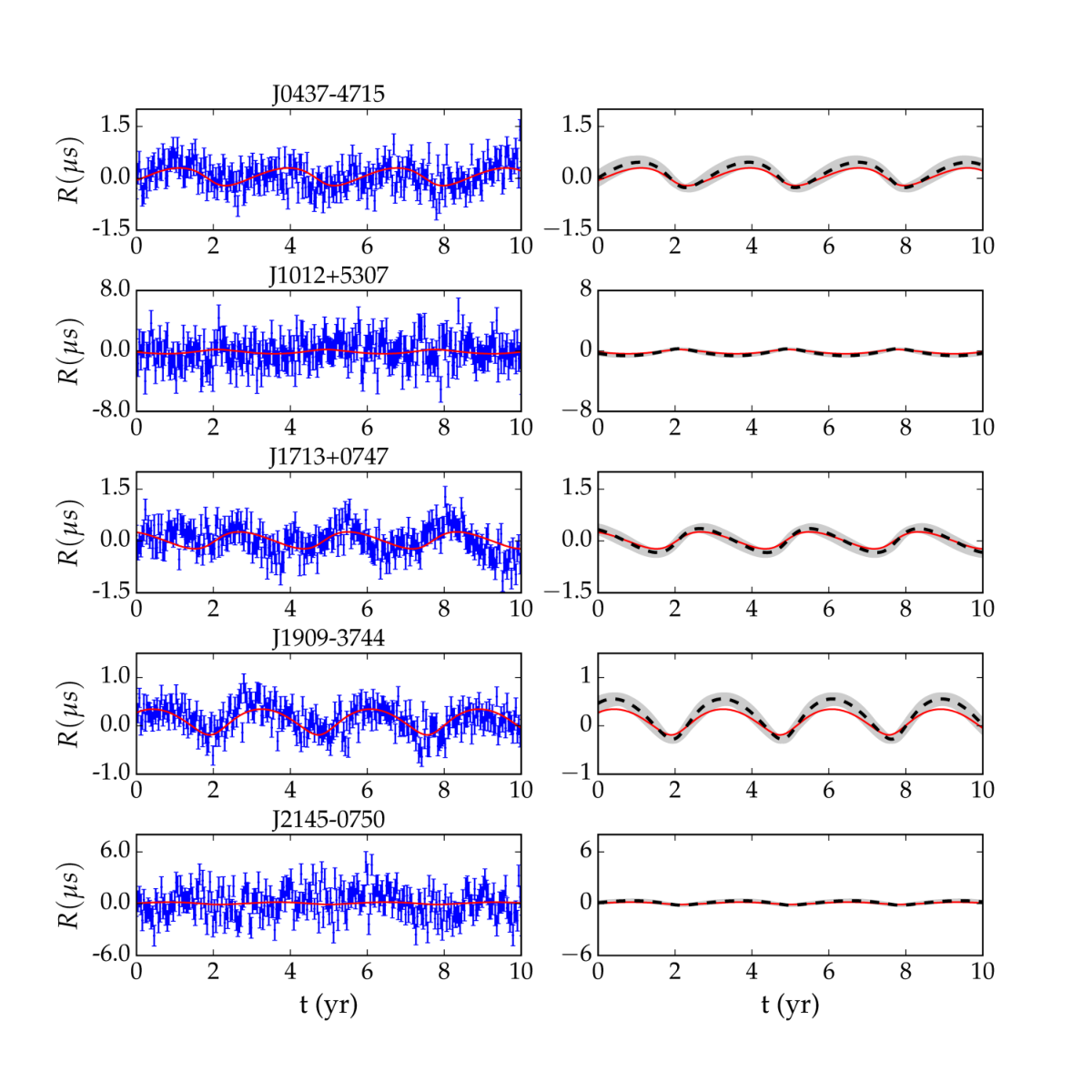
Data analysis and results of case 2. In this case, we inject the signal of a UMO in the simulated data set and demonstrate the method to measure the parameters of UMO. For the UMO signal, the semi-major axis is chosen to be AU. The mass is , i.e. at the upper limit of case 1. A moderate value of 0.3 is selected for the eccentricity. While this value is actually larger than any other planets in the Solar system, we choose it to verify the ability of searching for eccentric orbit. The remaining angle parameters are set arbitrarily to be 1 radian. Table 2 lists those parameters. The injected UMO signal and simulated data are in Figure 4.
As in case 1, we computed the Bayes factor and found that , which, again based on Kass & Raftery (1995), is a clear preference for the model that includes an UMO. The posterior distribution for the parameter inference is shown in Figure 5. As a comparison, we overplot the reconstructed waveforms using the inferred parameters along with the injected signals in Figure 4. From these figures, one can see that for strong signals, the current algorithm produces compatible UMO parameters compared with the injection values.
| Parameter | Simulation | Inference |
|---|---|---|
| -9.3 | ||
| /AU) | 0.3 | |
| 0.3 | ||
| 1 | ||
| 1 | ||
| 1 | ||
| 1 |
4 Analytical results and future perspectives
In this section, we derive the analytic formula for the mass upper limit of the UMO. We verify the analytic formula using simulations and then use the analytic results to investigate the capability of future PTA experiments in detecting the UMOs.
4.1 Analytic formula
The Cramér-Rao bound is a well-studied statistical tool (Fisz, 1963) to determine the lowest bound on the variances of estimators. It can be regarded as the upper limits for the none detection, or the errorbar when the parameter is measured. Given the likelihood function, , the expected covariance matrix of parameter error is
| (24) |
Here, the model parameters are described by the vector . They contain both the timing parameters and the UMO parameters . For the Gaussian likelihood, i.e. equation (19), the above Cramér-Rao bound can be reduced to (Slepian, 1954)
| (25) |
To proceed, we further simplify the problem by considering only white noise contribution and we assume that (1) the eccentricity of the UMO is small, i.e. , and that (2) there are enough data points such that . The first assumption helps to get a closed form for the UMO induced signal, . Under the second assumption, we can replace the summation of matrix indices in equation (25) with the continuous time integration. We then get,
| (26) |
For the mass of UMO, equation (26) leads to an analytical expression at the two following limits of the semi-major axis:
| (27) |
where is the effective root-mean-square level of pulsar noise,
| (28) |
In the above equations, is the average number of observation epochs per pulsar, is the average length of observation, and is the sky sensitivity. The latter is the geometric correction factor for taking into account the projection of the signal to the pulsar direction, as in equation (2). The sky sensitivity, , approaches unity, when the number of pulsars, . For limited number of pulsars, can be treated as a factor of 2, as we do for the case of five pulsars in our analysis. The sensibility of this approximation can be illustrated by plotting the value of for the five pulsars we used as shown in Figure 6.

In equation (27), there are two cases depending on the value of . For the case of a small , the frequency of the UMO signal is high such that the UMO signal and the quadratic pulsar spin-down signal are uncorrelated. The error of UMO mass is inversely proportional to because of equation (3), and in this regime, the UMO located farther to the SSB is easier to detect. In the second regime, when becomes larger, the data span is not long enough to cover several orbital periods, so the short-duration sinusoidal function is correlated with the quadratic pulsar spin-down signal. The UMO signal is no longer periodic in the data. The dependence comes from the cubic function left in the residuals due to the fitting of pulsar period and period derivative.
To assess the predictive power of equation (27), we employ it to calculate analytically the UMO-mass sensitivity curves for the case 1 simulations and compare it with the results from the Bayesian analysis. The results are shown in Figure 7. One can see that such an analytical expression, although much simplified, still encapsulates the major features of the sensitivity curve. The deviations between the analytical expression and the numerical results become significant, when is large. In this regime, the UMO orbital period is larger than the data length, and the estimations of mass upper limit become highly affected by the choice of prior and red noise modelling. The analytical expression gives the correct power index, i.e. , but the numerical factor becomes less reliable.
The Cramér-Rao bound will fail for the situation, when a unique un-biased estimator is not available (Lee et al., 2011). For the current UMO problem, this happens, when the number of pulsars is limited. In certain cases, a limited number of pulsars have much better precision than the rest of pulsars in the timing array. This effectively reduces the number of pulsars contributing to the analysis. We show an ill-conditioned example in Figure 8, and the corresponding posterior distributions from the Bayesian analysis in Figure 9. Although the recovered waveform is very different for PSR J21450750, the timing precision limits us from differentiating the two sets of parameters. In general, three parameters can be measured from the signal of one pulsar, namely the amplitude, frequency and phase. We will need more than three pulsars to measure the seven parameters describing the UMO.
4.2 Prediction
In the near future, discoveries of more stable millisecond pulsars and new commissions of advanced instruments will continuously increase the quality of pulsar-timing data. The Five-hundred-meter Aperture Spherical radio Telescope (Nan et al., 2011, FAST;), the QiTai 110m radio Telescope (Wang, 2017, QTT;) and the Square Kilometre Array (Kramer & Stappers, 2010, SKA;), will significantly improve the timing precision for a large number of pulsars. We expect the upper limit for the UMO mass will be more stringent.
We estimate the future upper limits of the UMO mass using equation (27), and the results are summarized in Figure 10. One can see that with 10-year pulsar timing for 20 pulsars to the precision of 100 ns, we can push the mass upper limits to to , i.e. to Jupiter mass. Other cases show the improvement of upper limits with longer data span, more pulsars and increased precision. The upper limits can be an order of magnitude better, if we use 20-year data of 20 pulsars with a precision of 30 ns. Since the timing precision of 30 ns over 20 years is unlikely due to noise processes in pulsars, the result will probably look that good only for UMOs with periods of years. The upper limit is also the precision of measurements, so we expect that future PTAs will measure the mass of Jovian system with a fractional precision of to , which is comparable to the existing IAU uncertainties (Luzum et al., 2011).
5 Discussions and Conclusions
We have developed a method to search for UMOs in the Solar system using PTA data. Our algorithm is based on the Bayesian data-analysis framework, where the detection significance is evaluated using Bayes factor and the parameter inference is performed using posterior sampling. We have verified the method using simulated data sets. The current method is capable of producing the upper limit for the mass of UMOs and to measure the orbit elements. As we have demonstrated, the parameter inference matches the injection values in the simulation. We have also derived the analytical expression for the upper limits of UMO mass. The upper limits using the Bayesian inference agree well with our analytical expression. With this method, we have estimated the future perspectives of detecting the UMOs using pulsar timing array. The method has different selection effects compared to the traditional planet detections, e.g. optical surveys, that even the invisible exotic objects can be detected, as long as they are massive.
Champion et al. (2010) measured the mass error of the known planets, based on the Solar system ephemeris DE421. By employing a dynamical model for the orbit, our method measures the properties of UMOs, both the mass and orbital elements. The Bayesian framework helps to simultaneously analyze the signal of UMOs, pulsar timing model in the presence of other noise processes. We have assumed Keplerian orbits for the UMOs and neglected all perturbations. Here, the assumption saves us from implementing the full dynamic modelling of Solar system as in Seidelmann (2005). In our model, we neglect all propagation effects of pulsar signal due to the UMO other than Rømer delay. The higher order terms, e.g. Shapiro delay and gravitational red shift of UMO, will be not be measurable for objects much lighter than the Jupiter. While obviously having the advantage of fully exploring the orbital parameters, the method is currently practically limited to study light objects not in orbit with other planets. Nevertheless, the algorithm presented can serve as a basis on which we can found attempts to perform full dynamical modelling in the future. It is noteworthy that inaccuracies in the used Solar system ephemeris, are identified as one of the main sources of correlated noise in PTA data that impede efforts for direct nHz GW detections (Tiburzi et al., 2016; Taylor et al., 2017; Wang et al., 2017, e.g.). Modelling approaches such as the one presented in this work, can help in efforts to mitigate this noise and improve the PTA sensitivity to GWs (Lentati et al., 2015; Li et al., 2016). We also note, that while discoveries of previously unknown bodies in the solar system with PTA blind searches may be difficult, the use of more evolved dynamical models may allow in the future PTAs to contribute in imposing meaningful constraints on the parameter space of independently proposed unknown planets (Batygin & Brown, 2016; Brown & Batygin, 2016, e.g.), as shown in Figure 10.
Both the pulse period and period derivative are fitted in the timing model, which absorbs the linear and quadratic signals. In this way, our method is not sensitive to the acceleration of the Solar system, and it searches for the ‘jerk’ in the timing signal for long-period planets, i.e. we search for the time derivative of Solar system acceleration for the second case in equation (27). There are works to constrain the Solar system acceleration directly. Zakamska & Tremaine (2005) proposed to detect the Solar system acceleration using distribution of millisecond pulsars (under the assumption of position-independent distribution) or orbital period derivative of binary pulsars. Verbiest et al. (2008) and Deller et al. (2008) timed the binary PSR J04374715 and determined the upper limit of Solar system acceleration using orbital period derivative.
Our analytical expression for the mass upper limit is derived using Cramér-Rao bound. Since it theoretically predicts the best possible upper limit for any unbiased estimator, it is a very useful tool to cross check the data-analysis as well as to make predictions to help planning future observations. As we see, timing 20 pulsars to the precision of 100 ns, will rule out any unknown objects with mass of to within 10 AU around the Sun. For dark matter clumps, this will be a factor of better than the current limit (Pitjev & Pitjeva, 2013; Pitjeva & Pitjev, 2013). The PTAs become sensitive tools to study the Solar system mass distribution and dynamics. We expect that advanced instruments (e.g. FAST, SKA, and QTT) in the future will benefit the field.
Acknowledgments
This work was supported by XDB23010200, National Basic Research Program of China, 973 Program, 2015CB857101 and NSFC U15311243, 11690024, 11373011. We are also supported by the MPG funding for the Max-Planck Partner Group. The computation was performed using the cluster Dirac in KIAA and the Tianhe II supercomputer at Guangzhou supported by Special Program for Applied Research on Super Computation of the NSFC-Guangdong Joint Fund (the second phase) under Grant No.U1501501. We thank Joris Verbiest, William Coles and Stephen Taylor for helpful comments.
References
- Batygin & Brown (2016) Batygin K., Brown M. E., 2016, AJ, 151, 22
- Blanco-Pillado et al. (2014) Blanco-Pillado J. J., Olum K. D., Shlaer B., 2014, Phys. Rev. D., 89, 023512
- Brown & Batygin (2016) Brown M. E., Batygin K., 2016, ApJ, 824, L23
- Caballero et al. (2016) Caballero R. N., et al., 2016, MNRAS, 457, 4421
- Champion et al. (2010) Champion D. J., Hobbs G. B., Manchester R. N., et al., 2010, ApJL, 720, L201
- Cordes (2013) Cordes J. M., 2013, Classical and Quantum Gravity, 30, 224002
- Deller et al. (2008) Deller A. T., Verbiest J. P. W., Tingay S. J., Bailes M., 2008, ApJ, 685, L67
- Edwards et al. (2006) Edwards R. T., Hobbs G. B., Manchester R. N., 2006, MNRAS, 372, 1549
- Feroz et al. (2009) Feroz F., Hobson M. P., Bridges M., 2009, MNRAS, 398, 1601
- Fisz (1963) Fisz M., 1963, Probability Theory and Mathematical Statistics . New Yorker: Wiley
- Folkner et al. (2009) Folkner W. M., Williams J. G., Boggs D. H., 2009, Interplanetary Network Progress Report, 178, 1
- Foster & Backer (1990) Foster R. S., Backer D. C., 1990, ApJ, 361, 300
- Gregory (2005) Gregory P. C., 2005, Bayesian Logical Data Analysis for the Physical Sciences: A Comparative Approach with ‘Mathematica’ Support. Cambridge University Press
- Hellings & Downs (1983) Hellings R. W., Downs G. S., 1983, ApJL, 265, L39
- Hobbs et al. (2012) Hobbs G., Coles W., Manchester R. N., et al., 2012, MNRAS, 427, 2780
- Hobbs et al. (2006) Hobbs G. B., Edwards R. T., Manchester R. N., 2006, MNRAS, 369, 655
- Hotan et al. (2004) Hotan A. W., van Straten W., Manchester R. N., 2004, PASA, 21, 302
- Kass & Raftery (1995) Kass R. E., Raftery A. E., 1995, Journal of the american statistical association, 90, 773
- Kramer & Stappers (2010) Kramer M., Stappers B., 2010, in ISKAF2010 Science Meeting - ISKAF2010, June 10-14, 2010 Assen, the Netherlands LOFAR, LEAP and beyond: Using next generation telescopes for pulsar astrophysics . p. 10
- Lee et al. (2014) Lee K. J., Bassa C. G., Janssen G. H., Karuppusamy R., Kramer M., Liu K., Perrodin D., Smits R., Stappers B. W., van Haasteren R., Lentati L., 2014, MNRAS, 441, 2831
- Lee et al. (2011) Lee K. J., Wex N., Kramer M., Stappers B. W., Bassa C. G., Janssen G. H., Karuppusamy R., Smits R., 2011, MNRAS, 414, 3251
- Lentati et al. (2016) Lentati L., Shannon R. M., Coles W. A., et al., 2016, MNRAS, 458, 2161
- Lentati et al. (2015) Lentati L., Taylor S. R., Mingarelli C. M. F., et al., 2015, MNRAS, 453, 2576
- Li et al. (2016) Li L., Guo L., Wang G.-L., 2016, Research in Astronomy and Astrophysics, 16, 58
- Loeb & Zaldarriaga (2005) Loeb A., Zaldarriaga M., 2005, Phys. Rev. D., 71, 103520
- Lorimer & Kramer (2005) Lorimer D., Kramer M., 2005, Handbook of Pulsar Astronomy. Cambridge Univ. Press, Cambridge, UK
- Luzum et al. (2011) Luzum B., Capitaine N., Fienga A., Folkner W., Fukushima T., Hilton J., Hohenkerk C., Krasinsky G., Petit G., Pitjeva E., Soffel M., Wallace P., 2011, Celestial Mechanics and Dynamical Astronomy, 110, 293
- Manchester & Taylor (1977) Manchester R. N., Taylor J. H., 1977, Pulsars.. W. H. Freeman, San Francisco, CA, USA
- Nan et al. (2011) Nan R., Li D., Jin C., Wang Q., Zhu L., Zhu W., Zhang H., Yue Y., Qian L., 2011, International Journal of Modern Physics D, 20, 989
- Pitjev & Pitjeva (2013) Pitjev N. P., Pitjeva E. V., 2013, Astronomy Letters, 39, 141
- Pitjeva & Pitjev (2013) Pitjeva E. V., Pitjev N. P., 2013, MNRAS, 432, 3431
- Seidelmann (2005) Seidelmann P. K., 2005, Explanatory Supplement to the Astronomical Almanac, Revised Edition. University Science Books, Mill Valley, CA
- Sheppard & Trujillo (2016) Sheppard S. S., Trujillo C., 2016, AJ, 152, 221
- Slepian (1954) Slepian D., 1954, Transactions of the IRE Professional Group on Information Theory, 3, 68
- Standish (1998) Standish E. M., 1998, JPL IOM, 312, F-98-408, 312, F
- Taylor et al. (2017) Taylor S. R., Lentati L., Babak S., Brem P., Gair J. R., Sesana A., Vecchio A., 2017, Physical Review D, 95, 042002
- Tiburzi et al. (2016) Tiburzi C., Hobbs G., Kerr M., Coles W. A., Dai S., Manchester R. N., Possenti A., Shannon R. M., You X. P., 2016, MNRAS, 455, 4339
- van Haasteren et al. (2009) van Haasteren R., Levin Y., McDonald P., Lu T., 2009, MNRAS, 395, 1005
- Verbiest et al. (2008) Verbiest J. P. W., Bailes M., van Straten W., Hobbs G. B., Edwards R. T., Manchester R. N., Bhat N. D. R., Sarkissian J. M., Jacoby B. A., Kulkarni S. R., 2008, ApJ, 679, 675
- Verbiest et al. (2016) Verbiest J. P. W., Lentati L., Hobbs G., et al., 2016, MNRAS, 458, 1267
- Wang et al. (2017) Wang J. B., Coles W. A., Hobbs G., et al., 2017, MNRAS, 469, 425
- Wang (2017) Wang N., 2017, Scientia Sinica Physica, Mechanica & Astronomica, 47, 059501
- Wu et al. (2007) Wu F., Xu R.-X., Ma B.-Q., 2007, Journal of Physics G Nuclear Physics, 34, 597
- Zakamska & Tremaine (2005) Zakamska N. L., Tremaine S., 2005, AJ, 130, 1939