Efficient Exact Paths For Dyck and semi-Dyck Labeled Path Reachability Thanks: This current paper uses standard definitions of Dyck and semi-Dyck languages. The author’s earlier abstracts reversed the Dyck and semi-Dyck definitions. An extended abstract of this paper is in the proceedings of the UEMCON 2017 conference, see [1].
Abstract
The exact path length problem is to determine if there is a path of a given fixed cost between two vertices. This paper focuses on the exact path problem for costs or between all pairs of vertices in an edge-weighted digraph. The edge weights are from . In this case, this paper gives an exact path solution. Here is the best exponent for matrix multiplication and is the asymptotic upper-bound mod polylog factors.
Variations of this algorithm determine which pairs of digraph nodes have Dyck or semi-Dyck labeled paths between them, assuming two parenthesis. Therefore, determining digraph reachability for Dyck or semi-Dyck labeled paths costs . A path label is made by concatenating all symbols along the path’s edges.
The exact path length problem has many applications. These applications include the labeled path problems given here, which in turn, also have numerous applications.
1 Introduction
Shortest path algorithms are a great success. Many people use them and many vehicles are equipped with them. Determining path reachability is also important. Path reachability is often computed using transitive closure.
This paper efficiently solves the and exact path length problem for digraphs whose edges have weights from .
Context-free language constrained graph problems are fundamental to a plethora of challenges. This paper gives algorithms for determining Dyck (semi-Dyck) constrained paths on digraphs based on the exact path problem. Dyck and semi-Dyck context-free languages are important. A central application for the exact path problem is for determining Dyck and semi-Dyck constrained paths in digraphs. Here these languages have a single parenthesis type.
Definition 1 (Exact path length problem [2])
Consider an integer edge weighted digraph . Given an integer , the EPL (exact path length problem) is to determine whether there is a path between a given pair vertices costing exactly .
Nykänen and Ukkonen [2] show the general EPL is -Complete. They also give a pseudo-polynomial algorithm for the EPL. The current paper uses a special case of the EPL where and edge costs are from the set .
Given these restricted edge costs, and for , applying Nykänen and Ukkonen’s algorithm costs time11 1 All logs are base 2 except where specified otherwise., see [2]. For , their algorithm costs .
Solving this Dyck (semi-Dyck) labeled path problem is interesting due to the close relationship between transitive closure, Boolean and algebraic matrix multiplication, and context-free grammar recognition. For example, Lee [3] gives an equivalence between Context-free parsers and Boolean matrix multiplication algorithms.
1.1 Semi-Dyck and Dyck Constrained Graphs
Dyck and semi-Dyck languages are parenthesis languages. Dyck or semi-Dyck languages with two parenthesis symbols and total parentheses can be parsed in time and space. However, efficiently computing Dyck (and semi-Dyck) constrained reachability on digraphs seems more challenging.
Let be a Dyck language of one open-parentheses symbol and one close-parentheses symbol . A sentence iff can be reduced using right-inverse reduction, e.g. , to the empty string . The Dyck language is derivable from the grammar:
Semi-Dyck languages allow reductions using both right-inverses and left-inverses . They are derivable from the grammar:
Dyck languages generate all strings of balanced parenthesizations. Semi-Dyck languages generate all strings of equal numbers of matching symbols.
The next definition is similar to one in [4].
Definition 2 (Labeled Directed Graph)
A labeled directed graph (LDG) is a multigraph consisting of a set of vertices and a set of labeled and directed edges.
The set contains a grammar’s terminals. If the grammar is Dyck (semi-Dyck), then is said to be Dyck (semi-Dyck).
Given Definition 2, restrict cycles to having no repeated edges. LDGs are multigraphs. All LDG edges are augmented with label-costs. So each edge in has a label and a label-cost . The label-cost function is,
A edge and a edge may be joined to form a new label-cost edge for computing an exact path. After some processing, say such a new label-cost edge is created. Then, the label-cost function extends so . This new label-cost edge is added to an augmented edge set in the LDG. Also, and label-cost edges may be extended by adjoining label-cost edges.
The label-costs or costs are written above edges such as . Therefore, in general , but at the start of our algorithms assume .
1.2 Previous Work
Greenlaw, Hoover, and Ruzzo [5] discuss several formal-language based reachability problems. See also Afrati and Papadimitriou [6], Reps [7], and Ullman and Van Gelder [8]. For example, the LGAP (labeled graph accessibility problem) [5] is a Dyck language with constrained reachability problem on a directed graph that is -complete when . Yannakakis [9, p. 237] points out that Valiant’s Boolean matrix multiplication context-free word recognition algorithm determines single-source labeled path reachability in DAGs. This means there is an algorithm costing for finding context-free labeled and unweighted paths in DAGs with vertices, where is the best exponent for matrix multiplication. Very efficient matrix multiplication algorithms include results of Coppersmith and Winograd [10]; Stothers [11]; Williams [12]; and Le Gall [13]. Currently, the best exponent of square matrix multiplication is .
Melski and Reps [14] give an context-free language reachability algorithm. Where is the set of terminals and non-terminals for the input grammar. Barrett, Jacob, and Marathe [4] give an algorithm for finding the all-pairs shortest paths in context free grammar constrained path problems. Here is the set of rules and is the set of non-terminals in Chomsky normal form. This algorithm does not compute shortest paths with negative edge weights.
Alon, Galil, and Margalit [15] give efficient algorithms for shortest paths on digraphs with edge weights from costing where . See also Takaoka [16]. A part of Alon, et al.’s algorithm finds zero length directed paths and uses them as short-cuts. It may be possible to extract their length path algorithm for short-cuts as the basis of our work. Nonetheless, Alon, et al.’s directed graph shortest-path algorithm takes time when .
Galil and Margalit [17] extend the results of Alon, et al. [15] and integrate the shortest path distance and shortest path problem. Zwick [18] gives more efficient all-pairs shortest path and path distance algorithms. Zwick’s shortest path’s cost is better than , since . Our algorithm does not solve shortest-path problems.
Building on Barrett, et al., Bradford and Thomas [19] give a more efficient context free label constrained shortest path algorithm for graphs with positive and negative edge weights whose unlabeled versions have no negative cycles. Barrett, et al.’s algorithm for finding context free label constrained shortest paths with positive and negative edge weights costs . Bradford [20] gives a solution to a quickest-path problem for context-free grammars applied to cryptographic routing. Bradford and Choppella [21] use a special-case of Nykänen and Ukkonen’s sign-closure algorithm for DAGs with initial edge costs from , see also Khamespanah, Khosravi, and Sirjani [22]. Further Bradford and Choppella [21] find actual minimum-cost point-to-point Dyck paths in DAGs. Ward, Wiegand, and Bradford [23] give a distributed context-free labeled graph shortest path algorithm also based on [4]. Ward and Wiegand [24] analyze the complexity of wireless routing metrics as labeled path problems.
Chaudhuri [25] gives an algorithm for context-free language reachability using an important dynamic-programming speedup method by Rytter [26].
After preprocessing a bidirected tree, Yuan and Eugster [27] give a algorithm for finding Dyck reachability in bidirected trees in per query.
Zhang, Lyu, Yuan, Hao and Su [28] improve on Yuan and Eugster’s bidirected tree algorithm. Zhang, et al. [28] also give an algorithm for determining Dyck reachability for bidirected digraphs. Each Dyck labeled edge in a bidirected digraph has a mirror edge going in the opposite direction and with a complimentary label. See also [29, 30].
Khamespanah, Khosravi, and Sirjani [22] use Nykänen and Ukkonen [2]’s exact path algorithm to improve their model checking algorithms for timed actors in distributed systems. They apply the pseudo-polynomial algorithm’s path relaxation cost, while accepting the pre-processing costs of . Our results break through this barrier giving a algorithm. In general, Melski and Reps [14] discuss the “ bottleneck” for context-free program analysis. Our results solidly break through this bottleneck for the Dyck and semi-Dyck cases.
Dyck and semi-Dyck languages are also applied to data streaming, see Chakrabarti, Cormode, Kondapally and McGregor [31]. In addition, Tang, et al. [32] apply Dyck-CLF reachability to library summarization. Likewise, there are applications to database path queries, see Grahne, Thomo and Wadge [33]. Choppella and Haynes give an equivalence between unification graphs and Dyck path reachability problems in digraphs [34].
1.3 Structure of this paper
Section 2 gives the foundations for the rest of the paper. Section 3 shows how to find efficient exact cost paths for graphs labeled with flat Dyck and semi-Dyck grammars. Subsection 3.1 leverages Alon, Galil, Margalit’s algebraic matrix encoding [15] for our solution. See also Yuval [35]. Where subsection 3.2 gives an exact cost path solution for flat Dyck and flat semi-Dyck grammars.
Grid graphs for exact Dyck and semi-Dyck paths are given in section 4. This section has a number of definitions directly in the text. This is to simplify the flow. Finally, subsection 4.1 concludes section 4 giving the general exact path solution.
Section 5 extends the exact cost reachability to exact reachability.
2 Dyck Path Reachability Problem
Direct application of standard shortest path [36] and transitive closure [36, 37] algorithms to LDGs does not seem to determine reachability. In our instantiation of this challenge, such shortest paths use edge weights or label-costs. That is, some paths may be negative. Indeed, shortest path algorithms gravitate towards negative paths. For this reason, intuitively shortest path algorithms not directly applicable.
This paper converts its edge labels to label-costs from . Therefore, rather than referring to labeled-costs, this paper just discusses edge costs. These costs are generally restricted to .
Next are definitions for sign-closure graphs from Nykänen and Ukkonen [2]. They also define the function , for so that . For any LDG , let be a label-cost bound,
Throughout this paper, .
Definition 3 (Nykänen and Ukkonen [2])
Consider a digraph . The sign-closure of is unsign which starts with , and then apply the rule:
| if and |
| then put in , |
until it no longer applies.
Applying Nykänen and Ukkonen’s sign-closure algorithm finds semi-Dyck paths in an LDG. This relates semi-Dyck paths to transitive closure.
Changing the if-statement in Definition 3 as follows gives Dyck sign-closure. Given a LDG , its Dyck sign-closure is . To get the Dyck sign closure of a graph , apply the rule
| if and and |
| then put in , |
until it no longer applies.
Nykänen and Ukkonen show the sign-closure graph problem is -Complete. Nonetheless, Nykänen and Ukkonen give a time pseudo-polynomial algorithm for computing a sign-closure graph. This pseudo-polynomial algorithm runs in polynomial time for edge costs restricted to since . In particular, when , computing a sign-closure graph costs by [2]. We improve the cost to .
The basic result of the next lemma is mentioned in the proof of Theorem 5 in Nykänen and Ukkonen [2]. Their Theorem 5 assumes their sign-closure algorithm. Nykänen and Ukkonen were not discussing Dyck or semi-Dyck languages, but in our context, their result is as follows.
Lemma 1 (Nykänen and Ukkonen [2])
Consider an LDG where is Dyck (semi-Dyck) and . In computing a sign-closure with edge costs from , then new edges added to may be limited to costs from .
The case of Dyck languages follows since Dyck languages are also semi-Dyck languages. Given an LDG , a cost edge (path) is an edge (path) in or . A cost edge has label-cost computed to be and a cost path has total cost .
Zero cost paths are semi-Dyck paths in . A proof of the next lemma follows since semi-Dyck paths along edges have equal numbers of and values. See also [21].
Lemma 2
Consider the LDG where is semi-Dyck and , then has a semi-Dyck path between and iff in there is a cost path between and .
The next definition is well-known.
Definition 4 (Non-negative prefix sum)
Suppose is a LDG with a simple weighted path from to :
then node has prefix sum from to along for . The prefix sum for is . In a path , if ’s prefix sums for all cost subpaths are non-negative, then the path has a non-negative prefix sum.
Lemma 3
Consider the LDG where is Dyck and , then has a Dyck path between and iff in there is a cost path between and having only non-negative prefix sums.
The next lemma includes labeled edges going from a node to itself. This paper assumes no self-cycles with repeated edges.
Lemma 4
Consider an LDG where is Dyck (semi-Dyck), with sign-closure (). Then all vertices in have at most outgoing edges.
3 Towards efficient exact cost paths
This section gives the background for determining which nodes have exact paths of costs in LDGs with weighted edges in operations. This new solution is expressed as flat Dyck or flat semi-Dyck paths in LDGs. This is done by computing sign-closures of digraphs with edge weights. In the process, cost edges may be added to these diagraphs. Also, and edges are extended by cost edges. Our algorithm uses algebraic matrix multiplication of specially coded matrices. These matrix encodings are from Alon, Galil, and Margalit [15]. See also Yuval [35]. Each algebraic matrix multiplication may be done in . This may be improved by a polylog factor, see for example [15, 38, 25, 18, 26].
Alon, Galil, and Margalit’s shortest path algorithm [15] starts by finding exact length paths in digraphs with edge costs . They use these exact paths as shortcuts to find shortest paths. Our algorithm finds exact paths between all pairs of vertices. Alon, et al.’s digraph shortest path algorithm works for edges with much larger costs. Their digraph shortest path algorithm is substantially more costly than our digraph exact path algorithms. Of course, they solve the shortest path algorithm where we solve a reachability problem.
Matrices are written in uppercase and their elements are written in lowercase [18]. Matrix parenthesized superscripts, such as those in signify different matrices. These parenthesized powers are not exponentiation. Likewise, matrix elements raised to powers, such as , are not exponentiated. Rather these superscripts indicate the matrices these elements are from. In this case, is in , is in , and is in .
The algorithm in Figure 1 maintains three adjacency matrices and . These three adjacency matrices allow and edges to go from any vertex to any other vertex.
Given an LDG , where , define the adjacency matrices whose edge costs are from . Before iteration , there are no cost edges in .
Subsequently, in each iteration a new edge set is created in the -th iteration of our main algorithm. At this point, any new cost paths are placed in during iteration .
So, during computation there may be at most three (different) labeled edges directly from any vertex to any other vertex . See Lemma 4. Recall, the initial graph edges only have weights from . The algorithm in Figure 1 implements these equations to find all exact paths. This algorithm is substantially less efficient than Nykänen and Ukkonen [2] applied to graphs with edges. However, Figure 1’s algorithm forms a basis for our more efficient algorithm.
Expensive-Digraph-exact-paths: , for the semi-Dyck LDG 1. Init-Adjacency-Matrices 2. 3. for to do 4. for to do 5. for to do 6. for to do 7. if then 8. if then 9. if then
The function Init-Adjacency-Matrices in Figure 1 initializes each of and with sufficiently large values representing no edge and no path. No path and no edge in the algorithm in Figure 1 may be represented by numbers as little as . Although, if there is no to get from to , then is effectively infinite, for any . Next Init-Adjacency-Matrices represents a edge from to in by placing in . Likewise edges are represented in by appropriate placement of values.
Definition 5 (-length)
Consider an LDG and an exact path in . The -length of is the number of edges in .
Exact cost paths have even -lengths. Exact cost paths have odd -lengths.
The algorithm in Figure 1 may be made a little more efficient. In the next section of this paper, we give a substantially more efficient solution building on this approach.
Lemma 5
Consider an LDG , where is semi-Dyck with . Then at the termination of Figure 1’s algorithm, , for , for all where there is an exact cost path from to .
Proof:
This is shown by complete induction on the iteration for exact and paths.
Basis Immediately after the initial iteration , all exact paths of even -length at least are found by line 7. Such exact paths are created by combining adjoining and edges or combining adjoining and edges. An exact path from to is recorded in the matrix by setting to .
In iteration the exact cost paths from iteration are combined with adjoining edges from giving exact paths.
These exact paths have odd -length of at least 3.
This is done by lines 8 and 9 and the matrices record these exact paths.
Inductive Hypothesis For and , the next cases hold.
Immediately after iteration , for all even , this algorithm finds all exact cost paths in line 7. By assumption, for all even , these new exact paths discovered in iteration have even -length of at least . Line 7 combines adjoining and exact paths from previous iterations and records these paths in . These new exact paths are recorded in .
After iteration , for all odd , this algorithm finds all exact
cost paths in lines 8 and 9.
By assumption, for all odd , these new exact paths discovered in iteration have odd -length of at least .
Lines 8 and 9 combines exact paths and exact paths from previous iterations.
These new exact paths are recorded in .
Inductive Step Consider the algorithm immediately after iteration where is even. By the inductive hypothesis, consider all odd , the matrices contain exact paths of odd -length. Also, all exact paths in are of odd -length. In iteration , this algorithm combines adjoining and exact paths to form exact paths of even -length. Suppose an exact cost path is discovered in iteration where is of -length . This cannot be the case since by the inductive hypothesis would have been discovered in iteration .
Consider the algorithm immediately after iteration where is odd. By the inductive hypothesis for all even , the matrices contain exact paths of even -length. Likewise, for odd , the matrices contain exact paths of odd -length. In this case, the algorithm combines adjoining () exact paths with () exact paths giving new exact cost paths of odd -length. Suppose an exact cost path is discovered in iteration where is of -length . This cannot be the case since by the inductive hypothesis would have been discovered by iteration .
Lemma 6
Consider an LDG , where is semi-Dyck with , and the algorithm in Figure 1. At the termination of the algorithm, if , for any where there is a cost exact path from to , then the algorithm computed the sign-closure .
Proof: At the termination of the algorithm , where , for all where there is an exact cost path from to . If is not complete, then some edge from to must not have been placed in , by applying the sign-closure rule
| if and |
| then put in . |
Since , then there must be some path from to that was not generated by the algorithm in Figure 1.
But, is an exact path from to . This exact path must have been found by Lemma 5, completing the proof.
Nykänen and Ukkonen’s sign-closure algorithm [2] finds exact paths in graphs in time. The next result shows how to find Dyck exact and paths. This is done by dropping the condition from the calculation of in Figure 3.
Lemma 7
Consider an LDG , where is Dyck with , and the algorithm in Figure 1 while dropping the expression in line 7. At the termination of the algorithm, if , for any where there is a cost Dyck path from to , then the algorithm computed the Dyck sign-closure .
Proof: Lemma 5 shows this algorithm finds all and exact paths for any semi-Dyck LDG . With this in mind, it remains to extend that lemma. The next arguments allows the extension of Lemma 5’s induction proof to this Dyck case.
Lines 7, 8, and 9 in Figure 1, only computing may create a negative prefix sum for a cost path or subpath. Clearly computing cannot have a negative prefix sum. Likewise, computing can’t compute a negative prefix sum for a cost path or subpath. Computing just extends edges, but does not necessarily contribute to non-Dyck labeled paths.
Removing the condition in line 7 in the equation for finds all exact cost paths without negative prefix sums. An identical argument as in the proof of Lemma 6 indicates all edges of have been found. Thus, this modification computes the Dyck sign-closure.
Intuitively, our approach to improving the algorithm in Figure 1 is anchored in Boolean matrix multiplication for transitive closure. However, starting with graph edges and computing with the edge weights seems to preclude Boolean matrix multiplication. Thus, we leverage Alon, Galil, and Margalit [15].
3.1 AGMY matrix encoding
Alon, Galil, and Margalit [15] as well as Yuval [35] supply the basis of our (AGMY) algebraic matrix coding. These AGMY style codings have been very fruitful, see for example [18, 39, 40, 16, 17].
Lemma 4 gives insight into an algebraic matrix product solution. In particular, the AGMY representation uses powers of to differentiate edge weights. That is, represent edges, respectively. These AGMY values are sufficiently separated to allow information to be gleaned after an algebraic matrix product.
Figure 2 shows how to translate adjacency matrices and to an AGMY encoded adjacency matrix. The restriction is from the sign-closure in Definition 3.
An algebraic matrix product computes the expression in Figure 2 for all , see Figure 3. If or , then replace with . This works since no finite power of is .
For all , let
Initially, an adjacency matrix represents an LDG with edge costs from . So at the start of the algorithm, any two vertices and may share a and edge going in each direction. Thus, each element of the initial AGMY coded adjacency matrices starts with values from,
Here the AGMY represents no edge.
During the first matrix product, cost edges may appear. They are represented by .
The ideas for the next Lemma are based on Alon, Galil, and Margalit [15].
Lemma 8
Given two AGMY encoded LDG adjacency matrices and representing values from . Consider an algebraic matrix product and say there is a path of cost between and , then
Proof: While a sign-closure is computed, any two vertices and may share up to three edges going in each direction by Lemma 4. In AGMY coding, three outgoing edges are bounded by,
Thus, a single algebraic matrix product produces a new matrix element of at most
| (4) |
The dot-product of row and column gives a value of at most,
and since there are at most of these terms, the result holds.
Following the AGMY adjacency matrices of Lemma 8, Say there is a path from to , then the dot-product of row and column is at least AGMY . This is the result of combining adjoining and edges. This is because a cost edge is represented by AGMY and a edge is represented by AGMY .
Factors besides in Lemma 8 are removed after each matrix product. These factors represent unnecessary intermediary paths and their growth makes the algorithm too expensive. So, following Alon, et al. [15], see also Zwick [18], our algorithm removes all edges except for AGMY . This is normalization. Normalization removes unnecessary edges for computing the EPL for cost paths. So, immediately after the matrix product in line 5, the adjacency elements are converted back to values from .
The next corollary follows from the upper bound on the representation of each adjacency element from Lemma 8. Very similar results are in [15, 18].
Corollary 1
In a single AGMY algebraic matrix multiplication of an LDG’s adjacency matrix, each of the resulting matrix elements may be represented in bits.
New edges are generated by matrix products and normalization or extending by cost edges. Furthermore, in computing Dyck paths, any edge edge may not be joined to . This is because
is not Dyck.
In the case when a edge is made from multiple edges, then this edge represents a path. Therefore, this path has a negative sum. In fact, it is a negative prefix sum. Such a edge is already not Dyck. Thus, it may not start a new Dyck path, though it may follow a edge.
1. detectNegativeOneEdge 2. 3. if then return True 4. else return False 1. detectPositiveOneEdge 2. 3. if then return True 4. else return False 1. detectZeroEdge 2. 3. if then return True 4. else return False
Normalization uses the functions in Figure 4. The upper and lower bounds in each function in Figure 4 are determined as follows. Lemma 8 gives upper bounds for . That is, the first operation of detectNegativeOneEdge is to multiply the fractional part of its edge-weight by giving the upper-bound
An AGMY term in Equation 4 indicates there are at most two different ways to form a edge edge through a single intermediary vertex. For example, take paths from a vertex to another vertex with intermediary . That is, the two ways are: or . Equation 4 also indicates there is at most one cost edge between any two vertices due to the term. A potential cost edge will not be detected by detectNegativeOneEdge because a single edge that has AGMY cost of at least . Thus, the first operation of detectNegativeOneEdge is to multiply the fractional part of the AGMY edge-weight by so the smallest value of a cost edge is . The upper and lower bounds in detectPositiveOneEdge and detectZeroEdge are similar.
Thus, reset all elements immediately after each recursive doubling step using the functions in Figure 4. The three functions in Figure 4 detect and cost edges following each algebraic AGMY matrix multiplication. These AGMY edges have values as large and complex as those in Lemma 8. After detecting or AGMY edges, more complex pathways are simplified or normalized by replacing them by the appropriate members of . Each normalization costs .
Digraph-flat-exact-paths() // is an LDG, is semi-Dyck and 1. Init-Adjacency-Matrices 2. 3. 4. for to do 5. // AGMY, find new edges 6. Remove edges from 7. 8. 9. // AGMY, extend and edges
Figure 5 is the critical component of all our results. In Figure 5, Normalize_and_Divide_by_2 removes redundant edges. By Lemma 8, in line 5 the algebraic AGMY matrix multiplication gives values as large as
Line 6 removes edges. In line 7, normalization changes cost edges to cost edges. Thus, only retaining AGMY encodings for . The idea of dividing the edge costs by is from Alon, et al. [15].
Line 9 joins adjacent cost edges and it extends cost edges with adjoining cost edges. Line 9 cannot generate cost edges. Before line 9 in iteration , these adjoining cost edges have -length from up to . So, at the end of line 9 in iteration , up to three consecutive adjoining cost edges may form a single -length edge.
5’. // AGMY, mark edges 5”. // AGMY product, non-Dyck edges are detectable
Figure 6 shows how to determine if a new edge is made by a edge followed by a edge. A edge followed by a edge is not Dyck. The function Markup_minus_one_edges adds to each negative edge in its AGMY input matrix producing . Now, a cost edge followed by a cost edge has an AGMY product of
and such cubic terms are found by a Dyck modified in the algorithm in Figure 5. This cubic term only occurs when an AGMY value is multiplied by an AGMY value, when this product represents a edge going to a edge. Of course, a edge going to a edge is not a Dyck path. Also these cubic terms cannot become AGMY edges in one AGMY matrix multiplication, by Lemma 8. Finally, for the Dyck case, the function in the algorithm in Figure 6 is updated to delete any cost edge made from a edge followed by a edge.
The next convention smooths the subsequent presentation.
3.2 Flat Dyck and semi-Dyck grammars
Flat grammars supply a foundation for the complete solution.
Definition 6 (Flat Dyck and flat semi-Dyck grammars)
The flat Dyck language is,
The flat semi-Dyck language replaces the last production with .
Definition 7 (Sign-closure graph evolution)
Consider an LDG and Digraph-flat-exact-paths. At the end of each iteration this algorithm produces the LDG .
A path in may become a single edge in . Such new edges are generated by Digraph-flat-exact-paths. The number of and edges from contributing to new edges give important insights.
Definition 8 (-length and -length)
Consider an LDG and an edge , for . An edge ’s -length is ’s number of edges from and -length is ’s number of edges from .
In iteration of Digraph-flat-exact-paths, edges with costs are made by joining edges from iteration . Also, additional exact cost paths may be included in the new edges. After iteration , new edges are not exact paths.
The next corollary is known in a number of contexts.
Corollary 2
Consider an LDG where , is Dyck (semi-Dyck) and any cost edge in with -length , then has edges with costs and edges with costs, all from .
Corollary 2 indicates for all cost edges . A -length (-length) may be any integer from to .
The proof of the next lemma uses the idea that a new edge may merge with an exact cost edge producing a new edge with a larger -length. However both edges and have the same -length.
Lemma 9
Given an LDG , where is flat Dyck (flat semi-Dyck) and , then all exact cost edges created by line 5 in iteration of Digraph-flat-exact-paths have -length at least , where .
Proof:
Without loss, this proof focuses on the algorithm in Figure 5.
Line 9 extends and exact cost edges using edges of -length
from to .
It extends adjoining pairs of exact cost paths in flat grammars.
Thus, line 9 is not in the next induction.
The induction is on the iteration and includes edges of -length of at least .
Basis In iteration , line 5
computes exact cost edges of -length at least .
Likewise, line 5 generates all cost edges with -length of at least .
These cost edges are converted to cost edges, by normalization in line 7.
Their -lengths remain at least , but their -length or -length is .
Inductive Hypothesis Assume for some , all iterations where
are such that line 5 computes cost edges of -length at least .
Here the cost edges are exact cost paths.
The new edges have -length and -length of , respectively.
Inductive Step Consider iteration for some where .
By the inductive hypothesis, in iteration , line 5 computes exact cost edges of -length at least .
In iteration , Normalize_and_Divide_by_2 produces new edges only if they are edges just generated by line 5. These new edges have length of at least by the inductive Hypothesis. Also the inductive Hypothesis indicates these new edges have -length or -length of , respectively.
In conclusion, during iteration , line 5 combines adjoining and cost edges forming exact cost edges with -length at least . Also, the new edges have -length , and the new edges have -length . This is because new edges are made by joining edges from the previous iteration.
The algorithm Digraph-flat-exact-paths uses algebraic matrix multiplications. The same is true for the Dyck extension given in Figure 6. Each matrix multiplication costs . This gives a total cost of time for the flat Dyck (semi-Dyck) case.
4 Exact cost paths and Dyck and semi-Dyck grid graphs
Dyck and semi-Dyck languages are generalizations of the Flat Dyck and flat semi-Dyck languages. Grid paths enable the transition from flat grammars to the general case. Each acyclic path in an LDG has an equivalent path in a grid graph. See an example grid graph in Figure 7.
Pyramids and valleys are distinct grid graphs. Pyramid paths are generated by the non-terminal in Definition 6. Pyramids have Dyck labels , for . Two adjoint pyramids in a Dyck grid paths share a valley. This shared valley is not a Dyck path on its own. Indeed, pyramids are building blocks of Dyck paths in grid graphs. In semi-Dyck grid paths, the valleys are themselves semi-Dyck words. That is, pyramids and valleys are building blocks for semi-Dyck paths in grid graphs. Semi-Dyck path valleys are labeled , for .
Definition 9 (Pyramids and Valleys)
Consider an LDG . A Dyck pyramid is a maximal path labeled by , for . A Dyck pyramid path is maximal since its label is and does not label a valid Dyck path containing .
Semi-Dyck paths also includes maximal valleys labeled by .
A peak is labeled . In a grid graph, a pyramid starting from and ending at has base level . Figure 9 shows base levels and . The -axis of Figure 7 shows grid levels.
In a grid graph, a semi-Dyck path starts from point and ends at some point for an integer . A Dyck path in a grid graph never has a coordinate below . In general, an LDG edge is equivalent to a grid graph edge going from to , for . Likewise, an LDG edge is equivalent to a grid graph edge going from to .
Let be an exact cost path in an LDG. In a grid graph is,
so that , , and . In such a path, its maximal peak(s) are at level .

Start with an exact cost path , then two exact cost subpaths and are distinct iff . Suppose does not form a cycle. Two exact cost distinct subpaths and are adjoining when they share exactly one vertex and have the same base level. This common vertex joins the end of one of these paths to the start of the other.
Definition 10 (Pairs)
A pyramid pair is an adjoining pair of pyramids. A valley pair is an adjoining pair of valleys. Likewise, a mixed pair is an adjoining pyramid (valley) and valley (pyramid).
Figure 8 shows three pyramid pairs in a flat Dyck path. The two left peaks in Figure 9 form a pyramid pair on level 2, but not level 1 or 0.
Consider an exact cost path forming a pyramid pair. Intuitively, each of these pyramids are independent since Digraph-flat-exact-paths finds their exact paths independently.
4.1 The general case
Consider a Dyck pyramid pair for integers . The word
has the exterior pair and , for an integer , see for example [41]. Exterior pairs are always made of pairs of matching elements. Semi-Dyck words have exterior pairs and for any integer . Combining exterior pairs with flat grammars gives the general Dyck and semi-Dyck cases.
An isolated pyramid (valley) has no adjoining pyramid (valley). Pyramids and valleys are isolated by exterior pairs. If is an isolated pyramid, then it is enclosed by at least one exterior pair.
The rightmost pyramid in Figure 9 is an isolated pyramid. This isolated pyramid has label . There is an isolated pyramid pair at base level 2. These two pyramids are on the left.
Definition 11 (Isolated paths)
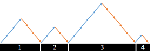
In a grid graph, an isolated path is any maximal sequence of pyramids or valleys all adjoining at the same base level.
A consequence of the definition of an isolated path is it has no st adjoining pyramid or valley. Isolated paths with are isolated pairs. Isolated paths with are isolated quads.
The four boxes in Figure 10 are isolated paths. There are also two pyramid pairs with three peaks in the middle. These pyramids are contained by an exterior pair.
An invocation of Digraph-flat-exact-paths runs iterations from line 4 in Figure 5. One invocation of Digraph-flat-exact-paths converts all of these isolated paths into exact cost edges.


Corollary 3
Given an LDG , where is Dyck (semi-Dyck) and , then one invocation of Digraph-flat-exact-paths finds an exact cost path for an isolated path, where .
Proof: Without loss, the focus is on an isolated path of pyramids. Since the pyramids form an adjoining isolated path, they all have the same base level. This means the pyramids form a flat Dyck path. So an invocation Digraph-flat-exact-paths computes the flat Dyck reachability of all adjoining pyramid pairs by Lemma 9.
A Dyck inner segment is a Dyck word between a set of exterior pairs and , for integers . The word labels a valid Dyck path and is maximal so does not label a valid path containing . The semi-Dyck case has maximal exterior pairs and , for integers . A semi-Dyck inner segment is a semi-Dyck word.
Inner segments are contained by pyramid (valley) bases in the Dyck (semi-Dyck) case. If an inner segment is empty, then the exterior pairs and ( and ) form a pyramid (valley), for .
Corollary 4
Given an LDG , where is Dyck (semi-Dyck) and and , and suppose an cost edge connects an inner segment of exterior pairs. Then one invocation of Digraph-flat-exact-paths finds an exact path through this inner segment and these exterior pairs.
Proof: Suppose a set of exterior pairs contains a cost edge. It must be that, , and by assumption Digraph-flat-exact-paths already found inner segment’s exact cost path by iteration . Thus, Digraph-flat-exact-paths finds the exact cost path including these exterior pairs by Lemma 9.
Consider Digraph-flat-exact-paths. Finding exact cost paths for isolated paths is not compatible with finding paths in their exterior pairs. This incompatibility is handled by careful iterations of Digraph-flat-exact-paths. See a single iteration in Figure 11. When needed, assume lines 3 and 4 are adapted for the Dyck case, see the discussion accompanying Figure 6.
Convention 2 (Atomic invocations of Digraph-flat-exact-paths)
For the worst case of Figure 11, the algorithm Digraph-flat-exact-paths is atomic.
1. G // Fig. 5 (semi-Dyck add Fig. 6) 2. // original edges plus exact paths 3. // AGMY multiplication, extending edges with exact paths 4.
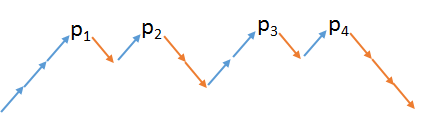
One invocation of Digraph-flat-exact-paths, Figure 5, does not find the exact path from start to end of the top path in Figure 12. Similarly, one invocation of semi-Dyck version of Digraph-flat-exact-paths does not find the exact cost path from start to end for the bottom path.

The next discussion illustrates the challenge of atomic invocations of Digraph-flat-exact-paths. Then we show how iterations of Figure 11 correct for these challenges.
Using label-costs and node names from to , the top path in Figure 12 is,
The Dyck algorithm Digraph-flat-exact-paths fails to find the exact path for . To see this, let be the subpath made of the middle two edges, from node 2 to 4. So, is labeled with and is not Dyck. In its first iteration, the algorithm finds edges and . Also the edges are normalized to edges: and . In the Dyck case, there are no exact paths to extend these new edges, so they are removed in the second iteration. This leaves no exact path from to .
Consider the path at the top of Figure 12. The semi-Dyck version of Digraph-flat-exact-paths finds the exact cost path along . This is because the middle two edges, from node to , are labeled . So in the first iteration, an exact semi-Dyck path is found from to . Also in this iteration, as in the Dyck case, a new is created from to . Likewise, a edge is created from to . All told, in line 9 of the first iteration, the new edge is extended from node to and the edge is extended to go from to . Thus, the second iteration finds the semi-Dyck path from to .
The flat semi-Dyck (Dyck) algorithm Digraph-flat-exact-paths does not find the exact path for the bottom path of Figure 12. This is because in its first iteration it does not find an exact cost path from the first pyramid peak to the fourth pyramid peak. It does find the exact path joining the three exact cost valleys using line 9. This same iteration extends the new edges after normalizing the edges at the start and end. The new edge is extended to the second pyramid peak. The edge is extended from the third pyramid peak. These extensions are all done by line 9. So they are computed in the same algebraic matrix multiplication that forms the exact path joining the three valleys. Therefore, the extended edges cannot reach each other, so in the next iteration they cannot form an exact cost path in line 5.
An iterative solution.
The general solution is based on iterating invocations of Digraph-flat-exact-paths. See Figure 11. After each run of the flat path algorithm, all original edges are extended by the new exact paths. Any new edges are normalized to edges in preparation for the next iteration. The process is repeated for finding more exact paths. After each invocation of Digraph-flat-exact-paths, all new exact paths remain for subsequent iterations.

In Figure 13(a), if the leftmost block is empty, the rightmost block continues recursively using the Figure 13(b), then the leftmost side is an isolated pyramid. In general, if the leftmost (rightmost) block is an isolated path, then it will be replaced by an exact cost path in one invocation of Digraph-flat-exact-paths by Corollary 3. Each time this algorithm find an exact cost path, a new cost edges is created.

This is because, for Dyck paths, Corollary 3 shows pairs of adjoining pyramids require a single invocation of Digraph-flat-exact-paths. Just the same, a single invocation of Digraph-flat-exact-paths also finds an exact path for pyramid pairs. Indeed, reducing adjoining pyramids to pyramids, frees vertices to contribute to worst case subpaths. Similarly, Corollary 4 indicates exterior pairs and , for , may be reduced to exterior pairs and where . Since if and say an exact path is known for an inner segment, then one invocation of Digraph-flat-exact-paths finds the exact path through these exterior pairs. Likewise, a single invocation finds the exact path through exterior pairs and when the exact path is known for the inner segment. So, a reduced worst case Dyck path has all exterior pairs with .
Reduced semi-Dyck paths have exterior pairs and , for . Reduced valleys are labeled . Finally, any pairs of adjoining pyramids and/or valleys are replaced with quads.
Worst case semi-Dyck paths are the exact paths given in Figure 14. If there are only three pyramids in Figure 14(a), then they have two adjoining shared valleys. The first iteration of line 5 creates a edge at the start. Likewise, the first iteration creates a edge at the end. These edges are normalized to new edges in line 7. Finally, line 9 extends the new edges using the two exact paths just made from the two valleys. This gives a edge adjoining a edge for the next iteration. The next iteration of Digraph-flat-exact-paths combines these edges producing an exact path from the start to the end of this path. In summary, semi-Dyck isolated paths with pyramids and/or valleys become exact paths in a single invocation of Digraph-flat-exact-paths.
Definition 12 (Augmented pairs or quads)
A Dyck (semi-Dyck) augmented pair (quad) is a path of two (four) adjoining pyramid (and/or valley) bases whose inner segments are cost edges. All adjoining bases are the same base level and all adjoining bases are contained by an exterior pair.
If two augmented pairs adjoin at the same base level, then these augmented pairs become a single augmented pair in one iteration of Figure 11. Another iteration replaces this single augmented pair with a cost edge. In general, say is a reduced Dyck grid graph with augmented pairs all adjoining at the same base level. If all augmented pairs in have the same maximum level peaks, then all augmented pairs become exact cost paths in the same iteration of Figure 11.
Figure 13 shows how augmented pairs may be constructed. In particular, each level of augmented pairs is contained by an exterior pair. A new augmented pair may only form if this augmented pair has an adjoint augmented pyramid and both together are contained by an exterior pair. The semi-Dyck augmented quads are similar, see Figure 14.

Figure 16 gives reduced Dyck path examples with peaks. In general if is the number of nodes in a reduced Dyck path with peaks, then with the base case . This means , and . Or if , then .
Lemma 10
Consider a reduced Dyck grid path with pyramid peaks and nodes, for an integer . Suppose one pyramid peak is replaced by a cost edge, then Figure 11 requires fewer than iterations to find the exact paths.
Proof: In a grid graph let be a reduced Dyck path with pyramid peaks, for where . These peaks are all at maximum level . Suppose, for the sake of a contradiction, determining that this path is an exact cost path requires iterations.
Since there are pyramid peaks at level , there is at least one pyramid peak that is not in an isolated pair. This single isolated pyramid becomes an exact cost path in the first iteration of Figure 11. So this exact cost path cannot contribute to creating a new augmented pair by an invocation of Digraph-flat-exact-paths. Therefore, at the start of the second iteration of Figure 11, there is an augmented pair that does not have an equivalent neighboring pair to form a new augmented pair. Hence, in the third iteration, there is a new augmented pair just created from two augmented pairs that will not have an equivalent neighboring pair to form a new augmented pair.
In general, the after iterations of this process, there are at least
pyramid peaks that started at the maximum level but they could not form a new augmented pair. This sum is larger than for . For peaks, dropping one peak gives a path with one peak which requires one invocation of the algorithm in Figure 11.
In summary, this means the remaining peaks already formed an exact cost path. Thus, giving a contradiction since iterations are sufficient to find this exact cost path.
In general suppose is the number of nodes in a reduced semi-Dyck path with peaks, for . Therefore, with the base case . This means and . Or if , then , see [42, A007583].
A proof of the next lemma is similar to the proof of Lemma 10.
Lemma 11
Consider a reduced semi-Dyck grid path with pyramids or valleys and nodes, for an integer . Suppose one pyramid or valley is replaced by an exact path, then Figure 11 requires fewer than iterations.
Lemmas 10 and 11 show the worst case Dyck or semi-Dyck paths have maximum peaks at height . Moreover, these results indicate it is sufficient to consider peaks when is a power of 2 for the Dyck case and powers of 4 for the semi-Dyck case.
Lemma 12
Proof: Without loss, consider only reduced Dyck paths.
All Dyck paths are built from pyramids. In reduced paths, all pyramids are in isolated pyramid pairs. The reduced pyramids are . Furthermore, all isolated pyramid pairs have an exterior pair and where .
By Lemma 10, the reduced worst case must start with pyramid peaks, for , at maximum level . The algorithm in Figure 11 finds the exact path in such paths in iterations, since .
A similar argument holds in the semi-Dyck case. The main difference is: semi-Dyck paths are built from pyramids and valleys. Moreover, adjoining isolated paths may be reduced to adjoining elements that are isolated together. Given these differences, all the Dyck arguments just presented remain the same.
This completes the proof.
In the next lemma, height of a grid graph is the value of maximum peak .
Lemma 13
Given an LDG , where is Dyck (semi-Dyck) and , then in the worst case finding all exact paths takes iterations of Figure 11.
Proof: Without loss, the focus is on Dyck paths. Let be the height of a worst-case Dyck path for iterations of the algorithm in Figure 11.
By Lemma 12, the worst-case paths must double their number of isolated pairs at each level. This means after the first iteration, each subsequent iteration of the algorithm in Figure 11 halves the number of augmented pairs.
Therefore, which immediately means . In particular, the additive term of is for each invocation of Digraph-flat-exact-paths.
This section culminates in the main theorem.
Theorem 2
Given an LDG , where is Dyck (semi-Dyck) and , then Figure 11’s algorithm solves Dyck (semi-Dyck) reachability in time.
5 Determining reachability
Determining path reachability in an LDG is based on cost edges computed by the algorithm in Figure 11. After running this algorithm, each cost edge represents an exact cost reachability path. This reachability is either Dyck and semi-Dyck reachability.
Definition 13
Let contain all cost edges found by running the algorithm in Figure 11 times.
The focus is on the edges of in combination with the exact cost edges .
In the case of reachability, consider the next paths from to . Both and are edges in and is an exact cost edge from . So, all cases for and so that are:
If these are the only paths from to , then there is no exact path from to .
Of course, all edges in are built from edges in . An edge is directly from if it is not in an exact cost edge under discussion.
Lemma 14
Given an LDG , its exact cost paths are edges in where is Dyck (semi-Dyck) and , then all paths can be found by extending all edges in with only cost edges in .
Proof: Without loss, the semi-Dyck case is the focus. Recall, semi-Dyck paths are paths with the same number of and edges from .
Consider the edge and another edge in , where ,
so that there is a cost edge from to in .
Let be this cost edge in .
Suppose, for the sake of a contradiction, that ,
is a path that is not discovered by extending with edges from .
Consider the next cases.
Case 1: If and have different signs.
If and have different signs, then the entire path is another cost edge in found by
the algorithm in Figure 11.
This is a contradiction, since in this case joining and does not create a edge.
Case 2: If and have the same sign.
Given the exact edge from between the edges to gives a path: .
Say the path contributes to a edge in combination with another opposite sign edge .
There are two subcases that both lead to contraditions.
-
Subcase 2a: .
This subcase gives which has exact cost . Thus, must be and edge in . Therefore, the reachabilty of requires only to be directly from .
Subcase 2b: .
This subcase gives which also has cost . Thus, must be in . This means the reachabilty of requires only to be directly from .
Since Dyck languages are also semi-Dyck, the proof is complete.
Finding all exact cost edges in an LDG with all edges initially labeled from is the same as determining all reachability in .
Consider the output from Figure 11. Lemma 14 indicates finding all exact cost paths may be computed as the AGMY matrix product,
where is the adjacency matrix of the given LDG . This costs .
6 Conclusion
Acknowledgments
Thanks to Emily Proulx and Sarthak Behl for contributing example inputs and discussing applications of these results.
Thanks to Derek Morris for pointing out interesting applications as well as his encouragement.
References
- [1] P. G. Bradford, “Efficient exact paths for Dyck and semi-Dyck labeled path reachability,” in IEEE 8th Annual Ubiquitous Computing, Electronics Mobile Communication Conference (UEMCON). IEEE Press, 2017, pp. 247–253.
- [2] M. Nykänen and E. Ukkonen, “The exact path length problem,” J. Algorithms, vol. 42, no. 1, pp. 41–53, Jan. 2002.
- [3] L. Lee, “Fast context-free grammar parsing requires fast Boolean matrix multiplication,” Journal of the ACM, vol. 49, no. 1, pp. 1–15, 2002.
- [4] C. Barrett, R. Jacob, and M. Marathe, “Formal language constrained path problems,” SIAM Journal on Computing, vol. 30, no. 3, pp. 809–837, 2001.
- [5] R. Greenlaw, H. J. Hoover, and W. L. Ruzzo, Limits to Parallel Computation: P-Completeness Theory. Oxford University Press, 1995.
- [6] F. Afrati and C. Papadimitriou, “The parallel complexity of simple chain queries,” in Proc. of the 6th ACM Symposium on Principles of Database Systems (PODS ’87). New York, NY, USA: ACM, 1987, pp. 210–213.
- [7] T. Reps, “On the sequential nature of interprocedural program-analysis problems,” Acta Inf., vol. 33, no. 5, pp. 739–757, Aug. 1996. [Online]. Available: http://dx.doi.org/10.1007/BF03036473
- [8] J. D. Ullman and A. Van Gelder, “Parallel complexity of logical query programs,” in 27th Annual Symposium on Foundations of Computer Science, Oct 1986, pp. 438–454.
- [9] M. Yannakakis, “Graph-theoretic methods in database theory,” in PODS ’90: Proceedings of the ninth ACM SIGACT-SIGMOD-SIGART symposium on Principles of database systems. New York, NY, USA: ACM Press, 1990, pp. 230–242.
- [10] D. Coppersmith and S. Winograd, “Matrix multiplication via arithmetic progressions,” Journal of Symbolic Computation, vol. 9, no. 3, pp. 251 – 280, 1990.
- [11] A. J. Stothers, “On the complexity of matrix multiplication,” Ph.D. dissertation, University of Edinburgh, School of Mathematics, 2010.
- [12] V. V. Williams, “Multiplying matrices faster than Coppersmith-Winograd,” in Proceedings of the Forty-fourth Annual ACM Symposium on Theory of Computing, ser. STOC ’12. New York, NY, USA: ACM, 2012, pp. 887–898.
- [13] F. Le Gall, “Powers of tensors and fast matrix multiplication,” in Proceedings of the 39th International Symposium on Symbolic and Algebraic Computation, ser. ISSAC ’14. New York, NY, USA: ACM, 2014, pp. 296–303.
- [14] D. Melski and T. Reps, “Interconvertibility of a class of set constraints and context-free-language reachability,” Theor. Comput. Sci., vol. 248, no. 1-2, pp. 29–98, Oct. 2000.
- [15] N. Alon, Z. Galil, and O. Margalit, “On the exponent of the all pairs shortest path problem,” Journal of Computer and System Sciences, vol. 54, no. 2, pp. 255 – 262, 1997.
- [16] T. Takaoka, “Subcubic cost algorithms for the all pairs shortest path problem,” Algorithmica, vol. 20, no. 3, pp. 309–318, 1998.
- [17] Z. Galil and O. Margalit, “All pairs shortest paths for graphs with small integer length edges,” Journal of Computer and System Sciences, vol. 54, no. 2, pp. 243 – 254, 1997.
- [18] U. Zwick, “All pairs shortest paths using bridging sets and rectangular matrix multiplication,” J. ACM, vol. 49, no. 3, pp. 289–317, May 2002.
- [19] P. G. Bradford and D. A. Thomas, “Labeled shortest paths in digraphs with negative and positive edge weights,” RAIRO - Theoretical Informatics and Applications, vol. 43, no. 3, pp. 567–583, 2009.
- [20] P. G. Bradford, “Quickest path distances on context-free labeled graphs,” in 6th WSEAS Int.Conf. on Info., Security and Privacy (ISP ’07), 2007, pp. 22–29.
- [21] P. G. Bradford and V. Choppella, “Fast point-to-point Dyck constrained shortest paths on a DAG (extended abstract),” in IEEE 7th Annual Ubiquitous Computing, Electronics Mobile Communication Conference (UEMCON). IEEE Press, 2016, pp. 1–7.
- [22] E. Khamespanah, R. Khosravi, and M. Sirjani, “Efficient TCTL model checking algorithm for timed actors,” in Proceedings of the 4th International Workshop on Programming Based on Actors Agents & Decentralized Control, ser. AGERE! ’14. New York, NY, USA: ACM, 2014, pp. 55–66.
- [23] C. B. Ward, N. M. Wiegand, and P. G. Bradford, “A distributed context-free language constrained shortest path algorithm,” in 2008 37th International Conference on Parallel Processing, Sept 2008, pp. 373–380.
- [24] C. B. Ward and N. M. Wiegand, “Complexity results on labeled shortest path problems from wireless routing metrics,” Comput. Netw., vol. 54, no. 2, pp. 208–217, Feb. 2010.
- [25] S. Chaudhuri, “Subcubic algorithms for recursive state machines,” in Proceedings of the 35th Annual ACM SIGPLAN-SIGACT Symposium on Principles of Programming Languages, ser. POPL ’08. New York, NY, USA: ACM, 2008, pp. 159–169.
- [26] W. Rytter, “Fast recognition of pushdown automaton and context-free languages,” Information and Control, vol. 67, no. 1, pp. 12 – 22, 1985.
- [27] H. Yuan and P. Eugster, An Efficient Algorithm for Solving the Dyck-CFL Reachability Problem on Trees. Berlin, Heidelberg: Springer Berlin Heidelberg, 2009, pp. 175–189.
- [28] Q. Zhang, M. R. Lyu, H. Yuan, and Z. Su, “Fast algorithms for dyck-cfl-reachability with applications to alias analysis,” SIGPLAN Not., vol. 48, no. 6, pp. 435–446, Jun. 2013. [Online]. Available: http://doi.acm.org/10.1145/2499370.2462159
- [29] Q. Zhang and Z. Su, “Context-sensitive data-dependence analysis via linear conjunctive language reachability,” SIGPLAN Not., vol. 52, no. 1, pp. 344–358, Jan. 2017. [Online]. Available: http://doi.acm.org/10.1145/3093333.3009848
- [30] N. Hollingum and B. Scholz, Towards a Scalable Framework for Context-Free Language Reachability. Berlin, Heidelberg: Springer Berlin Heidelberg, 2015, pp. 193–211.
- [31] A. Chakrabarti, G. Cormode, R. Kondapally, and A. McGregor, “Information cost tradeoffs for augmented index and streaming language recognition,” SIAM J. Comput., vol. 42, no. 1, pp. 61–83, 2013.
- [32] H. Tang, D. Wang, Y. Xiong, L. Zhang, X. Wang, and L. Zhang, “Conditional dyck-cfl reachability analysis for complete and efficient library summarization,” in Programming Languages and Systems, H. Yang, Ed. Berlin, Heidelberg: Springer Berlin Heidelberg, 2017, pp. 880–908.
- [33] G. Grahne, A. Thomo, and W. W. Wadge, “Preferential regular path queries,” Fundam. Inform., vol. 89, no. 2-3, pp. 259–288, 2008.
- [34] V. Choppella and C. T. Haynes, “Source-tracking unification.” Inf. Comput., vol. 201, no. 2, pp. 121–159, 2005.
- [35] G. Yuval, “An algorithm for finding all shortest paths using infinite-precision multiplications,” Inform. Process. Lett., vol. 4, no. 6, pp. 155–156, 1976.
- [36] T. H. Cormen, C. E. Leiserson, R. L. Rivest, and C. Stein, Introduction to Algorithms (3rd edition). MIT Press, 2009.
- [37] P. W. Purdom, “A transitive closure algorithm,” BIT Numerical Mathematics, vol. 10, no. 1, pp. 76–94, 1970.
- [38] A. V. Aho, J. E. Hopcroft, and J. D. Ullman, The Design and Analysis of Computer Algorithms, 1st ed. Boston, MA, USA: Addison-Wesley Longman Publishing Co., Inc., 1974.
- [39] A. Shoshan and U. Zwick, “All pairs shortest paths in undirected graphs with integer weights,” in IEEE Foundations of Computer Science Conference. IEEE, 1999, pp. 605–615.
- [40] F. Romani, “Shortest-path problem is not harder than matrix multiplication,” Inform. Process. Lett., vol. 11, no. 3, pp. 134 – 136, 1980.
- [41] A. Denise and R. Simion, “Two combinatorial statistics on dyck paths,” Discrete Mathematics, vol. 137, no. 1, pp. 155 – 176, 1995. [Online]. Available: http://www.sciencedirect.com/science/article/pii/0012365X93E0147V
- [42] N. J. A. Sloane (editor). The on-line encyclopedia of integer sequences. Accessed: 2018-02-11. [Online]. Available: https://oeis.org