跳到论文正文
W Papers独立论文阅读器 arXiv:1802.05155 论文正文 计算阅读时间 · 0%
引用这篇论文根据当前论文元数据生成,正式投稿前建议核对。


License: arXiv.org perpetual non-exclusive license
arXiv:1802.05155v5 [cs.LG] 06 Mar 2021

A Diffusion Approximation Theory of Momentum SGD in Nonconvex Optimization

Working in progress.
Tianyi Liu    Zhehui Chen    Enlu Zhou    Tuo Zhao ††thanks: T. Liu, Z. Chen, E. Zhou, and T. Zhao are affiliated with School of Industrial and Systems Engineering at Georgia Tech; Tuo Zhao is the corresponding author; Email: tourzhao@gatech.edu.
Abstract

Momentum Stochastic Gradient Descent (MSGD) algorithm has been widely applied to many nonconvex optimization problems in machine learning, e.g., training deep neural networks, variational Bayesian inference, and etc. Despite its empirical success, there is still a lack of theoretical understanding of convergence properties of MSGD. To fill this gap, we propose to analyze the algorithmic behavior of MSGD by diffusion approximations for nonconvex optimization problems with strict saddle points and isolated local optima. Our study shows that the momentum helps escape from saddle points, but hurts the convergence within the neighborhood of optima (if without the step size annealing or momentum annealing). Our theoretical discovery partially corroborates the empirical success of MSGD in training deep neural networks.

1 Introduction

Nonconvex stochastic optimization naturally arises in many machine learning problems. Taking training deep neural networks as an example, given nn samples denoted by {(xi,yi)}i=1n\{(x_{i},y_{i})\}_{i=1}^{n}, where xix_{i} is the ii-th input feature and yiy_{i} is the response, we solve the following optimization problem,

minθ⁡ℱ⁡(θ):=1n​∑i=1nℓ⁡(yi,f⁡(xi,θ)),\displaystyle\min_{\theta}\mathcal{F}(\theta):=\frac{1}{n}\sumop\displaylimits_{i=1}^{n}\ell(y_{i},f(x_{i},\theta)), (1.1)

where ℓ\ell is a loss function, ff denotes the decision function based on the neural network, and θ\theta denotes the parameter associated with ff. Stochastic Gradient Descent (SGD), which has been known for a long time as stochastic approximation in the control and simulation literature (Robbins and Monro, 1951; Borkar and Meyn, 2000; Kushner and Yin, 2003; Borkar, 2009; Fu et al., 2015), has been applied to solve machine learning problems such as (1.1) (Newton et al., 2018). Momentum Stochastic Gradient Descent (MSGD, Polyak (1964)) is one of the most popular variants of SGD. Specifically, at the tt-th iteration, we uniformly sample ii from (1,…,n)(1,...,n). Then, we take

θ(t+1)=θ(t)−η∇ℓ(yi,f(xi,θ(t)))+μ(θ(t)−θ(t−1)),\displaystyle\theta^{(t+1)}=\theta^{(t)}-\eta\nabla\ell(y_{i},f(x_{i},\theta^{(t)}))+\mu(\theta^{(t)}-\theta^{(t-1)}), (1.2)

where η\eta is the step size parameter and μ∈[0,1)\mu\in[0,1) is the parameter for controlling the momentum. Note that when μ=0\mu=0, (1.2) is reduced to Vanilla Stochastic Gradient Descent (VSGD).

Although SGD-type algorithms have demonstrated significant empirical success for training deep neural networks, their convergence properties for nonconvex optimization are still largely unknown. For VSGD, existing literature (Ghadimi and Lan, 2013) shows that it is guaranteed to converge to a first-order optimal solution (i.e., ∇ℱ​(θ)=0\nabla\mathcal{F}(\theta)=0) under general smooth nonconvex optimization.

The theoretical investigation of MSGD is even more limited than that of VSGD. The momentum in (1.2) has been observed to significantly accelerate computation in practice. To the best of our knowledge, we are only aware of Ghadimi and Lan (2016) in existing literature, which shows that MSGD is guaranteed to converge to a first-order optimal solution for smooth nonconvex problems. Their analysis, however, does not justify the advantage of the momentum in MSGD over VSGD.

To fill the gap between the significant empirical success and the lack of theoretical understanding of MSGD, we are interested in answering a natural and fundamental question in this paper:

What is the role of the momentum in nonconvex stochastic optimization?

The major technical bottleneck in analyzing MSGD and answering the above question comes from the nonconvex optimization landscape of these highly complicated problems, e.g., training large recommendation systems and deep neural networks. We propose to analyze MSGD for nonconvex optimization problems under the assumption of isolated local optima and strict saddle points. This allows us to make progress toward understanding MSGD and gaining new insights on more general problems. Specifically, we consider the following problem:

minx∈Rd⁡ℱ⁡(x)=E⁡[f⁡(x,ξ)],\displaystyle\min_{x\in\mathbb{R}^{d}}\mathcal{F}(x)=\mathbb{E}[f(x,\xi)],

where ξ\xi is a random variable representing the noise, and f⁡(x,ξ)f(x,\xi) is nonconvex in xx given any realization of ξ\xi. We assume that the nonconvex landscape has the following structures: (1) every local optimum has positive curvatures along all directions; (2) there always exist negative curvatures around saddle points (strict saddle property).

The strict saddle property is shared by several popular nonconvex optimization problems arising in machine learning and signal processing, including streaming principle component analysis (PCA), matrix regression/completion/sensing, independent component analysis, partial least square multiview learning, and phase retrieval (Ge et al., 2016; Li et al., 2016; Sun et al., 2016). Moreover, since there is a significant lack of understanding the optimization landscape of general nonconvex problems, many researchers suggest that analyzing strict saddle optimization problems should be considered as the first and important step towards understanding the algorithmic behaviors in general nonconvex optimization. We also want to remark that our analysis can be extended to connected local optima cases. Doing so requires more technical machinery instead of fundamental insights. Therefore, we present the analysis for the isolated optima case for readability and simplicity, and it has already conveyed our core ideas on the effect of momentum.

By making use of the diffusion approximation of stochastic optimization, we provide global and local analysis of MSGD. Specifically, to study the global dynamics, we transfer the discrete time trajectory to a continuous time one by interpolation and prove that asymptotically this continuous time solution trajectory of MSGD converges weakly to the solution of an appropriately constructed ODE. This ODE approximation shows that the momentum helps traverse among stationary points in the non-stationary region, where the variance of the stochastic gradient can be neglected compared with the large magnitude of the gradient. Intuitively, with the help of the momentum, the algorithm makes more progress along the descent direction. Thus, the momentum can accelerate the algorithm in this region by a factor of 11−μ\frac{1}{1-\mu}.

ODE approximation, however, cannot justify how momentum works in the stationary area where the variance of the stochastic gradient dominates the update. To highlight the effect of the variance, we consider the asymptotic behavior of the normalized estimation error obtained by MSGD around the stationary points. We show that the continuous time interpolation of the normalized error sequence converges weakly to a solution of an approximately constructed SDE. By analyzing this SDE solution, we find that the momentum can play different but important roles around saddle points and local optima.

  • •

    The momentum helps escape from the neighborhood of saddle points: In this region, since the gradient diminishes, the variance of the stochastic gradient dominates the algorithmic behavior. Our analysis indicates that the momentum greatly increases the variance and perturbs the algorithm more aggressively. Thus, it becomes harder for the algorithm to stay around saddle points. In addition, the momentum also encourages more aggressive exploitation, and in each iteration, the algorithm makes more progress along the descent direction by a factor of 11−μ\frac{1}{1-\mu}, where μ\mu is the momentum parameter, compared with the VSGD.

  • •

    The momentum hurts the convergence within the neighborhood of local optima: Similar to the neighborhood of saddle points, the gradient dies out, and the variance of the stochastic gradient dominates. Since the momentum increases the variance, it is harder for the algorithm to enter the small neighborhood. To this respect, the momentum hurts in this region. We suggest to apply a step size annealing scheme to neutralize the large variance introduced by momentum within the neighborhood of local optima.

Our ODE/SDE approximation analysis justifies the role of momentum in both stationary and non-stationary areas. However, given the complicated nonconvex landscape, our diffusion approximation analysis cannot establish the second order convergence guarantee and the asymptotic convergence rate of MSGD. Therefore, we further provide a simple but highly non-trival example, streaming PCA, to illustrate our characterization of the effect of momentum and also establish the asymptotic convergence results.

Streaming PCA is a nonconvex problem with only one global optimum and d−1d-1 strict saddle points up to sign change, where dd is the dimension. Its optimization landscape contains the following three regions:

  • •

    𝓡𝟏\bm{\mathcal{R}_{1}}: The region containing the neighborhood of strict saddle points with negative curvatures;

  • •

    𝓡𝟐\bm{\mathcal{R}_{2}}: The region including the set of points whose gradient has sufficiently large magnitude;

  • •

    𝓡𝟑\bm{\mathcal{R}_{3}}: The region containing the neighborhood of all local optima with positive curvatures along all directions.

By studying the corresponding mean ODE and SDE, we show that with arbitrary initialization, MSGD can converge to the global optimum. We provide asymptotic convergence rates of MSGD which precisely quantify the acceleration by momentum in 𝓡𝟏\bm{\mathcal{R}_{1}} and 𝓡𝟐\bm{\mathcal{R}_{2}}. Meanwhile, we also show that with proper step size annealing scheme implemented, MSGD can achieve the same convergence rate as VSGD in 𝓡𝟑.\bm{\mathcal{R}_{3}}.

Our characterization helps explain some phenomena observed when training deep neural networks. There have been some empirical observations and theoretical results (Choromanska et al., 2015) showing that saddle points are the major computation bottleneck, and VSGD usually spends most of the time traveling along saddle and non-stationary regions. Since the momentum helps in both regions, we can find in practice MSGD performs better than VSGD. In addition, from our analysis, the momentum hurts convergence within the neighborhood of the optima. However, we can address this problem by decreasing the step size or the momentum parameter.

We further verify our theoretical findings through numerical experiments on training a residual network (He et al., 2016), using both CIFAR-10 and CIFAR-100 datasets. The experimental results show that the algorithmic behavior of MSGD is consistent with our analysis. Moreover, we observe that with a proper initial step size and a proper step size annealing process, MSGD eventually achieves better generalization accuracy than that of VSGD in training neural networks.

To the best of our knowledge, our proposed theory is the first attempt towards understanding the role of momentum in nonconvex stochastic optimization beyond the convergence to stationary solutions. Taking our results as an initial start, we expect more sophisticated and stronger follow-up work for analyzing momentum SGD, e.g., extending our asymptotic theory to its nonasymptotic counterpart. Please refer to Section 7 for more detailed discussions.

The rest of the paper is organized as follows: Section 2 introduces our nonconvex optimization problem settings and MSGD for solving the problem. Sections 3 and 4 analyze the global and local dynamics of MSGD based on diffusion approximations, respectively; Section 5 studies Streaming PCA and provides an asymptotic convergence rate analysis; Section 6 presents the numerical experiments on both streaming PCA and training deep neural networks to demonstrate our theoretical results; Section 7 makes some further discussions on the related literature, our theoretical and experimental results and future work; The Appendix includes all technical details.

2 Momentum SGD

Recall that we study MSGD for a general nonconvex optimization problem as follows,

minx∈Rd⁡ℱ⁡(x)=E⁡[f⁡(x,ξ)],\displaystyle\min_{x\in\mathbb{R}^{d}}\mathcal{F}(x)=\mathbb{E}[f(x,\xi)], (2.1)

where ξ\xi is a random variable representing the noise and f⁡(x,ξ)f(x,\xi) is nonconvex in xx given any realization of ξ.\xi. We assume that there is a stochastic gradient oracle taking x′∈Rdx^{\prime}\in\mathbb{R}^{d} as input and outputting ∇f​(x′,ξ′),\nabla f(x^{\prime},\xi^{\prime}), where ξ′\xi^{\prime} is a realization of the noise ξ,\xi, such that

E⁡[∇f​(x′,ξ′)]=∇ℱ​(x′),Cov[∇f​(x′,ξ′)]=�.\mathbb{E}[\nabla f(x^{\prime},\xi^{\prime})]=\nabla\mathcal{F}(x^{\prime}),\penalty\ \penalty\ \penalty\ \Cov[\nabla f(x^{\prime},\xi^{\prime})]=\Sigma.

Given a vector v=(v(1),…,v(d))⊤∈Rdv=(v^{(1)},\ldots,v^{(d)})^{\top}\in\mathbb{R}^{d}, we define the vector norm: ‖v‖22=∑j(v(j))2||v||^{2}_{2}=\sumop\displaylimits_{j}(v^{(j)})^{2}. We impose the following standard assumptions on the objective ℱ⁡(x)\mathcal{F}(x) and f⁡(x,ξ).f(x,\xi).

Assumption 1.

  • •

    Uniform Boundedness: There exists a constant CC such that ‖∇f​(x,ξ)‖2≤C,∀x,ξ.||\nabla f(x,\xi)||_{2}\leq C,\penalty\ \penalty\ \forall x,\xi.

  • •

    Lipschitz Continuous: There exists a constant LL such that

    ‖∇ℱ​(x1)−∇ℱ​(x2)‖2≤L​‖x1−x2‖2,∀x1,x2∈Rd.||\nabla\mathcal{F}(x_{1})-\nabla\mathcal{F}(x_{2})||_{2}\leq L||x_{1}-x_{2}||_{2},\quad\forall x_{1},x_{2}\in\mathbb{R}^{d}.

In general, the optimization landscape of (2.1) can be very complicated with numerous local optima and saddle points. Here, we consider the case where all the saddle points satisfy the strict saddle property and every local optimum is isolated as stated in Assumption 2.

Assumption 2 (Isolated Optima and Strict Saddle Points).

Denote S={x∈Rd|∇ℱ​(x)=0}S=\{x\in\mathbb{R}^{d}|\nabla\mathcal{F}(x)=0\} as the set of all stationary points. For x′∈S,x^{\prime}\in S, x′x^{\prime} must be one of the following:

  • •

    A strict saddle point such that λmin​(∇2ℱ​(x′))<0.\lambda_{\min}(\nabla^{2}\mathcal{F}(x^{\prime}))<0.

  • •

    An isolated local optimum such that λmin​(∇2ℱ​(x′))>0.\lambda_{\min}(\nabla^{2}\mathcal{F}(x^{\prime}))>0.

We want to remark that our analysis can also be extended to study the case of connected local optima. However, the proof will be much more involved. Please refer to Section 7 for detailed discussion.

We apply SGD with Polyak’s momentum (Polyak, 1964) (MSGD for short) to solve (2.1). At the kk-th iteration, MSGD takes the following update

xk+1=xk−η∇f(xk,ξk)+μ(xk−xk−1),\displaystyle x_{k+1}=x_{k}-\eta\nabla f(x_{k},\xi_{k})+\mu(x_{k}-x_{k-1}), (2.2)

where η>0\eta>0 is the step size, and μ​(xk−xk−1)\mu(x_{k}-x_{k-1}) is the momentum with the momentum parameter μ∈[0,1)\mu\in[0,1). When μ=0\mu=0, (2.2) is reduced to SGD. We remark that though we focus on Polyak’s momentum, extending our theoretical analysis to Nesterov’s momentum (Nesterov, 1983) is straightforward.

3 Analyzing Global Dynamics by ODE

We first analyze the global dynamics of Momentum SGD (MSGD) by taking a diffusion approximation approach. Roughly speaking, by taking the step size η→0,\eta\rightarrow 0, the continuous-time interpolation of the iterations {xk}k=0∞\{x_{k}\}_{k=0}^{\infty}, which can be treated as a stochastic process with Càdlàg paths (right continuous with left-hand limits), becomes a continuous stochastic process. For MSGD, this continuous process follows an ODE with a unique solution. This ODE helps us understand how the momentum affects the global dynamics. We remark that the momentum parameter μ\mu is a fixed constant in our analysis.

More precisely, we define the continuous-time interpolation Xη​(⋅)X^{\eta}(\cdot) of the solution trajectory of the algorithm as follows: for t≥0t\geq 0, set Xη​(t)=xkηX^{\eta}(t)=x^{\eta}_{k} on the time interval [kη,kη+η).[k\eta,k\eta+\eta). Throughout our analysis, similar notations are applied to other interpolations (e.g. Hη​(t)H^{\eta}(t), Uη​(t)U^{\eta}(t)). We then answer the following question:

Does the solution trajectory sequence {Xη​(⋅)}η\{X^{\eta}(\cdot)\}_{\eta} converge weakly as η\eta goes to zero?
If so, what is the limit?

This question has been studied for VSGD in existing literature for special nonconvex optimization problems, such as streaming PCA in Chen et al. (2017). The Infinitesimal Perturbation Analysis (IPA) technique is widely used to show that under some regularity conditions, Xη​(⋅)X^{\eta}(\cdot) converges weakly to a solution of the following ODE:

X˙​(t)=−∇ℱ​(X​(t)).\dot{X}(t)=-\nabla\mathcal{F}(X(t)). (3.1)

This method, however, cannot be applied to analyze MSGD due to the additional momentum term. Here, we explain why this method fails. Rewrite the algorithm (2.2) as

δk+1=μδk−η∇f(xk,ξk),xk+1=xk+δk+1.\displaystyle\delta_{k+1}=\mu\delta_{k}-\eta\nabla f(x_{k},\xi_{k}),\quad x_{k+1}=x_{k}+\delta_{k+1}.

One can easily check (δk,xk)(\delta_{k},x_{k}) is Markovian. To apply IPA, the Infinitesimal Conditional Expectation (ICE) must converge to a constant. However, the ICE for MSGD, which can be calculated as follows:

E[δk+1−δk|δk,xk]η=(μ−1)​δkη−∇ℱ​(xk),\displaystyle\frac{\mathbb{E}[\delta_{k+1}-\delta_{k}|\delta_{k},x_{k}]}{\eta}=\frac{(\mu-1)\delta_{k}}{\eta}-\nabla\mathcal{F}(x_{k}),

goes to infinity (blows up). Thus, IPA is not applicable here.

To address this challenge, we provide a new technique to prove the weak convergence and find the desired ODE. In a nutshell, we first prove rigorously the weak convergence of the trajectory sequence, and then using martingale theory to find the ODE. For self-containedness, we provide a summary on the pre-requisite weak convergence theory in Appendix A.

Under Assumption 1, we characterize the global behavior of MSGD as follows.

Theorem 3.1.

Let Dd[0,∞)D^{d}[0,\infty) be the space of Rd\mathbb{R}^{d}-valued operators which are right continuous and have left-hand limits for each dimension. Suppose x0=x1∈Rdx_{0}=x_{1}\in\mathbb{R}^{d}. Then for each subsequence of {Xη​(⋅)}η>0\{X^{\eta}(\cdot)\}_{\eta>0}, there exists a further subsequence and a process X⁡(⋅)X(\cdot) such that Xη​(⋅)⇒X​(⋅)X^{\eta}(\cdot)\Rightarrow X(\cdot) in the weak sense as η→0\eta\rightarrow 0 through the convergent subsequence in the space Dd[0,∞)D^{d}[0,\infty), where X⁡(⋅)X(\cdot) satisfies the following ODE:

X˙=−11−μ∇ℱ(X),X(0)=x0.\displaystyle\dot{X}=-\frac{1}{1-\mu}\nabla\mathcal{F}(X),\quad X(0)=x_{0}. (3.2)

Moreover, for any δ>0,\delta>0, there exists a sequence Tη,δ→∞T^{\eta,\delta}\rightarrow\infty such that

lim supη→0P(∃t≤Tη,δ,Xη(t),Nδ(S))=0,\limsup_{\eta\rightarrow 0}\mathbb{P}\left(\exists t\leq T^{\eta,\delta},\penalty\ X^{\eta}(t)\neq N_{\delta}(S)\right)=0,

where Nδ​(S)N_{\delta}(S) is the δ\delta-neighborhood of the stationary points.

Proof Sketch.

To prove this theorem, we first show the trajectory sequence {Xη​(⋅)}η\{X^{\eta}(\cdot)\}_{\eta} converges weakly. By Prokhorov’s Theorem A.3 (in Appendix A), we need to prove tightness, which means {Xη​(⋅)}η\{X^{\eta}(\cdot)\}_{\eta} is bounded in probability in space Dd[0,∞)D^{d}[0,\infty). This can be proved by Theorem A.7 (in Appendix A), which requires the following two conditions: (1) xkx_{k} must be bounded in probability for any kk uniformly in step size η\eta; (2) The maximal discontinuity (the largest difference between two iterations, i.e., maxk⁡{xk+1−xk}\max_{k}\{x_{k+1}-x_{k}\}) must go to zero as η\eta goes to 0.0. This can be shown by using the bounded gradient assumption.

We next compute the weak limit. For simplicity, we define

βkη=−∑i=0k−1μk−i[∇f(xiη,ξi)−∇ℱ(xiη)]andϵkη=−(∇f(xkη,ξk)−∇ℱ(xkη)).\displaystyle\textstyle\beta_{k}^{\eta}=-\sumop\displaylimits_{i=0}^{k-1}\mu^{k-i}[\nabla f(x_{i}^{\eta},\xi_{i})-\nabla\mathcal{F}(x_{i}^{\eta})]\penalty\ \penalty\ \text{and}\penalty\ \penalty\ \epsilon_{k}^{\eta}=-(\nabla f(x_{k}^{\eta},\xi_{k})-\nabla\mathcal{F}(x_{k}^{\eta})).

We then rewrite the algorithm as follows:

mk+1η=mkη+(1−μ)​[−mkη+M~​(xkη)],xk+1η=xkη+η​(mk+1η+βkη+ϵkη),\displaystyle m_{k+1}^{\eta}=m_{k}^{\eta}+(1-\mu)[-m_{k}^{\eta}+\widetilde{M}(x_{k}^{\eta})],\penalty\ \penalty\ x_{k+1}^{\eta}=x_{k}^{\eta}+\eta(m^{\eta}_{k+1}+\beta^{\eta}_{k}+\epsilon^{\eta}_{k}), (3.3)

where M~(x)=−(1−μ)−1∇ℱ(x).\displaystyle\widetilde{M}(x)=-(1-\mu)^{-1}\nabla\mathcal{F}(x). The basic idea of the proof is to view (3.3) as a two-time-scale algorithm (Borkar, 1997; Borkar, 2009), where mkm_{k} is updated with a larger step size (1−μ)(1-\mu) and thus under a faster time-scale, and vkv_{k} is under a slower one. Then we can treat the slower time-scale iterate vv as static and replace the faster time-scale iterate mm by its stable point in term of this fixed vv in (3.3). This stable point can be shown to be M~​(x)\widetilde{M}(x).

We then show that the continuous-time interpolation of the error [mk+1η−M~​(xkη)]+βkη+ϵkη[m^{\eta}_{k+1}-\widetilde{M}(x^{\eta}_{k})]+\beta^{\eta}_{k}+\epsilon^{\eta}_{k} converges weakly to a Lipschitz continuous martingale with zero initialization. From the martingale theory, we know such kind of martingales must be a constant. Thus, the error sequence converges weakly to zero, and what is left is actually the discretization of ODE (3.2). Please refer to Appendix B for the detailed proof. ∎

Note that for any solution X⁡(t)X(t) to (3.1), i.e., the mean ODE of SGD, X⁡(11−μ​t)X(\frac{1}{1-\mu}t) is a solution to (3.2). This implies that asymptotically, MSGD is 11−μ\frac{1}{1-\mu} faster than SGD to converge to the neighborhood of a stationary point given the same initialization. Intuitively, with the help of the momentum, the algorithm makes more progress along the descent direction, and therefore momentum can accelerate the algorithm asymptotically.

However, since the noise of the stochastic gradient diminishes as η→0,\eta\rightarrow 0, such a deterministic ODE-based approach is insufficient to analyze the local behavior of MSGD around stationary points where the noise plays a dominant role over the vanishing gradient. Thus, we resort to the following SDE-based approach for a more precise characterization.

4 Analyzing Local Dynamics by SDE

To characterize the local algorithmic behavior, we need to rescale the influence of the noise. For this purpose, we consider the normalized error xk−x∗η\frac{x_{k}-x^{*}}{\sqrt{\eta}} under the diffusion approximation framework, where x∗∈Sx^{*}\in S is a stationary point. Different from the previous ODE-based approach, we obtain an SDE approximation here. Intuitively, the previous ODE-based approach is analogous to the Law of Large Number for random variables, while the SDE-based approach serves the same role as Central Limit Theorem.

Recall that under Assumption 2, the optimization problem (2.1) has strict saddle points and isolated local optima. We remark that the assumption on isolated local optima helps avoid the cases where the normalization error explodes when the iterate wanders along the connected local optima. Our analysis can be further extended to handle connected local optima. However, the analysis will be much more complicated. Please refer to Section 7 for detailed discussion. For consistency, we first study the algorithmic behavior around the local optimum.

Remark 4.1.

The η\sqrt{\eta} normalization actually normalizes the error by its standard deviation. Specifically, consider the ⌊1/η⌋−\lfloor 1/\eta\rfloor-th iterate of SGD initialized at the stationary point x∗,x^{*},

x⌊1/η⌋=x∗−η​∑i=0⌊1/η⌋−1∇f​(xi)−η​∑i=0⌊1/η⌋−1ξi,x_{\lfloor 1/\eta\rfloor}=x^{*}-\eta\sumop\displaylimits_{i=0}^{\lfloor 1/\eta\rfloor-1}\nabla f(x_{i})-\eta\sumop\displaylimits_{i=0}^{\lfloor 1/\eta\rfloor-1}\xi_{i},

where f⁡(x)f(x) is the objective to be maximized and {ξi}i\{\xi_{i}\}_{i} are the noise in the stochastic gradient i.i.d. sampled from some unknown distribution with mean zero and bounded variance. Given the continuity of the gradient, ∇f​(xi)\nabla f(x_{i}) is approximately zero and noise will dominate around the stationary point x∗.x^{*}. Therefore, x⌊1/η⌋x_{\lfloor 1/\eta\rfloor} can be further approximated as follows.

x⌊1/η⌋≈x∗−η​∑i=0⌊1/η⌋−1ξi.x_{\lfloor 1/\eta\rfloor}\approx x^{*}-\eta\sumop\displaylimits_{i=0}^{\lfloor 1/\eta\rfloor-1}\xi_{i}.

Thus, the variance of the error x⌊1/η⌋−x∗x_{\lfloor 1/\eta\rfloor}-x^{*} is of order O⁡(η)O(\eta):

Var⁡(x⌊1/η⌋−x∗)=η2​Var⁡(∑i=0⌊1/η⌋−1ξi)=O⁡(η).\Var\left(x_{\lfloor 1/\eta\rfloor}-x^{*}\right)=\eta^{2}\Var\left(\sumop\displaylimits_{i=0}^{\lfloor 1/\eta\rfloor-1}\xi_{i}\right)=O(\eta).

Therefore, we actually normalize the error by its standard deviation O⁡(η)O(\sqrt{\eta}), which is analogous to rescaling the sample sum by N\sqrt{N} in Central Limit Theorem.

4.1 Local Dynamics Around Local Optima

We first consider the algorithmic behavior of MSGD when it is around a local optimum x∗x^{*}. Define the normalized process ukη=(xkη−x∗)/η,u_{k}^{\eta}=(x_{k}^{\eta}-x^{*})/\sqrt{\eta}, where λmin​(∇2ℱ​(x∗))>0.\lambda_{\min}(\nabla^{2}\mathcal{F}(x^{*}))>0. Accordingly, Uη​(t)=(Xη​(t)−x∗)/η.U^{\eta}(t)=(X^{\eta}(t)-x^{*})/\sqrt{\eta}. The next theorem characterizes the limiting process of Uη​(t).U^{\eta}(t).

Theorem 4.2.

As η→0\eta\rightarrow 0, {Uη​(⋅)}\{U^{\eta}(\cdot)\} converges weakly to the unique stationary solution of

d​U=−11−μ​∇2ℱ​(x∗)​U​d​t+11−μ​d​Wt,\displaystyle dU=-\frac{1}{1-\mu}\nabla^{2}\mathcal{F}(x^{*})Udt+\frac{1}{1-\mu}dW_{t}, (4.1)

where {Wt}\{W_{t}\} is a Wiener process with covariance matrix �=E[∇f(x∗,ξ)∇f(x∗,ξ)⊤].\Sigma=\mathbb{E}[\nabla f(x^{*},\xi)\nabla f(x^{*},\xi)^{\top}].

Note that our analysis is very different from that in Chen et al. (2017) because of the failure of IPA due to the similar blow-up issue. We remark that our technique mainly relies on Theorem A.8 (in Appendix A) from Kushner and Yin (2003). Since the proof is much more sophisticated and involved than IPA, we introduce the key technique, Fixed-State-Chain, in a high level.

Proof Sketch.

Note that the algorithm can be rewritten as

xk+1η,i\displaystyle x_{k+1}^{\eta,i} =xkη,i−η[∑j=1k−1μk−j∇f(xjη,ξj)+∇ℱ(xk)]−η[∇f(xkη,ξk)−∇ℱ(xkη)].\displaystyle\textstyle=x_{k}^{\eta,i}-\eta\Big[\sumop\displaylimits_{j=1}^{k-1}\mu^{k-j}\nabla f(x_{j}^{\eta},\xi_{j})+\nabla\mathcal{F}(x_{k})\Big]-\eta\left[\nabla f(x_{k}^{\eta},\xi_{k})-\nabla\mathcal{F}(x_{k}^{\eta})\right].

Here, for a vector x∈Rdx\in\mathbb{R}^{d} and an integer i≤di\leq d, x(i)x^{(i)} represents the ii-th dimension of xx. We define

ζkη\displaystyle\zeta^{\eta}_{k} =−[∑j=1k−1μk−j∇f(xjη,ξj)],Zkη=g(ζkη,xkη)+γkη,\displaystyle\textstyle=-\Big[\sumop\displaylimits_{j=1}^{k-1}\mu^{k-j}\nabla f(x_{j}^{\eta},\xi_{j})\Big],\penalty\ \penalty\ Z^{\eta}_{k}=g(\zeta^{\eta}_{k},x^{\eta}_{k})+\gamma_{k}^{\eta},
γkη\displaystyle\gamma_{k}^{\eta} =∇ℱ(xkη)−∇f(xkη,ξk)andg(ζkη,xkη)=ζkη−∇ℱ(xkη).\displaystyle=\nabla\mathcal{F}(x_{k}^{\eta})-\nabla f(x_{k}^{\eta},\xi_{k})\quad\textrm{and}\quad g(\zeta_{k}^{\eta},x_{k}^{\eta})=\zeta_{k}^{\eta}-\nabla\mathcal{F}(x_{k}^{\eta}).

Here, gg is the accelerated gradient flow, and γkη\gamma_{k}^{\eta} is the noise. Then the algorithm becomes

xk+1η=xkη+η​Zkη=xkη+η​g​(ζkη,xkη)+η​γkη,x_{k+1}^{\eta}=x_{k}^{\eta}+\eta Z_{k}^{\eta}=x_{k}^{\eta}+\eta g(\zeta_{k}^{\eta},x_{k}^{\eta})+\eta\gamma_{k}^{\eta},

and thus we have uk+1η=ukη+η​[g⁡(ζkη,xkη)+γkη].u_{k+1}^{\eta}=u_{k}^{\eta}+\sqrt{\eta}[g(\zeta_{k}^{\eta},x_{k}^{\eta})+\gamma_{k}^{\eta}]. Note that g⁡(ζkη,xkη)∈ℱkη​and​E​[γkη|ℱkη]=0g(\zeta_{k}^{\eta},x_{k}^{\eta})\in\mathcal{F}_{k}^{\eta}\penalty\ \textrm{and}\penalty\ \mathbb{E}[\gamma_{k}^{\eta}|\mathcal{F}_{k}^{\eta}]=0 imply that the noise {γkη}\{\gamma_{k}^{\eta}\} is a martingale difference sequence.

We then manipulate the algorithm to extract the Markov structure of the algorithm in an explicit form. To make it clear, given XX, there exists a transition function P(⋅,⋅|X)P(\cdot,\cdot|X) such that

P{ζk+1η∈⋅|ℱkη}=P(ζkη,⋅|X=xkη).P\{\zeta_{k+1}^{\eta}\in\cdot|\mathcal{F}_{k}^{\eta}\}=P(\zeta_{k}^{\eta},\cdot|X=x_{k}^{\eta}).

This comes from the observation ζk+1η=μζkη−μ∇f(xkη,ξkη),\zeta_{k+1}^{\eta}=\mu\zeta_{k}^{\eta}-\mu\nabla f(x_{k}^{\eta},\xi_{k}^{\eta}), where the randomness only comes from ξk\xi_{k} when state xkx_{k} is given. Then the fixed-state-chain refers to the Markov chain with transition function P(⋅,⋅|X)P(\cdot,\cdot|X) for a fixed XX. The state of this Markov chain is denoted by {ζk​(X)}\{\zeta_{k}(X)\}. For notational simplicity, let M~(x)=−11−μ∇ℱ(x).\widetilde{M}(x)=-\frac{1}{1-\mu}\nabla\mathcal{F}(x). We then decompose xk+1η−xkηx_{k+1}^{\eta}-x_{k}^{\eta} as follows:

xk+1η−xkη\displaystyle x_{k+1}^{\eta}-x_{k}^{\eta} =η​M~​(xkη)+η​γkη+η​[g⁡(ζk​(xkη),xkη)−M~​(xkη)]\displaystyle=\eta\widetilde{M}(x_{k}^{\eta})+\eta\gamma_{k}^{\eta}+\eta[g(\zeta_{k}(x_{k}^{\eta}),x_{k}^{\eta})-\widetilde{M}(x_{k}^{\eta})]
+η​[g⁡(ζkη,xkη)−g⁡(ζk​(xkη),xkη)]=η​M~​(xkη)+η​Wkη.\displaystyle\hskip 36.135pt+\eta[g(\zeta_{k}^{\eta},x_{k}^{\eta})-g(\zeta_{k}(x_{k}^{\eta}),x_{k}^{\eta})]=\eta\widetilde{M}(x_{k}^{\eta})+\eta W_{k}^{\eta}. (4.2)

The error term WkηW_{k}^{\eta} in (4.2) comes from three sources: (1) difference between the fixed-state-chain and the limiting process: g⁡(ζk​(xkη),xkη)−M~​(xkη)g(\zeta_{k}(x_{k}^{\eta}),x_{k}^{\eta})-\widetilde{M}(x_{k}^{\eta}); (2) difference between the accelerated gradient flow and the fixed-state-chain: g⁡(ζkη,xkη)−g⁡(ζk​(xkη),xkη)g(\zeta_{k}^{\eta},x_{k}^{\eta})-g(\zeta_{k}(x_{k}^{\eta}),x_{k}^{\eta}); (3) the noise γkη\gamma_{k}^{\eta}.

We handle them separately and combine the results together to get the variance of Wkη,iW_{k}^{\eta,i}. Note that {ukη}\{u_{k}^{\eta}\} satisfies the following update:

uk+1η−ukη=η​M~​(xkη)η+η​Wkη.u_{k+1}^{\eta}-u_{k}^{\eta}=\eta\frac{\widetilde{M}(x_{k}^{\eta})}{\sqrt{\eta}}+\sqrt{\eta}W_{k}^{\eta}.

Together with the fact that around the optimum x∗x^{*}, M~​(x)=−11−μ​∇2ℱ​(x∗)​(x−x∗)+o⁡(‖(x−x∗)‖2),\widetilde{M}(x)=-\frac{1}{1-\mu}\nabla^{2}\mathcal{F}(x^{*})(x-x^{*})+o\left(\|(x-x^{*})\|_{2}\right), we further obtain

uk+1η−ukηη\displaystyle\frac{u_{k+1}^{\eta}-u_{k}^{\eta}}{\eta} =−11−μ​∇2ℱ​(x∗)​ukη+Wkηη+o⁡(|ukη,1|).\displaystyle=-\frac{1}{1-\mu}\nabla^{2}\mathcal{F}(x^{*})u_{k}^{\eta}+\frac{W_{k}^{\eta}}{\sqrt{\eta}}+o\left(|u_{k}^{\eta,1}|\right). (4.3)

After calculating the variance of WW, we see that essentially (4.3) is the discretization of SDE (4.1). For the detailed proof, please refer to Appendix C.1. ∎

Note that (4.1) admits an explicit solution which is known as an Ornstein-Uhlenbeck (O-U) process (Øksendal, 2003) having the following expression:

U⁡(t)=exp⁡(−11−μ​∇2ℱ​(x∗)​t)​U​(0)+∫0texp⁡(11−μ​∇2ℱ​(x∗)​(t−s))​�121−μ​d​Bt.\displaystyle U(t)=\exp\left(-\frac{1}{1-\mu}\nabla^{2}\mathcal{F}(x^{*})t\right)U(0)+\intop\nolimits_{0}^{t}\exp\left(\frac{1}{1-\mu}\nabla^{2}\mathcal{F}(x^{*})(t-s)\right)\frac{\Sigma^{\frac{1}{2}}}{1-\mu}dB_{t}.

Given U⁡(0),U(0), the above formula shows that U⁡(t)U(t) is Gaussian for all t>0.t>0. Therefore, we can identify the limiting density of U⁡(t)U(t) as t→∞t\rightarrow\infty by figuring out the limiting mean and covariance matrix. In fact the mean m⁡(t)=E⁡(U⁡(t))m(t)=\mathbb{E}(U(t)) and covariance matrix ρt=E⁡[U⁡(t)​U​(t)⊤]\rho_{t}=\mathbb{E}[U(t)U(t)^{\top}] satisfy the following ODEs, respectively:

d​m​(t)\displaystyle dm(t) =−∇2ℱ​(x∗)1−μ​m​(t)​d​t,\displaystyle=-\frac{\nabla^{2}\mathcal{F}(x^{*})}{1-\mu}m(t)dt,
d​ρ​(t)\displaystyle d\rho(t) =−11−μ​(∇2ℱ​(x∗)​ρ+ρ​∇2ℱ​(x∗))+1(1−μ)2​�.\displaystyle=-\frac{1}{1-\mu}\left(\nabla^{2}\mathcal{F}(x^{*})\rho+\rho\nabla^{2}\mathcal{F}(x^{*})\right)+\frac{1}{(1-\mu)^{2}}\Sigma.

Since ∇2ℱ​(x∗)\nabla^{2}\mathcal{F}(x^{*}) is positive definite, we have m⁡(t)→0m(t)\rightarrow 0 and

ρμ=limt→∞ρ​(t)=∫0∞exp⁡(−11−μ​∇2ℱ​(x∗)​s)​1(1−μ)2​�​exp⁡(−11−μ​∇2ℱ​(x∗)​s)​𝑑s<∞.\rho_{\mu}=\lim_{t\rightarrow\infty}\rho(t)=\intop\nolimits_{0}^{\infty}\exp\left(-\frac{1}{1-\mu}\nabla^{2}\mathcal{F}(x^{*})s\right)\frac{1}{(1-\mu)^{2}}\Sigma\exp\left(-\frac{1}{1-\mu}\nabla^{2}\mathcal{F}(x^{*})s\right)ds<\infty.

Therefore, when MSGD enters the neighborhood of a local optimum, it will stay near the local optimum and behave like a Brownian motion. Moreover, by a change of variables, we can rewrite ρμ\rho_{\mu} as follows:

ρμ\displaystyle\rho_{\mu} =∫0∞exp⁡(−11−μ​∇2ℱ​(x∗)​s)​1(1−μ)2​�​exp⁡(−11−μ​∇2ℱ​(x∗)​s)​𝑑s\displaystyle=\intop\nolimits_{0}^{\infty}\exp\left(-\frac{1}{1-\mu}\nabla^{2}\mathcal{F}(x^{*})s\right)\frac{1}{(1-\mu)^{2}}\Sigma\exp\left(-\frac{1}{1-\mu}\nabla^{2}\mathcal{F}(x^{*})s\right)ds
=1(1−μ)​∫0∞exp⁡(−∇2ℱ​(x∗)​s)​�​exp⁡(−∇2ℱ​(x∗)​s)​𝑑s\displaystyle=\frac{1}{(1-\mu)}\intop\nolimits_{0}^{\infty}\exp\left(-\nabla^{2}\mathcal{F}(x^{*})s\right)\Sigma\exp\left(-\nabla^{2}\mathcal{F}(x^{*})s\right)ds
=1(1−μ)​ρ0.\displaystyle=\frac{1}{(1-\mu)}\rho_{0}.

We see clearly that the momentum essentially increases the variance of the normalized error by a factor of 11−μ\frac{1}{1-\mu} around the local optimum compared with VSGD. Thus, it becomes harder for the algorithm to converge. The next theorem provides a more precise characterization of such a phenomenon.

Theorem 4.3.

Let (λi,ei)(\lambda_{i},e_{i})’s be the eigenvalue, eigenvector pairs of ∇2ℱ​(x∗)\nabla^{2}\mathcal{F}(x^{*}) such that λ1≥λ2≥…≥λd>0.\lambda_{1}\geq\lambda_{2}\geq...\geq\lambda_{d}>0. Given a sufficiently small ϵ>0\epsilon>0 and ϕ=∑i=1d�i,i<∞\phi=\sumop\displaylimits_{i=1}^{d}\Sigma_{i,i}<\infty, we need the step size η\eta satisfying

η<(1−μ)​λd​ϵ/(4​ϕ)\displaystyle\eta<(1-\mu)\lambda_{d}\epsilon/(4\phi) (4.4)

such that Xη​(t)X^{\eta}(t) enters the ϵ\epsilon-neighborhood of the local optimum with probability at least 3/43/4 at some time T3T_{3} after restarting the counter of time, i.e., ‖Xη​(T3)−x∗‖22≤ϵ,||X^{\eta}(T_{3})-x^{*}||_{2}^{2}\leq\epsilon, where

T3≍(1−μ)2​λd⋅log⁡(8​λd​δ2λd​ϵ−4​η​ϕ),\displaystyle T_{3}\asymp\frac{(1-\mu)}{2\lambda_{d}}\cdot\log\Big(\frac{8\lambda_{d}\delta^{2}}{\lambda_{d}\epsilon-4\eta\phi}\Big),

given ‖Xη​(0)−x∗‖22≤δ2.||X^{\eta}(0)-x^{*}||_{2}^{2}\leq\delta^{2}.

Note that when μ=0,\mu=0, we can choose the step size of VSGD as η0≍λd​ϵ4​ϕ\eta_{0}\asymp\frac{\lambda_{d}\epsilon}{4\phi}, which does not satisfy (4.4) for μ\mu close to 11. This means that when using the same step size of VSGD, MSGD fails to converge, since the variance increased by the momentum becomes too large. To handle this issue, we have to decrease the step size by a factor 1−μ1-\mu, also known as the step size annealing, i.e.,

η≍(1−μ)​ϵ​λd/(4​ϕ)≍(1−μ)​η0.\displaystyle\eta\asymp(1-\mu)\epsilon\lambda_{d}/(4\phi)\asymp(1-\mu)\eta_{0}. (4.5)

We also want to remark that here the probability 3/43/4 can be any constant in (0,1).(0,1). Theorem 4.3 implies the algorithm needs asymptotically at most

N3≍T3η≍ϕϵ​λd2⋅log⁡(8​λd​δ2λd​ϵ−4​η0​ϕ)\displaystyle N_{3}\asymp\frac{T_{3}}{\eta}\asymp\frac{\phi}{\epsilon\lambda_{d}^{2}}\cdot\log\Big(\frac{8\lambda_{d}\delta^{2}}{\lambda_{d}\epsilon-4\eta_{0}\phi}\Big)

iterations to converge to an ϵ\epsilon-optimal solution. Note that the N3N_{3} does not depend on μ\mu. Therefore, MSGD does not have an advantage over VSGD around local optima.

4.2 Local Dynamics Around Saddle Points

We then study the algorithmic behavior around strict saddle points. Define the normalized process ukη=(xkη−x^)/η,u_{k}^{\eta}=(x_{k}^{\eta}-\widehat{x})/\sqrt{\eta}, where x^∈S,λmin​(∇2ℱ​(x^))<0.\widehat{x}\in S,\lambda_{\min}(\nabla^{2}\mathcal{F}(\widehat{x}))<0. Accordingly, Uη​(t)=(Xη​(t)−x^)/η.U^{\eta}(t)=(X^{\eta}(t)-\widehat{x})/\sqrt{\eta}. By the same SDE approximation technique used in Section 4.1, we obtain the following theorem.

Theorem 4.4.

For any C>0,C>0, there exist δ>0\delta>0 and η′>0\eta^{\prime}>0 such that

supη<η′P⁡(supτ>0‖Uη​(τ)‖2≤C)≤1−δ.\displaystyle\sup_{\eta<\eta^{\prime}}\mathbb{P}(\sup_{\tau>0}||U^{\eta}(\tau)||_{2}\leq C)\leq 1-\delta. (4.6)
Proof Sketch.

We prove (4.6) by contradiction. Assume the conclusion does not hold, that is there exists a constant C>0,C>0, such that for any η′>0\eta^{\prime}>0 we have

supη≤η′P⁡(supτ>0|Uη​(τ)|≤C)=1.\sup_{\eta\leq\eta^{\prime}}\mathbb{P}(\sup_{\tau>0}|U^{\eta}(\tau)|\leq C)=1.

That implies there exists a sequence {ηn}n=1∞\{\eta_{n}\}_{n=1}^{\infty} converging to 00 such that

limn→∞P⁡(supτ>0|Uηn​(τ)|≤C)=1.\displaystyle\lim_{n\rightarrow\infty}\mathbb{P}(\sup_{\tau>0}|U^{\eta_{n}}(\tau)|\leq C)=1. (4.7)

We next show that this subsequence {Uηn​(⋅)}n\{U^{\eta_{n}}(\cdot)\}_{n} is tight. To do so, we need to verify two conditions of Theorem A.6 in Appendix A. By (4.7), we know that condition (i) in Theorem A.6 holds. We next check condition(ii) in Theorem A.6. When supτ>0|Uηn,i​(τ)|≤C\sup_{\tau>0}|U^{\eta_{n},i}(\tau)|\leq C holds, Assumption 1 yields that ‖uk+1ηn−ukηn‖2≤C′​ηn,||u_{k+1}^{\eta_{n}}-u_{k}^{\eta_{n}}||_{2}\leq C^{\prime}\eta_{n}, where C′C^{\prime} is some constant. Thus, for any t,ϵ>0,t,\epsilon>0, we have

‖Uηn​(t)−Uηn​(t+ϵ)‖2≤ϵ/η​C′​η=C′​ϵ,\|U^{\eta_{n}}(t)-U^{\eta_{n}}(t+\epsilon)\|_{2}\leq\epsilon/\eta C^{\prime}\eta=C^{\prime}\epsilon,

or equivalently

ϖT′​(Uηn,ϵ)≤C′​ϵ,∀T>0,\varpi^{\prime}_{T}(U^{\eta_{n}},\epsilon)\leq C^{\prime}\epsilon,\forall T>0,

where ϖ\varpi is the modulus of continuous defined in Definition A.5. Thus, condition (ii) in Theorem A.6 holds. Then we have {Uηn​(⋅)}n\{U^{\eta_{n}}(\cdot)\}_{n} is tight and thus converges weakly. Following similar lines to Theorem 4.2, we can verify C.5-C.8 and show that {Uηn​(⋅)}n\{U^{\eta_{n}}(\cdot)\}_{n} converges weakly to a solution of

d​U=−11−μ​∇2ℱ​(x^)​U​d​t+11−μ​d​Wt.\displaystyle dU=-\frac{1}{1-\mu}\nabla^{2}\mathcal{F}(\widehat{x})Udt+\frac{1}{1-\mu}dW_{t}. (4.8)

The process defined by (4.8) is an unstable O-U process. When initialized at x^,\widehat{x}, it has mean 00 and exploding variance. When not initialized at x^,\widehat{x}, it has exploding mean and variance. Thus, for any δ,\delta, there exist a time τ′\tau^{\prime}, such that

P⁡(‖U⁡(τ′)‖1≥C)≥2​δ.\mathbb{P}(\|U(\tau^{\prime})\|_{1}\geq C)\geq 2\delta.

Since {Uηn}n\{U^{\eta_{n}}\}_{n} converges weakly to U,U, {Uηn​(τ′)}n\{U^{\eta_{n}}(\tau^{\prime})\}_{n} converges in distribution to U⁡(τ′).U(\tau^{\prime}). This implies that there exists N>0N>0, such that for any n>N,n>N,

|P⁡(‖U⁡(T)‖2≥C)−P⁡(‖Uηn​(T)‖2≥C)|≤δ.|{\mathbb{P}(\|U(T)\|_{2}\geq C)-\mathbb{P}(\|U^{\eta_{n}}(T)\|_{2}\geq C)}|\leq{\delta}.

Then we find a τ′>0\tau^{\prime}>0 such that

P⁡(‖Uηn​(τ′)‖2≥C)≥δ,∀n>N,\mathbb{P}(\|U^{\eta_{n}}(\tau^{\prime})\|_{2}\geq C)\geq{\delta},\quad\forall n>N,

or equivalently

P⁡(‖Uηn​(τ′)‖2≤C)<1−δ,∀n>N.\mathbb{P}(\|U^{\eta_{n}}(\tau^{\prime})\|_{2}\leq C)<1-{\delta},\quad\forall n>N.

Since {ω|supτ‖Uηn​(τ)​(ω)‖2≤C}⊂{ω|‖Uηn​(τ′)​(ω)‖2<C},\left\{\omega\big|\sup_{\tau}\|U^{\eta_{n}}(\tau)(\omega)\|_{2}\leq C\right\}\subset\left\{\omega\big|\|U^{\eta_{n}}(\tau^{\prime})(\omega)\|_{2}<C\right\}, we have

P⁡(supτ‖Uηn​(τ)‖2≤C)≤1−δ,∀n>N,\mathbb{P}(\sup_{\tau}\|U^{\eta_{n}}(\tau)\|_{2}\leq C)\leq 1-{\delta},\quad\forall n>N,

which leads to a contradiction with (4.7). Our assumption does not hold. We prove Theorem 4.4. ∎

Theorem 4.4 implies that with a constant probability δ,\delta, MSGD escapes from the saddle points at some time T1T_{1}, i.e., ‖Xη​(T1)−x^‖22||X^{\eta}(T_{1})-\widehat{x}||_{2}^{2} is greater than δ2\delta^{2} (δ=𝒪⁡(η)\delta=\mathcal{O}(\sqrt{\eta})). Note that from the proof of Theorem 4.4, when the step size η\eta is small, the process defined by SDE (4.8) characterizes the local behavior of XηX^{\eta} around saddle points. For any fixed μ,\mu, let UμU_{\mu} be the solution to (4.8). Then we can verify that

E⁡(Uμ​(t))=11−μ​E​(U0​(t)),Var⁡(Uμ​(t))=11−μ​Var⁡(U0​(t)).\displaystyle\mathbb{E}(U_{\mu}(t))=\frac{1}{1-\mu}\mathbb{E}(U_{0}(t)),\penalty\ \penalty\ \penalty\ \Var(U_{\mu}(t))=\frac{1}{1-\mu}\Var(U_{0}(t)).

More precisely, we can obtain the following proposition on the asymptotic escaping rate of MSGD.

Theorem 4.5.

Let ∇2ℱ​(x^)=P​�​P⊤\nabla^{2}\mathcal{F}(\widehat{x})=P\Lambda P^{\top} be the eigenvalue decomposition of ∇2ℱ​(x^),\nabla^{2}\mathcal{F}(\widehat{x}), where �=diag⁡(λ1,…,λd)\Lambda={\rm diag}(\lambda_{1},...,\lambda_{d}) and λ1≥λ2≥…≥λd\lambda_{1}\geq\lambda_{2}\geq...\geq\lambda_{d} and λd<0.\lambda_{d}<0. Denote �=E[∇f(x^,ξ)∇f(x^,ξ)⊤].\Sigma=\mathbb{E}[\nabla f(\widehat{x},\xi)\nabla f(\widehat{x},\xi)^{\top}]. Given a pre-specified ν∈(0,1)\nu\in(0,1), η≍η0\eta\asymp\eta_{0}, and δ=𝒪⁡(η)\delta=\mathcal{O}(\sqrt{\eta}), then the following result holds: We need at most

T1≍(1−μ)2​|λd|​log⁡(2​η−1​δ2​(1−μ)​|λd|�−1​(916)2​(P⊤​�​P)d,d+1),\displaystyle T_{1}\asymp\frac{(1-\mu)}{2|\lambda_{d}|}\log\left(\frac{2\eta^{-1}\delta^{2}(1-\mu)|\lambda_{d}|}{\Phi^{-1}\left(\frac{9}{16}\right)^{2}(P^{\top}\Sigma P)_{d,d}}+1\right), (4.9)

such that ‖Xη​(T1)−x^‖22≥δ2\displaystyle||X_{\eta}(T_{1})-\widehat{x}||_{2}^{2}\geq\delta^{2} with probability at least 34\frac{3}{4}, where �⁡(x)\Phi(x) is the CDF of the standard normal distribution.

Theorem 4.5 suggests that we need asymptotically

N1≍(1−μ)​ϕ|λd|2​ϵ​log⁡(2​(1−μ)​η−1​δ2​|λd|�−1​(1+ν/22)2​(P⊤​�​P)d,d+1)\displaystyle N_{1}\asymp\frac{(1-\mu)\phi}{|\lambda_{d}|^{2}\epsilon}\log\left(\frac{2(1-\mu)\eta^{-1}\delta^{2}|\lambda_{d}|}{\Phi^{-1}\left(\frac{1+\nu/2}{2}\right)^{2}(P^{\top}\Sigma P)_{d,d}}+1\right)

iterations to escape from saddle points. Thus, when using the same step size, MSGD can escape from saddle points in fewer iterations than VSGD by a factor of 1−μ1-\mu. This is due to the fact that the momentum can greatly increase the variance and perturb the algorithm more aggressively. Thus, it becomes harder to stay around saddle points. Moreover, the momentum also encourages more aggressive exploitation, and in each iteration, the algorithm makes more progress along the descent direction by a factor of 11−μ\frac{1}{1-\mu}.

In summary, compared with VSGD (μ=0\mu=0), momentum accelerates escaping from saddle points by a factor of 1−μ.1-\mu. However, momentum can also hurt the final convergence around the local optimum because of the increased variance. Therefore, we suggest to decrease the step size by a factor 1−μ1-\mu in the later stage, MSGD can then achieve the similar convergence rate as VSGD. Note that we can also decrease the momentum parameter μ\mu instead of the step size η.\eta. We will show in Section 6 that momentum annealing and step size annealing can both ensure the convergence of MSGD.

5 Example: Streaming PCA

In this section, we apply our convergence analysis to study the algorithmic behavior of MSGD and provide explicit convergence result for the streaming PCA problem formulated as follows.

maxv⁡v⊤​EX∼𝒟​[X​X⊤]​vsubject tov∈S={v∈Rd|‖v‖2=1}.\displaystyle\max_{v}\;v^{\top}\mathbb{E}_{X\sim\mathcal{D}}[XX^{\top}]v\quad\textrm{subject to}\penalty\ \penalty\ v\in\mathbb{S}=\{v\in\mathbb{R}^{d}\,|\,\|v\|_{2}=1\}. (5.1)

For notational simplicity, we denote the covariance matrix as �=E⁡[X​X⊤]\Sigma=\mathbb{E}[XX^{\top}] . Before we proceed, we impose the following assumption on �\Sigma:

Assumption 3.

The covariance matrix �\Sigma is positive definite with eigenvalues λ1>λ2≥…≥λd>0\lambda_{1}>\lambda_{2}\geq...\geq\lambda_{d}>0 and associated normalized eigenvectors v1,v2,…,vdv^{1},\,v^{2},\,...,\,v^{d}. Moreover, there exists an orthogonal matrix Q such that: �=Q​�​Q⊤,\Sigma=Q\Lambda Q^{\top}, where �=diag⁡(λ1,λ2,…,λd).\Lambda={\rm diag}(\lambda_{1},\lambda_{2},...,\lambda_{d}).

Under this assumption, the optimization landscape of (5.1) has been well studied. Chen et al. (2017) have shown that the eigenvectors ±v1,±v2,…,±vd\pm v^{1},\,\pm v^{2},\,...,\,\pm v^{d} are all the stationary points for problem (5.1) on the unit sphere S\mathbb{S}. Moreover, the eigen-gap assumption (λ1>λ2\lambda_{1}>\lambda_{2}) guarantees that the global optimum v1v^{1} is identifiable up to sign change. Meanwhile, v2,…,vd−1v^{2},\,...,\,v^{d-1} are d−2d-2 strict saddle points, and vdv^{d} is the global minimum.

Given the optimization landscape of (5.1), we have already understood well the behavior of VSGD algorithms, including Oja’s rule and stochastic generalized Hebbian algorithms (SGHA) for streaming PCA (Chen et al., 2017). We consider a variant of SGHA with Polyak’s momentum (Polyak, 1964). Recall that we are given a streaming data set {Xk}k=1∞\{X_{k}\}_{k=1}^{\infty} drawn independently from some zero-mean distribution 𝒟\mathcal{D}. At the kk-th iteration, the algorithm takes

vk+1=vk+η​(I−vk​vk⊤)​�k​vk+μ​(vk−vk−1),\displaystyle v_{k+1}=v_{k}+\eta(I-v_{k}v_{k}^{\top})\Sigma_{k}v_{k}+\mu(v_{k}-v_{k-1}), (5.2)

where �k=Xk​Xk⊤\Sigma_{k}=X_{k}X_{k}^{\top} and μ​(vk−vk−1)\mu(v_{k}-v_{k-1}) is the momentum with a parameter μ∈[0,1)\mu\in[0,1). When μ=0\mu=0, (5.2) is reduced to SGHA. A detailed derivation of (5.2) is provided in Appendix D.

Remark 5.1.

The constraint in problem (5.1) restricts the solution space to be a unit sphere S,\mathbb{S}, which is a manifold. In order to match our algorithm (1.2), we consider (5.1) to be an unconstraint optimization problem on the manifold by using the manifold gradient (I−x​x⊤)​�​x(I-xx^{\top})\Sigma x. For general manifold optimization problems, additional projection may be required to ensure the solution trajectory staying on the manifold. However, for the sphere constraint as in (5.1), when η\eta is small, moving along the direction of the manifold gradient, the solution trajectory can stay close to S,\mathbb{S}, as shown in Lemma D.1 in Appendix D.

Before we proceed, we impose the following assumption on the problem:

Assumption 4.

The data points {Xk}k=1∞\{X_{k}\}_{k=1}^{\infty} are drawn independently from a distribution 𝒟\mathcal{D} in RdR^{d}, such that:

E⁡[X]=0,E⁡[X​X⊤]=�,‖X‖≤Cd,\mathbb{E}[X]=0,\penalty\ \mathbb{E}[XX^{\top}]=\Sigma,\penalty\ \|X\|\leq C_{d},

where CdC_{d} is a constant (possibly dependent on dd).

This uniformly boundedness assumption can actually be relaxed to the boundedness of the (4+δ)(4+\delta)-th-order moment (δ>0\delta>0) with a careful truncation argument. The proof, however, will be much more involved and beyond the scope of this paper. Thus, we use the uniformly boundedness assumption for convenience.

Under Assumptions 3 and 4, we first apply Theorem 3.1 and provide an ODE approximation for Algorithm (5.2) in the following corollary.

Corollary 5.2.

Suppose v0=v1∈Sv_{0}=v_{1}\in\mathbb{S}. Then Vη​(⋅)⇒V​(⋅)V^{\eta}(\cdot)\Rightarrow V(\cdot) in the weak sense as η→0\eta\rightarrow 0 in the space Dd[0,∞)D^{d}[0,\infty), where V⁡(⋅)V(\cdot) is the unique solution to the following ODE:

V˙=11−μ​(�​V−V⊤​�​V​V),V⁡(0)=v0,\dot{V}=\frac{1}{1-\mu}(\Sigma V-V^{\top}\Sigma VV),\penalty\ \penalty\ V(0)=v_{0}, (5.3)

and has the following explicit form V⁡(t)=Q​H​(t),V(t)=QH(t), where

H(i)(t)=(∑i=1d[H(i)(0)exp(λi​t1−μ)]2)−12H(i)(0)exp(λi​t1−μ),i=1,…,d,H^{(i)}(t)=\Big(\sumop\displaylimits_{i=1}^{d}[H^{(i)}(0)\exp\Big(\frac{\lambda_{i}t}{1-\mu}\Big)]^{2}\Big)^{-\frac{1}{2}}H^{(i)}(0)\exp\left(\frac{\lambda_{i}t}{1-\mu}\right),\quad i=1,...,d,

where H⁡(0)=Q⊤​v0.H(0)=Q^{\top}v_{0}. Moreover, suppose v0,±vi,∀i=2,…,d,v_{0}\neq\pm v^{i},\penalty\ \forall i=2,...,d, as t→∞,t\rightarrow\infty, V⁡(t)V(t) converges to v1,v^{1}, which is the global maximum to (5.1).

Please refer to Appendix D.3 for the detailed proof. Different from the general ODE (3.2), ODE (5.3) has an explicit form solution which implies that whenever MSGD escapes from strict saddle points vi,i≥2v^{i},\penalty\ i\geq 2, it will directly converge to the global optimum v1.v^{1}. Therefore, we can provide a more precise characterization of the algorithmic behavior in the non-stationary area for streaming PCA than general nonconvex problems. Moreover, since streaming PCA has one isolated global optimum and strict saddle points, our SDE analysis for the stationary area can be directly applied. We have the following corollary to characterize the asymptotic convergence rate of MSGD.

Corollary 5.3.

Let η\eta be the step size of MSGD and η0≍(λ1−λ2)​ϵϕ\eta_{0}\asymp\frac{(\lambda_{1}-\lambda_{2})\epsilon}{\phi} be the step size of VSGD as chosen in Chen et al. (2017).

∙\bullet Phase I: Escape from Saddle Points. Suppose v0η=v2,v^{\eta}_{0}=v^{2}, the strict saddle point corresponding to λ2.\lambda_{2}. Given η≍η0\eta\asymp\eta_{0}, and δ=𝒪⁡(η)\delta=\mathcal{O}(\sqrt{\eta}), we need asymptotically at most

N1≍(1−μ)​ϕ(λ1−λ2)2​ϵ​log⁡(2​(1−μ)​η−1​δ2​(λ1−λ2)�−1​(916)2​α122+1),\displaystyle N_{1}\asymp\frac{(1-\mu)\phi}{(\lambda_{1}-\lambda_{2})^{2}\epsilon}\log\left(\frac{2(1-\mu)\eta^{-1}\delta^{2}(\lambda_{1}-\lambda_{2})}{\Phi^{-1}\left(\frac{9}{16}\right)^{2}\alpha^{2}_{12}}+1\right), (5.4)

iterations such that ‖vN1η−v2‖22≥δ2\displaystyle||v^{\eta}_{N_{1}}-v_{2}||_{2}^{2}\geq\delta^{2} with probability at least 3/43/4, where �⁡(x)\Phi(x) is the CDF of the standard normal distribution.

∙\bullet Phase II: Traverse from Saddle Points to the Global Optimum. Suppose ‖v0η−vi‖22≥δ2,∀i≥2.||v^{\eta}_{0}-v^{i}||_{2}^{2}\geq\delta^{2},\penalty\ \penalty\ \forall i\geq 2. For sufficiently small η\eta, δ=𝒪⁡(η)\delta=\mathcal{O}(\sqrt{\eta}), we need

N2≍(1−μ)​ϕ2​ϵ​(λ1−λ2)2​log⁡(2−δ2δ2)\displaystyle N_{2}\asymp\frac{(1-\mu)\phi}{2\epsilon(\lambda_{1}-\lambda_{2})^{2}}\log\left(\frac{2-\delta^{2}}{\delta^{2}}\right) (5.5)

iterations such that ‖vN2η−v1‖22≤δ2\left\|v^{\eta}_{N_{2}}-v^{1}\right\|_{2}^{2}\leq\delta^{2} with probability at least 3/4.{3}/{4}.

∙\bullet Phase III: Converge to the Global Optimum. For a sufficiently small ϵ>0\epsilon>0 and η≍(1−μ)​η0\eta\asymp(1-\mu)\eta_{0}, there exists some constant δ=𝒪⁡(η)\delta=\mathcal{O}(\sqrt{\eta}), such that ‖v0η−v1‖2≤δ2\left\|v^{\eta}_{0}-v^{1}\right\|^{2}\leq\delta^{2}, we need

N3≍ϕϵ​(λ1−λ2)2⋅log⁡(8​(λ1−λ2)​δ2(λ1−λ2)​ϵ−4​η0​ϕ)\displaystyle N_{3}\asymp\frac{\phi}{\epsilon(\lambda_{1}-\lambda_{2})^{2}}\cdot\log\Big(\frac{8(\lambda_{1}-\lambda_{2})\delta^{2}}{(\lambda_{1}-\lambda_{2})\epsilon-4\eta_{0}\phi}\Big) (5.6)

iterations to ensure ‖vN3η−v1‖22≤ϵ\left\|v^{\eta}_{N_{3}}-v^{1}\right\|_{2}^{2}\leq\epsilon with probability at least 3/43/4 .

Please refer to Appendix D.4 for the detailed proof. From Corollary 5.3, we can see clearly that momentum accelerates escaping from saddle points and traversal to the global optimum by a factor of 1−μ.1-\mu. If we further decrease the step size in Phase III, MSGD can achieve the same convergence rate as VSGD.

6 Numerical Experiments

We present numerical experiments for both streaming PCA and training deep neural networks. The experiments on streaming PCA verify our theory in Section 5, and the experiments on training deep neural networks support our theoretical results for the general problem and also verify some of our discussions in Section 7 later.

6.1 Streaming PCA

We first provide a numerical experiment to verify our theory for streaming PCA. We set d=4d=4 and the covariance matrix �=diag​{4,3,2,1}.\Lambda=\rm{diag}\{4,3,2,1\}. The optimum is (1,0,0,0).(1,0,0,0). Figure 1 compares the performance of VSGD, MSGD (with and without the step size annealing, and momentum annealing in Phase III). The initial solution is the saddle point (0,1,0,0)(0,1,0,0). We choose μ=0.9\mu=0.9 and η=5×10⁻⁴\eta=5\times 10^{-4}, decrease the step size of MSGD by a factor 1−μ1-\mu after 2×1042\times 10^{4} iterations in Figure 1.b, and decrease the momentum by a factor 1/101/10 after 2×1042\times 10^{4} iterations in Figure 1.c. Figure 1 plot the results of 100 simulations, and the vertical axis corresponds to ||Hk(1)|−1|||H_{k}^{(1)}|-1|. We can clearly differentiate the three phases of VSGD in Figure 1.a. For MSGD in Figures 1.b, 1.c and 1.d, we hardly recognize Phases I and II, since they last for a much shorter time. This is because the momentum significantly helps escape from saddle points and evolve toward the global optimum. Moreover, we also observe in Figure 1.b that MSGD without the step size annealing and the momentum annealing does not converge well, but the step size annealing or the momentum annealing resolves this issue. All these observations are consistent with our analysis. Figure 1.e plots the optimization errors of these three algorithms averaged over all 100 simulations, and we observe similar results.

Refer to caption
(a) Three phases in SGD.
Refer to caption
(b) MSGD does not converge.
Refer to caption
(c) MSGD with SSA converges.
Refer to caption
(d) MSGD with MA converges.
Refer to caption
(e) Comparison among SGD and different MSGDs.
Figure 1: Comparison between SGD and MSGD (with and without the Step Size Annealing (SSA) and Momentum Annealing (MA) in Phase III).

6.2 Deep Neural Networks

Momentum SGD and its variants has been widely applied in training deep neural networks (Sutskever et al., 2013; Kingma and Ba, 2014; Goodfellow et al., 2016; He et al., 2016) and has been implemented in popular deep learning libraries, such as Tensorflow (Abadi et al., 2016) and PyTorch (Paszke et al., 2019). In this section, we present several experiments to compare MSGD with VSGD in training a 9-layer Residual Net (ResNet-9, Page (2018)) over CIFAR-1010 and CIFAR-100100 datasets for 1010 and 100100-class image classification tasks, respectively. Both datasets contain 6060k images, in which 5050k images are used for training, and the rest 1010k are used for testing. The network architecture of ResNet-9 is shown in Figure 2 and summarized in Table 1. All experiments are done in PyTorch with one NVIDIA RTX 2080-Ti GPU. For each experiment, we repeat for 2020 times with different random seeds and report the average and standard deviation.

(a) An illustrative visualization of 9 layers in ResNet-9 (ResBlock contains 2 layers)
(b) Grey convolutional layer
(c) Pink convolutional layer
(d) Residual block: containing two convolutional layers
Figure 2: The Network Architecture of ResNet-9 and Its Detailed Components.
Table 1: Network Architecture of ResNet-9.
Layer Output size Filter, activation and pooling
Conv 32×3232\times 32 [3×3,64]×1[3\times 3,64]\times 1, stride 1
Conv 16×1616\times 16 [3×3,128]×1[3\times 3,128]\times 1, stride 1, Max pooling (2)
Residual Block 16×1616\times 16 [3×3,128][3\times 3,128], stride 1
Conv 8×88\times 8 [3×3,216]×1[3\times 3,216]\times 1, stride 1, Max pooling (2)
Conv 4×44\times 4 [3×3,512]×1[3\times 3,512]\times 1, stride 1, Max pooling (2)
Residual Block 4×44\times 4 [3×3,512][3\times 3,512], stride 1
Linear Number of classes Max pooling (4), fully connected

We adopt the training configure from Page (2018), which uses the label smooth loss function (Szegedy et al., 2016). Specifically, for a KK classification problem, given a training sample xx with class yy, we denote its predicted probability for class ii as pi​(x)p_{i}(x), and then the loss function is

f⁡(x,y,ϵ)=(1−ϵ)​∑i=1Kδi​(y)​log⁡pi​(x)+ϵK​∑i=1Klog⁡pi​(x),\displaystyle f(x,y;\epsilon)=(1-\epsilon)\sumop\displaylimits_{i=1}^{K}\delta_{i}(y)\log p_{i}(x)+\frac{\epsilon}{K}\sumop\displaylimits_{i=1}^{K}\log p_{i}(x),

where ϵ\epsilon denotes the smoothing parameter, and δi(y)=𝟏{i=y}\delta_{i}(y)=\mathbf{1}_{\{i=y\}} is the indicator function. In our experiments, we set ϵ\epsilon as 0.20.2. In addition, for each experiment, we train the network for 100100 epochs and use the batch size as 512512. Moreover, we use the state-of-the-art step size setting with warmup as follows:

ηi={i20​η,1≤i≤20,(1−i−2080)​η,21≤i≤100,\eta_{i}=\begin{cases}\frac{i}{20}\eta,&1\leq i\leq 20,\\ \left(1-\frac{i-20}{80}\right)\eta,&21\leq i\leq 100,\end{cases}

where ηi\eta_{i} is the step size used in the ii-th epoch for 1≤i≤100.1\leq i\leq 100. The warmup is effective to obtain a good parameter in training deep neural network.

For MSGD, we set the momentum parameter μ\mu as 0.90.9, and choose the step size ηM\eta_{\textrm{M}} as {0.04ℓ:ℓ∈N,4≤ℓ≤15}.\{0.04\ell:\ell\in\mathbb{N},4\leq\ell\leq 15\}. Thus, for VSGD, we use the equivalent step size of MSGD (ηV=ηM1−μ\eta_{\mathrm{V}}=\frac{\eta_{\mathrm{M}}}{1-\mu}) chosen from {0.4ℓ:ℓ∈N,4≤ℓ≤15}.\{0.4\ell:\ell\in\mathbb{N},4\leq\ell\leq 15\}. Figures 3 and 4 show that the comparisons of loss values between the MSGD and the VSGD with their best settings over CIFAR-10. As can be seen, the validate loss of MSGD decreases faster than that of the VSGD and eventually achieves a smaller value. For more comparison results, please see Appendix E. In addition, Table 2 presents the validate accuracy of both MSGD and VSGD over CIFAR datasets. As can be seen, in average, the MSGD is better than the VSGD with the equivalent step size over CIFAR-10 and CIFAR-100 tasks. We further test the significance of the pairwise comparison between the best MSGD and the best VSGD. For CIFAR-10 (ηM=0.36\eta_{\mathrm{M}}=0.36 and ηV=2\eta_{\mathrm{V}}=2) and CIFAR-100 (ηM=0.56\eta_{\mathrm{M}}=0.56 and ηV=2.4\eta_{\mathrm{V}}=2.4), the corresponding pp-values are 0.0108\mathbf{0.0108} and 1.023×𝟏𝟎−𝟓\mathbf{1.023\times 10^{-5}}, respectively. This shows that the best MSGD significantly outperforms the best VSGD.

(a) Best setting: ηV=2\eta_{\textrm{V}}=2 and ηM=0.36\eta_{\textrm{M}}=0.36
(b) Zoom-in for the best setting
Figure 3: Experimental Results of ResNet-9 on CIFAR-10 under the Best Settings: 𝜼V=𝟐\bm{\eta_{\textrm{V}}=2}, 𝜼M=0.36\bm{\eta_{\textrm{M}}=0.36}.
(a) Best setting: ηV=2.4\eta_{\textrm{V}}=2.4 and ηM=0.56\eta_{\textrm{M}}=0.56
(b) Zoom-in for the best setting
Figure 4: Experimental Results of ResNet-9 on CIFAR-100 under the Best Ssettings: 𝜼V=2.4\bm{\eta_{\textrm{V}}=2.4}, 𝜼M=0.56\bm{\eta_{\textrm{M}}=0.56}.
Table 2: Results of Validation Accuracy and the Corresponding Standard Deviations (in the Bracket) for the Last Epoch under the ResNet-9 over CIFAR-10 and CIFAR-100.
η1−μ\frac{\eta}{1-\mu} 1.61.6 22 2.42.4 2.82.8 3.23.2 3.63.6 44 4.44.4 4.84.8 5.25.2 5.65.6 66
CIFAR-10
VSGD 95.3195.31 95.32\mathbf{95.32} 95.1995.19 95.2395.23 95.0795.07 95.0695.06 94.9194.91 94.8094.80 94.7094.70 94.4594.45 94.3894.38 94.0694.06
(0.14)(0.14) (0.14)(0.14) (0.23)(0.23) (0.19)(0.19) (0.22)(0.22) (0.20)(0.20) (0.25)(0.25) (0.34)(0.34) (0.20)(0.20) (0.30)(0.30) (0.26)(0.26) (0.51)(0.51)
MSGD 95.6595.65 95.7195.71 95.7895.78 95.8195.81 95.8395.83 95.87\mathbf{95.87} 95.8295.82 95.8495.84 95.8095.80 95.7895.78 95.7795.77 95.7595.75
(0.13)(0.13) (0.13)(0.13) (0.11)(0.11) (0.11)(0.11) (0.11)(0.11) (0.14)(0.14) (0.08)(0.08) (0.11)(0.11) (0.14)(0.14) (0.15)(0.15) (0.12)(0.12) (0.10)(0.10)
CIFAR-100
VSGD 75.4475.44 75.4675.46 75.49\mathbf{75.49} 75.2175.21 75.1075.10 74.8174.81 74.7374.73 74.4574.45 74.1874.18 73.8373.83 73.4773.47 73.1273.12
(0.39)(0.39) (0.42)(0.42) (0.30)(0.30) (0.35)(0.35) (0.40)(0.40) (0.67)(0.67) (0.50)(0.50) (0.52)(0.52) (0.45)(0.45) (0.61)(0.61) (0.73)(0.73) (0.80)(0.80)
MSGD 76.9576.95 77.0977.09 77.3877.38 77.5377.53 77.7677.76 77.8077.80 78.0278.02 78.0478.04 78.0178.01 78.1578.15 78.17\mathbf{78.17} 78.1678.16
(0.21)(0.21) (0.26)(0.26) (0.25)(0.25) (0.25)(0.25) (0.25)(0.25) (0.23)(0.23) (0.17)(0.17) (0.25)(0.25) (0.26)(0.26) (0.28)(0.28) (0.32)(0.32) (0.24)(0.24)

7 Discussions

∙\bullet Related Literature. In the existing literature, we are only aware of Ghadimi and Lan (2016) and Jin et al. (2017) considering stochastic nonconvex optimization using momentum.

Table 3: Comparison with Relevant Literature. Notation List: FOOS: First Order Optimal Solution; SOOS: Second Order Optimal Solution; SA: Stochastic Approximation; SEA: Saddle Escaping Analysis; A/N: Asymptotic/Nonasymptotic; LCG: Lipschitz Continuous Gradient; LH: Lipschitz Continuous Hessian.
FOOS SOOS SA SEA Assumptions A/N
Ours √\surd √\surd √\surd √\surd Strict Saddle, Isolated Optima A
Ghadimi and Lan (2016) √\surd ×\times √\surd ×\times LCG/LH/Unconstrained N
Jin et al. (2017) √\surd √\surd ×\times √\surd LCG/LH/Unconstrained N

Ghadimi and Lan (2016) only consider convergence to the first order optimal solution, and therefore cannot justify the advantage of the momentum in escaping from saddle points; Jin et al. (2017) only consider a batch algorithm, which cannot explain why the momentum hurts when MSGD converges to optima. Moreover, Jin et al. (2017) need an additional negative curvature exploitation procedure, which is not used in popular Nesterov’s accelerated gradient algorithms. We summarize the comparison between our results and related works in Table 3.

Our analysis technique is closely related to several recent works using stochastic differential equations to study stochastic gradient-based methods. Li et al. (2017) adopt a numerical SDE approach to derive the so-called Stochastic Modified Equations for VSGD. However, their analysis requires the drift term in the SDE to be bounded, which is not satisfied by MSGD. Other results consider SDE approximations of several accelerated SGD algorithms for convex smooth problems only (Wang, 2017; Krichene and Bartlett, 2017). In contrast, our analysis is for nonconvex problems, which are more general and more technically challenging.

In a broader sense, our work is also related to Matthews et al. (2018); Rotskoff and Vanden-Eijnden (2018); Mei et al. (2018); Mei et al. (2019); Sirignano and Spiliopoulos (2018); Sirignano and Spiliopoulos (2019) which use weak convergence to prove the asymptotic approximation of extreme large neural networks. However, they consider the size of the networks goes to infinity, while we consider the case that step size goes to 0.

∙\bullet Connected Local Optima: We want to remark that our analysis can be extended to handle connected global optima. As we have mentioned, the major difficulty is the unboundedness of the normalized error (xt−x∗)/η(x_{t}-x^{*})/\sqrt{\eta}. This can be overcome by choosing a suitable metric to characterize the distance between the iterate and global optima. Take rank-r PCA as an example, where the rotation of any global optimum is also global optimal and thus all the global optima are connected. In this case, we can use the principal angle between column spans of a given global optimum and the iterate (Chen et al., 2018) to characterize the error. Since the principal angle is rotational invariant, the normalized error will be a unique quantity and will not blow up even when the iterate is wandering among different optima. Moreover, we can also utilize special landscape structure, such as partial dissipativity (Zhou et al., 2019), around the connected local optima to facilitate our analysis. However, the analysis will be more involved and is out of the scope of our paper.
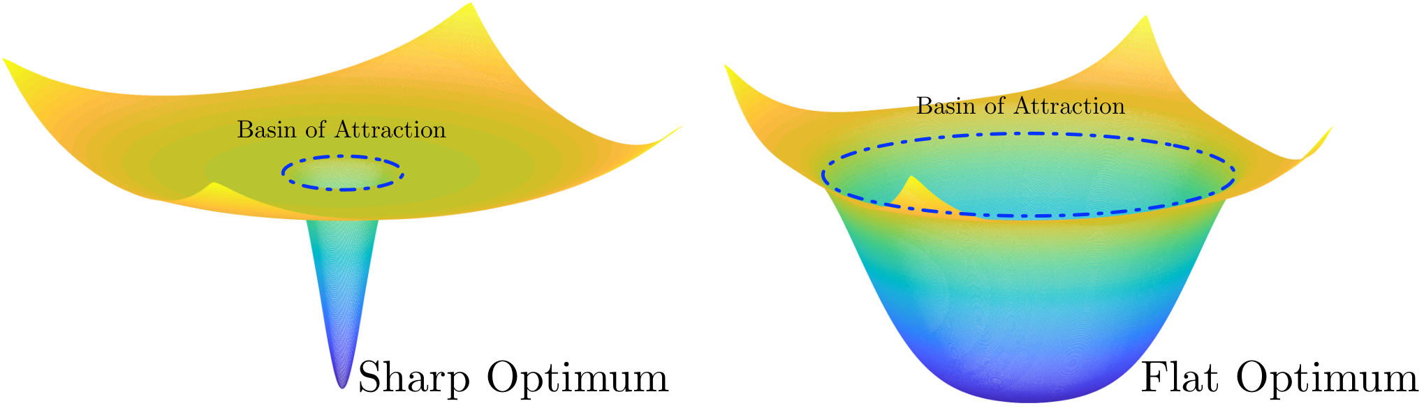
Refer to caption
Figure 5: Two Illustrative Examples of the Flat and Sharp Local Optima. MSGD Tends to Avoid the Sharp Local Optimum, since Its High Variance Encourages Exploration.

∙\bullet Connection to DNNs: The results on training DNNs are expectable or partially expectable, given our theoretical analysis for streaming PCA. Our results show that with a good network architecture, the momentum indeed improves the training.

Our analysis implies that when η\eta is sufficiently small, MSGD with step size η\eta and momentum μ\mu performs similarly to VSGD with step size η1−μ.\frac{\eta}{1-\mu}. In practice, however, people actually use a relative large step size during training and we can still observe the advantage of MSGD over VSGD with the same equivalent step size. As we can observe in Table 2, MSGD always performs better than VSGD. Moreover, MSGD achieves the optimal generalization using ηM1−μ=5.6\frac{\eta_{\rm M}}{1-\mu}=5.6, but VSGD performs the best using a smaller equivalent step size ηV=2.4<5.6\eta_{\rm V}=2.4<5.6 under the ResNet over CIFAR-100. This implies MSGD can afford larger equivalent step size than VSGD. These phenomena cannot be fully explained by our theory.

∙\bullet Flat/Sharp Local Optima: Keskar et al. (2016); Zhang et al. (2017); Neyshabur et al. (2017) suggest that the landscape of these spurious/bad local optima is usually sharp, i.e., their basin of attractions are small and wiggle. From this aspect, using a larger equivalent step size can help MSGD escape from spurious/bad local optima and stay in “flat/good local optima”, since the higher variance of the noise introduced by the momentum encourages more exploration outside the small basin of attraction of sharp local optima.

∙\bullet Extension: Our theoretical analysis can be applied to study other problems related to momentum. For example, Liu et al. (2018) use the main technique of this paper to study an asynchronous MSGD with the focus on the trade off between momentum and asynchrony. For another example, by analyzing the SDE around different local optima, we can theoretically characterize how momentum helps select flat optima.

References

  • Abadi et al. (2016) Abadi, M., Agarwal, A., Barham, P., Brevdo, E., Chen, Z., Citro, C., Corrado, G. S., Davis, A., Dean, J., Devin, M. et al. (2016). Tensorflow: Large-scale machine learning on heterogeneous distributed systems. arXiv preprint arXiv:1603.04467 .
  • Borkar (1997) Borkar, V. S. (1997). Stochastic approximation with two time scales. Systems & Control Letters 29 291–294.
  • Borkar (2009) Borkar, V. S. (2009). Stochastic Approximation: A Dynamical Systems Viewpoint, vol. 48. Springer.
  • Borkar and Meyn (2000) Borkar, V. S. and Meyn, S. P. (2000). The ODE method for convergence of stochastic approximation and reinforcement learning. SIAM Journal on Control and Optimization 38 447–469.
  • Chen et al. (2018) Chen, M., Yang, L., Wang, M. and Zhao, T. (2018). Dimensionality reduction for stationary time series via stochastic nonconvex optimization. In Advances in Neural Information Processing Systems.
  • Chen et al. (2017) Chen, Z., Yang, F. L., Li, C. J. and Zhao, T. (2017). Online multiview representation learning: Dropping convexity for better efficiency. arXiv preprint arXiv:1702.08134 .
  • Choromanska et al. (2015) Choromanska, A., Henaff, M., Mathieu, M., Arous, G. B. and LeCun, Y. (2015). The loss surfaces of multilayer networks. In Artificial Intelligence and Statistics.
  • Fu et al. (2015) Fu, M. C. et al. (2015). Handbook of Simulation Optimization: An Overview of Stochastic Approximation, vol. 216, chap. 6. Springer.
  • Ge et al. (2016) Ge, R., Lee, J. D. and Ma, T. (2016). Matrix completion has no spurious local minimum. In Advances in Neural Information Processing Systems.
  • Ghadimi and Lan (2013) Ghadimi, S. and Lan, G. (2013). Stochastic first-and zeroth-order methods for nonconvex stochastic programming. SIAM Journal on Optimization 23 2341–2368.
  • Ghadimi and Lan (2016) Ghadimi, S. and Lan, G. (2016). Accelerated gradient methods for nonconvex nonlinear and stochastic programming. Mathematical Programming 156 59–99.
  • Goodfellow et al. (2016) Goodfellow, I., Bengio, Y., Courville, A. and Bengio, Y. (2016). Deep learning, vol. 1. MIT press Cambridge.
  • He et al. (2016) He, K., Zhang, X., Ren, S. and Sun, J. (2016). Deep residual learning for image recognition. In Proceedings of the IEEE conference on computer vision and pattern recognition.
  • Hu and Li (2004) Hu, J. and Li, W.-P. (2004). Theory of ordinary differential equations: Existence, uniqueness and stability.
  • Jin et al. (2017) Jin, C., Netrapalli, P. and Jordan, M. I. (2017). Accelerated gradient descent escapes saddle points faster than gradient descent. arXiv preprint arXiv:1711.10456 .
  • Karatzas and Shreve (1998) Karatzas, I. and Shreve, S. E. (1998). Brownian motion. In Brownian Motion and Stochastic Calculus. Springer, 47–127.
  • Keskar et al. (2016) Keskar, N. S., Mudigere, D., Nocedal, J., Smelyanskiy, M. and Tang, P. T. P. (2016). On large-batch training for deep learning: Generalization gap and sharp minima. arXiv preprint arXiv:1609.04836 .
  • Kingma and Ba (2014) Kingma, D. P. and Ba, J. (2014). Adam: A method for stochastic optimization. arXiv preprint arXiv:1412.6980 .
  • Krichene and Bartlett (2017) Krichene, W. and Bartlett, P. L. (2017). Acceleration and averaging in stochastic mirror descent dynamics. arXiv preprint arXiv:1707.06219 .
  • Kushner and Vazquez-Abad (1996) Kushner, H. J. and Vazquez-Abad, F. J. (1996). Stochastic approximation methods for systems over an infinite horizon. SIAM Journal on Control and Optimization 34 712–756.
  • Kushner and Yin (2003) Kushner, H. J. and Yin, G. G. (2003). Stochastic Approximation and Recursive Algorithms and Applications, vol. 35. Springer-Verlag, New York, NY.
  • Li et al. (2017) Li, Q., Tai, C. and Weinan, E. (2017). Stochastic modified equations and adaptive stochastic gradient algorithms. In International Conference on Machine Learning.
  • Li et al. (2016) Li, X., Wang, Z., Lu, J., Arora, R., Haupt, J., Liu, H. and Zhao, T. (2016). Symmetry, saddle points, and global geometry of nonconvex matrix factorization. arXiv preprint arXiv:1612.09296 .
  • Liu et al. (2018) Liu, T., Li, S., Shi, J., Zhou, E. and Zhao, T. (2018). Towards understanding acceleration tradeoff between momentum and asynchrony in distributed nonconvex stochastic optimization. arXiv preprint arXiv:1806.01660 .
  • Matthews et al. (2018) Matthews, A. G. d. G., Rowland, M., Hron, J., Turner, R. E. and Ghahramani, Z. (2018). Gaussian process behaviour in wide deep neural networks. arXiv preprint arXiv:1804.11271 .
  • Mei et al. (2019) Mei, S., Misiakiewicz, T. and Montanari, A. (2019). Mean-field theory of two-layers neural networks: dimension-free bounds and kernel limit. arXiv preprint arXiv:1902.06015 .
  • Mei et al. (2018) Mei, S., Montanari, A. and Nguyen, P.-M. (2018). A mean field view of the landscape of two-layer neural networks. Proceedings of the National Academy of Sciences 115 E7665–E7671.
  • Nesterov (1983) Nesterov, Y. (1983). A method of solving a convex programming problem with convergence rate O⁡(1/k2){O}(1/k^{2}). In Dokl. Akad. Nauk SSSR.
  • Newton et al. (2018) Newton, D., Pasupathy, R. and Yousefian, F. (2018). Recent trends in stochastic gradient descent for machine learning and big data. In Proceedings of the 2018 Winter Simulation Conference. IEEE Press.
  • Neyshabur et al. (2017) Neyshabur, B., Bhojanapalli, S., McAllester, D. and Srebro, N. (2017). Exploring generalization in deep learning. In Advances in Neural Information Processing Systems.
  • Nowakowski (2013) Nowakowski, B. D. (2013). On Multi-parameter Semimartingales, Their Integrals and Weak Convergence.
  • Øksendal (2003) Øksendal, B. (2003). Stochastic differential equations. Springer.
  • Page (2018) Page, D. (2018). How to train your ResNet. https://myrtle.ai/how-to-train-your-resnet/. Accessed: 2018-09-24.
  • Paszke et al. (2019) Paszke, A., Gross, S., Massa, F., Lerer, A., Bradbury, J., Chanan, G., Killeen, T., Lin, Z., Gimelshein, N., Antiga, L. et al. (2019). Pytorch: An imperative style, high-performance deep learning library. In Advances in neural information processing systems.
  • Polyak (1964) Polyak, B. T. (1964). Some methods of speeding up the convergence of iteration methods. USSR Computational Mathematics and Mathematical Physics 4 1–17.
  • Robbins and Monro (1951) Robbins, H. and Monro, S. (1951). A stochastic approximation method. The Annals of Mathematical Statistics 400–407.
  • Rotskoff and Vanden-Eijnden (2018) Rotskoff, G. M. and Vanden-Eijnden, E. (2018). Neural networks as interacting particle systems: Asymptotic convexity of the loss landscape and universal scaling of the approximation error. stat 1050 22.
  • Sagitov (2013) Sagitov, S. (2013). Weak convergence of probability measures. Chalmers University of Technology and Gothenburg University .
  • Simmons (2016) Simmons, G. F. (2016). Differential equations with applications and historical notes. CRC Press.
  • Sirignano and Spiliopoulos (2018) Sirignano, J. and Spiliopoulos, K. (2018). Mean field analysis of neural networks. arXiv preprint arXiv:1805.01053 4.
  • Sirignano and Spiliopoulos (2019) Sirignano, J. and Spiliopoulos, K. (2019). Mean field analysis of deep neural networks. arXiv preprint arXiv:1903.04440 .
  • Sun et al. (2016) Sun, J., Qu, Q. and Wright, J. (2016). A geometric analysis of phase retrieval. In Information Theory (ISIT), 2016 IEEE International Symposium on. IEEE.
  • Sutskever et al. (2013) Sutskever, I., Martens, J., Dahl, G. and Hinton, G. (2013). On the importance of initialization and momentum in deep learning. In International conference on machine learning.
  • Szegedy et al. (2016) Szegedy, C., Vanhoucke, V., Ioffe, S., Shlens, J. and Wojna, Z. (2016). Rethinking the inception architecture for computer vision. In Proceedings of the IEEE Conference on Computer Vision and Pattern Recognition.
  • Wang (2017) Wang, Y. (2017). Asymptotic analysis via stochastic differential equations of gradient descent algorithms in statistical and computational paradigms. arXiv preprint arXiv:1711.09514 .
  • Zhang et al. (2017) Zhang, C., Liao, Q., Rakhlin, A., Sridharan, K., Miranda, B., Golowich, N. and Poggio, T. (2017). Theory of deep learning iii: Generalization properties of SGD. Tech. rep., Center for Brains, Minds and Machines (CBMM).
  • Zhou et al. (2019) Zhou, M., Liu, T., Li, Y., Lin, D., Zhou, E. and Zhao, T. (2019). Toward understanding the importance of noise in training neural networks. In International Conference on Machine Learning. PMLR.

Appendix A Summary on Weak Convergence and Main Theorems

Here, we summarize the theory of weak convergence and theorems used in this paper. Recall that the continuous-time interpolation of the solution trajectory Vη​(⋅)V^{\eta}(\cdot) is defined as Vη​(t)=vkηV^{\eta}(t)=v^{\eta}_{k} on the time interval [kη,kη+η).[k\eta,k\eta+\eta). It has sample paths in the space of Càdlàg functions ( right continuous and have left-hand limits) defined on Rd\mathbb{R}^{d}, or Skorokhod Space, denoted by Dd[0,∞)D^{d}[0,\infty). Thus, the weak convergence we consider here is defined in this space Dd[0,∞)D^{d}[0,\infty) instead of Rd\mathbb{R}^{d}. The special metric σ\sigma in Dd[0,∞)D^{d}[0,\infty) is called Skorokhod metric, and the topology generated by this metric is Skorokhod topology. Please refer to Sagitov (2013); Kushner and Yin (2003) for detailed explanations. The weak convergence in DdD^{d} is defined as follows:

Definition A.1 (Weak Convergence in Dd[0,∞)D^{d}[0,\infty)).

Let ℬ\mathcal{B} be the minimal σ\sigma-field induced by Skorokhod topology. Let {Xn,n<∞}\{X_{n},\,n<\infty\} and XX be random variables on Dd[0,∞)D^{d}[0,\infty) defined on a probability space ( ,P,ℱ).(\Omega,P,\mathcal{F}). Suppose that PnP_{n} and PXP_{X} are the probability measures on (Dd,ℬ)(D^{d},\mathcal{B}) generated by XnX_{n} and X. We say PnP_{n} converges weakly to PP (Pn⇒PP_{n}\Rightarrow P), if for all bounded and continuous real-valued functions FF on DdD^{d}, the following condition holds:

E​F​(Xn)=∫F⁡(x)​d​Pn​(x)→E​F​(X)=∫F⁡(x)​𝑑P​(x)\mathbb{E}F(X_{n})=\intop\nolimits F(x)dP_{n}(x)\rightarrow\mathbb{E}F(X)=\intop\nolimits F(x)dP(x) (A.1)

With an abuse of terminology, we say XnX_{n} converges weakly to XX and write Xn⇒X.X_{n}\Rightarrow X.

Another important definition we need is tightness:

Definition A.2.

A set of DdD^{d}-valued random variables {Xn}\{X_{n}\} is said to be tight if for each δ>0\delta>0, there is a compact set Bδ∈DdB_{\delta}\in D^{d} such that:

supnP{Xn<Bδ}≤δ.\sup_{n}P\{X_{n}\notin B_{\delta}\}\leq\delta. (A.2)

We care about tightness because it provides us a powerful way to prove weak convergence based on the following two theorems:

Theorem A.3 (Prokhorov’s Theorem).

Under Skorokhod topology, {Xn​(⋅)}\{X_{n}(\cdot)\} is tight in Dd[0,∞)D^{d}[0,\infty) if and only if it is relative compact which means each subsequence contains a further subsequence that converges weakly.

Theorem A.4 (Sagitov (2013), Theorem 3.8).

A necessary and sufficient condition for Pn⇒PP_{n}\Rightarrow P is each subsequence Pn′P_{n^{\prime}} contains a further subsequence Pn′′P_{n^{\prime\prime}} converging weakly to P.P.

Thus, if we can prove {Xn​(⋅)}\{X_{n}(\cdot)\} is tight and all the further subsequences share the same weak limit XX, then we have XnX_{n} converges weakly to XX. However, (A.2) is hard to verified. We usually check another easier criteria. We first define the càdlàg modulus to characterize the discontinuity of any f∈Dd​[0,∞].f\in D^{d}[0,\infty].

Definition A.5 (Nowakowski (2013), Definition 2.7).

For f∈Dd​[0,∞],f\in D^{d}[0,\infty], T>0T>0 and ϵ>0,\epsilon>0, the modulus of continuity is defined by

ϖT′​(f,ϵ):=inf�T,ϵmax1≤i≤k⁡w⁡(f,[ti−1,ti)),\varpi^{\prime}_{T}(f,\epsilon):=\inf_{\Pi_{T,\epsilon}}\max_{1\leq i\leq k}w(f,[t_{i-1},t_{i})),

where �T,ϵ={0=t0≤t1≤⋯≤tk=T,min1≤i≤kti−ti−1>ϵ}\Pi_{T,\epsilon}=\{0=t_{0}\leq t_{1}\leq\cdots\leq t_{k}=T,\min_{1\leq i\leq k}t_{i}-t_{i-1}>\epsilon\} and

w⁡(f,[ti−1,ti)):=sups,t∈[ti−1,ti)|f⁡(s)−f⁡(t)|.w(f,[t_{i-1},t_{i})):=\sup_{s,t\in[t_{i-1},t_{i})}|f(s)-f(t)|.

Next theorem provides an sufficient and necessary condition for the tightness of sequence XnX_{n} in Dd[0,∞)D^{d}[0,\infty).

Theorem A.6 (Nowakowski (2013), Theorem 2.4).

Let {Xn​(⋅)}\{X_{n}(\cdot)\} be a sequence of processes that have paths in Dd[0,∞)D^{d}[0,\infty). Then {Xn​(⋅)}\{X_{n}(\cdot)\} is tight if and only if

  • (i).

    For every T>0,T>0, δ>0,\delta>0, there exists n0>0n_{0}>0 and C>0C>0 such that

    P⁡(supt∈[0,T]Xn​(t)>C)≤δ,∀n≥n0.\mathbb{P}\left(\sup_{t\in[0,T]}X_{n}(t)>C\right)\leq\delta,\penalty\ \forall n\geq n_{0}.
  • (ii).

    For every T>0,T>0, δ>0,\delta>0, γ>0,\gamma>0, there exists n0>0n_{0}>0 and ϵ\epsilon such that

    P⁡(ϖT′​(Xn,ϵ)≥γ)≤δ,∀n≥n0.\mathbb{P}\left(\varpi^{\prime}_{T}(X_{n},\epsilon)\geq\gamma\right)\leq\delta,\penalty\ \forall n\geq n_{0}.

Theorem A.7 provides one sufficient condition for tightness. Let ℱtn\mathcal{F}_{t}^{n} be the σ\sigma-algebra generated by {Xn​(s),s≤t}\{X_{n}(s),s\leq t\}, and τ\tau denotes a ℱtn\mathcal{F}_{t}^{n}-stopping time.

Theorem A.7 (Kushner and Yin (2003), Theorem 3.3, Chapter 7).

Let {Xn​(⋅)}\{X_{n}(\cdot)\} be a sequence of processes that have paths in Dd[0,∞)D^{d}[0,\infty). Suppose that for each δ>0\delta>0 and each tt in a dense set in [0,∞)[0,\infty), there is a compact set Kδ,tK_{\delta,t} in R\mathbb{R} such that

infnP{Xn(t)∈Kδ,t}≥1−δ,\inf_{n}P\{X_{n}(t)\in K_{\delta,t}\}\geq 1-\delta, (A.3)

and for each positive TT,

limδlim supnsup|τ|≤Tsups≤δE​min⁡[‖Xn​(τ+s)−Xn​(τ)‖2,1]=0.\lim_{\delta}\limsup_{n}\sup_{|\tau|\leq T}\sup_{s\leq\delta}\mathbb{E}\min[\|X_{n}(\tau+s)-X_{n}(\tau)\|_{2},1]=0. (A.4)

Then {Xn​(⋅)}\{X_{n}(\cdot)\} is tight in Dd[0,∞).D^{d}[0,\infty).

This theorem is used in Section 3 to prove tightness of the trajectory of Momentum SGD.

At last, we provide the theorem we use to prove the SDE approximation. Let’s consider the following algorithm:

θn+1η=θnη+η​Ynη,\theta_{n+1}^{\eta}=\theta_{n}^{\eta}+\eta Y_{n}^{\eta}, (A.5)

where Ynη=gnη​(θnη,ξnη)+MnηY_{n}^{\eta}=g_{n}^{\eta}(\theta_{n}^{\eta},\xi_{n}^{\eta})+M_{n}^{\eta}, and MnηM_{n}^{\eta} is a martingale difference sequence. Then the normalized process Unη=(θnη−θ¯)/ηU_{n}^{\eta}=(\theta_{n}^{\eta}-\bar{\theta})/\sqrt{\eta} satisfies:

Un+1η=Unη+η​(gnη​(θnη,ξnη)+Mnη).U_{n+1}^{\eta}=U_{n}^{\eta}+\sqrt{\eta}(g_{n}^{\eta}(\theta_{n}^{\eta},\xi_{n}^{\eta})+M_{n}^{\eta}). (A.6)

We further assume the fixed-state-chain exists and use the same notation ξi​(θ)\xi_{i}(\theta) to denote the fixed-θ\theta-process. Then we have the following theorem:

Theorem A.8 (Kushner and Yin (2003), Theorem 8.1, Chapter 10).

Assume the following conditions hold:

  1. C.1

    For small ρ>0\rho>0, {|Ynη|2​I|θnη−θ¯|≤ρ}\{|Y_{n}^{\eta}|^{2}I_{|\theta_{n}^{\eta}-\bar{\theta}|\leq\rho}\} is uniformly integrable.

  2. C.2

    There is a continuous function g¯​(⋅)\bar{g}(\cdot) such that for any sequence of integers nη→0n_{\eta}\rightarrow 0 satisfying nη​η→0n_{\eta}\eta\rightarrow 0 as η→0\eta\rightarrow 0 and each compact set AA,

    1nη​∑i=j​nηj​nη+nη−1Ej​nηη​[giη​(θ,ξi​(θ))−g¯​(θ)]​I{ξj​nηη}→0\frac{1}{n_{\eta}}\sumop\displaylimits_{i=jn_{\eta}}^{jn_{\eta}+n_{\eta}-1}E_{jn_{\eta}}^{\eta}[g_{i}^{\eta}(\theta,\xi_{i}(\theta))-\bar{g}(\theta)]I_{\{\xi_{jn_{\eta}}^{\eta}\}}\rightarrow 0

    in the mean for each θ\theta, as j→∞j\rightarrow\infty and η→0.\eta\rightarrow 0.

  3. C.3

    Define

    �nη​(θ)=∑i=n∞(1−η)i−n​Enη​[giη​(θ,ξi​(θ))−g¯​(θ)],\Gamma_{n}^{\eta}(\theta)=\sumop\displaylimits_{i=n}^{\infty}(1-\eta)^{i-n}E_{n}^{\eta}[g_{i}^{\eta}(\theta,\xi_{i}(\theta))-\bar{g}(\theta)],

    where when EnηE_{n}^{\eta} is used, the initial condition is ξn​(θ)=ξnη.\xi_{n}(\theta)=\xi_{n}^{\eta}. For the initial conditions ξnη\xi_{n}^{\eta} confined to any compact set,

    {|�nη​(θnη)|2​I|θnη−θ¯|≤ρ,|�nη​(θ¯)|2;n,η}\{|\Gamma_{n}^{\eta}(\theta_{n}^{\eta})|^{2}I_{|\theta_{n}^{\eta}-\bar{\theta}|\leq\rho},|\Gamma_{n}^{\eta}(\bar{\theta})|^{2};n,\eta\}

    is uniformly integrable, and

    E​|Enη​�n+1η​(θn+1η)−�n+1η​(θnη)|2​I|θnη−θ¯|≤ρ=O⁡(η2).E\left|E_{n}^{\eta}\Gamma_{n+1}^{\eta}(\theta_{n+1}^{\eta})-\Gamma_{n+1}^{\eta}(\theta_{n}^{\eta})\right|^{2}I_{|\theta_{n}^{\eta}-\bar{\theta}|\leq\rho}=O(\eta^{2}).
  4. C.4

    There is a Hurwitz matrix AA such that

    g¯​(θ)=A⁡(θ−θ¯)+o⁡(θ−θ¯).\bar{g}(\theta)=A(\theta-\bar{\theta})+o(\theta-\bar{\theta}).
  5. C.5

    There is a matrix �0={σ0,i​j;i,j=i,…,r}\Sigma_{0}=\{\sigma_{0,ij};\,i,j=i,...,r\} such that as n,m→∞,n,m\rightarrow\infty,

    1m​∑i=nn+m−1Enη​[Miη​(Miη)′−�0]​I|θnη−θ¯|≤ρ→0\frac{1}{m}\sumop\displaylimits_{i=n}^{n+m-1}E_{n}^{\eta}[M_{i}^{\eta}(M_{i}^{\eta})^{\prime}-\Sigma_{0}]I_{|\theta_{n}^{\eta}-\bar{\theta}|\leq\rho}\rightarrow 0

    in probability.

Then {Uη​(⋅)}\{U^{\eta}(\cdot)\} is tight. Given tightness, we further assumes the following assumptions hold.

  1. C.6

    There is a matrix �¯0={σ¯0,i​j;i,j=i,…,r}\bar{\Sigma}_{0}=\{\bar{\sigma}_{0,ij};\,i,j=i,...,r\} such that as n,m→∞,n,m\rightarrow\infty,

    1m​∑i=nn+m−1Enη​[giη​(θ¯,ξi​(θ¯))​(giη​(θ¯,ξi​(θ¯)))′−�¯0]→0\frac{1}{m}\sumop\displaylimits_{i=n}^{n+m-1}E_{n}^{\eta}[g_{i}^{\eta}(\bar{\theta},\xi_{i}(\bar{\theta}))(g_{i}^{\eta}(\bar{\theta},\xi_{i}(\bar{\theta})))^{\prime}-\bar{\Sigma}_{0}]\rightarrow 0

    in probability.

  2. C.7

    Define another function

    Gnη,i​(θ,ξnη)=Enη​[�n+1η​(θnη)​[Ynη]′​I|θnη−θ¯|≤ρ|θnη=θ].G_{n}^{\eta,i}(\theta,\xi_{n}^{\eta})=E_{n}^{\eta}\left[\Gamma_{n+1}^{\eta}(\theta_{n}^{\eta})[Y_{n}^{\eta}]^{\prime}I_{|\theta_{n}^{\eta}-\bar{\theta}|\leq\rho}\big|\theta_{n}^{\eta}=\theta\right].

    It needs to be a continuous function in (θ,ξnη)(\theta,\xi_{n}^{\eta}), uniformly in nn and η\eta.

  3. C.8

    There is a matrix �1={σ1,i​j;i,j=i,…,r}\Sigma_{1}=\{\sigma_{1,ij};\,i,j=i,...,r\} such that as n,m→∞,n,m\rightarrow\infty,

    1m​∑i=nn+m−1Enη​[Gnη,i​(θ¯,ξi​(θ¯))−�1]→0\frac{1}{m}\sumop\displaylimits_{i=n}^{n+m-1}E_{n}^{\eta}[G_{n}^{\eta,i}(\bar{\theta},\xi_{i}(\bar{\theta}))-\Sigma_{1}]\rightarrow 0

    in probability.

Then there exists a Wiener process W⁡(⋅)W(\cdot) with covariance matrix �=�0+�¯0+�1+�1′\Sigma=\Sigma_{0}+\bar{\Sigma}_{0}+\Sigma_{1}+\Sigma_{1}^{\prime} such that {Uη​(⋅)}\{U^{\eta}(\cdot)\} converges weakly to a stationary solution of

d​U=A​U​d​t+d​W.dU=AUdt+dW.

Appendix B Proof of Theorem 3.1

The proof consists of two parts. In the first part, we show that {Xη​(⋅)}\{X^{\eta}(\cdot)\} is tight. Therefore, every sub-sequence has further one sub-sequence that weakly converges to some limit process. In the second part, we find the limit ODE and show that the solution to this ODE exists and is unique. Combining these two parts, we prove the result.

∙\bullet Tightness. We first rewrite MSGD as follows:

xk+1η=x1η−η​∑j=1k∑i=1jμj−i​f​(xiη,ξiη).x_{k+1}^{\eta}=x_{1}^{\eta}-\eta\sumop\displaylimits_{j=1}^{k}\sumop\displaylimits_{i=1}^{j}\mu^{j-i}f(x_{i}^{\eta},\xi_{i}^{\eta}).

Under Assumption 1, we have

‖xkη‖2≤||x1η||2+η​∑j=1k∑i=1jμj−i​C≤‖x1η‖2+C​k​η1−μ.||x_{k}^{\eta}||_{2}\leq||x_{1}^{\eta}||_{2}+\eta\sumop\displaylimits_{j=1}^{k}\sumop\displaylimits_{i=1}^{j}\mu^{j-i}C\leq||x_{1}^{\eta}||_{2}+\frac{Ck\eta}{1-\mu}.

Then the continuous interpolation Xη​(t)X^{\eta}(t) satisfies:

‖Xη​(t)‖2≤||x1η||2+tη​C​η1−μ=‖x1η‖2+C​t1−μ.||X^{\eta}(t)||_{2}\leq||x_{1}^{\eta}||_{2}+\frac{t}{\eta}\frac{C\eta}{1-\mu}=||x_{1}^{\eta}||_{2}+\frac{Ct}{1-\mu}.

We define Kδ,t={x|‖x‖2≤‖x1η‖2+C​t1−μ}K_{\delta,t}=\left\{x\Big|||x||_{2}\leq||x_{1}^{\eta}||_{2}+\frac{Ct}{1-\mu}\right\}. Then for any δ>0,t>0\delta>0,t>0 we have

infηP{Xη(t)∈Kδ,t}=1≥1−δ.\inf_{\eta}\mathbb{P}\{X^{\eta}(t)\in K_{\delta,t}\}=1\geq 1-\delta.

Moreover, ∀τ,s>0,\forall\tau,s>0, we have

‖Xη​(τ+s)−Xη​(τ)‖2≤C​s1−μ.||X^{\eta}(\tau+s)-X^{\eta}(\tau)||_{2}\leq\frac{Cs}{1-\mu}.

Therefore, for each positive TT,

limδlim supηsup|τ|≤Tsups≤δE​min⁡[‖Xη​(τ+s)−Xη​(τ)‖2,1]=0.\lim_{\delta}\limsup_{\eta}\sup_{|\tau|\leq T}\sup_{s\leq\delta}\mathbb{E}\min[\|X^{\eta}(\tau+s)-X^{\eta}(\tau)\|_{2},1]=0.

Then by Theorem A.7, {Xη​(⋅)}\{X^{\eta}(\cdot)\} is tight.

∙\bullet Limit Process. For simplicity, we define

βkη=∑i=0k−1μk−i​(∇f​(xiη,ξi)−∇ℱ​(xiη))andϵk=∇f​(xkη,ξk)−∇ℱ​(xkη).\displaystyle\textstyle\beta_{k}^{\eta}=\sumop\displaylimits_{i=0}^{k-1}\mu^{k-i}(\nabla f(x_{i}^{\eta},\xi_{i})-\nabla\mathcal{F}(x_{i}^{\eta}))\penalty\ \penalty\ \text{and}\penalty\ \penalty\ \epsilon_{k}=\nabla f(x_{k}^{\eta},\xi_{k})-\nabla\mathcal{F}(x_{k}^{\eta}).

We then rewrite the algorithm as follows:

mk+1η=mkη+(1−μ)​[−mkη+M~​(xkη)],xk+1η=xkη+η​(mk+1η+βkη+ϵkη),\displaystyle m_{k+1}^{\eta}=m_{k}^{\eta}+(1-\mu)\left[-m_{k}^{\eta}+\widetilde{M}(x_{k}^{\eta})\right],\penalty\ \penalty\ x_{k+1}^{\eta}=x_{k}^{\eta}+\eta(m_{k+1}^{\eta}+\beta_{k}^{\eta}+\epsilon_{k}^{\eta}),

where M~(xkη)=−11−μ∇ℱ(xkη)\widetilde{M}(x_{k}^{\eta})=-\frac{1}{1-\mu}\nabla\mathcal{F}(x_{k}^{\eta}) is the rescaled negative gradient and

mk+1\displaystyle m_{k+1} =−∑i=0kμi∇ℱ(xiη).\displaystyle=-\sumop\displaylimits_{i=0}^{k}\mu^{i}\nabla\mathcal{F}(x_{i}^{\eta}).

Define the sums

ℰη​(t)=η​∑i=0t/η−1ϵiη,Bη​(t)=η​∑i=0t/η−1βiη,\displaystyle\mathcal{E}^{\eta}(t)=\eta\sumop\displaylimits_{i=0}^{t/\eta-1}\epsilon_{i}^{\eta},\quad B^{\eta}(t)=\eta\sumop\displaylimits_{i=0}^{t/\eta-1}\beta_{i}^{\eta},
G¯η​(t)=η​∑i=0t/η−1M~​(xiη),G~η​(t)=η​∑i=0t/η−1[mi+1η−M~​(xiη)].\displaystyle\bar{G}^{\eta}(t)=\eta\sumop\displaylimits_{i=0}^{t/\eta-1}\widetilde{M}(x_{i}^{\eta}),\quad\widetilde{G}^{\eta}(t)=\eta\sumop\displaylimits_{i=0}^{t/\eta-1}[m_{i+1}^{\eta}-\widetilde{M}(x_{i}^{\eta})].

Then the continuous-time interpolation of Xη​(t)X^{\eta}(t) can be decomposed as follows.

Xη​(t)=x0η+G¯η​(t)+G~η​(t)+Bη​(t)+ℰη​(t).X^{\eta}(t)=x^{\eta}_{0}+\bar{G}^{\eta}(t)+\widetilde{G}^{\eta}(t)+B^{\eta}(t)+\mathcal{E}^{\eta}(t).

Define the process Wη​(t)W^{\eta}(t) by

Wη​(t)=Xη​(t)−x0η−G¯η​(t)=G~η​(t)+Bη​(t)+ℰη​(t).W^{\eta}(t)=X^{\eta}(t)-x^{\eta}_{0}-\bar{G}^{\eta}(t)=\widetilde{G}^{\eta}(t)+B^{\eta}(t)+\mathcal{E}^{\eta}(t).

We have already shown that {Xη(⋅))}\{X^{\eta}(\cdot))\} is tight in the first part of the proof. Specifically, there is a subsequence η​(k)→0\eta(k)\rightarrow 0 and a process X⁡(⋅)X(\cdot) such that

Xη​(k)​(t)⇒X​(t),X^{\eta(k)}(t)\Rightarrow X(t),

as k→∞.k\rightarrow\infty. Under the bounded assumption of ∇f​(x,ξ),\nabla f(x,\xi), one can show that

‖xk+1η−xkη‖2=η​‖∑i=1kμj−i​f​(xiη,ξiη)‖2≤η1−μ​C,||x_{k+1}^{\eta}-x^{\eta}_{k}||_{2}=\eta||\sumop\displaylimits_{i=1}^{k}\mu^{j-i}f(x^{\eta}_{i},\xi_{i}^{\eta})||_{2}\leq\frac{\eta}{1-\mu}C,

which further implies the uniform integrability of {xkη}\{x_{k}^{\eta}\}. By Lemma 2.1 in Kushner and Vazquez-Abad (1996), we know that any weak sense limit X⁡(t)X(t) must have Lipschitz continuous path. For notational simplicity, we write η​(k)\eta(k) as η\eta in the following proof.

For t>0t>0 and integer pp, we take si≤t,s_{i}\leq t, i≤p,i\leq p, and τ>0\tau>0. Let g⁡(⋅)g(\cdot) be a continuous, bounded and real-valued function. Then by definition of Wη​(t)W^{\eta}(t), we have

0=E\displaystyle 0=E g⁡(Xη​(si),i≤p)​[Wη​(t+τ)−Wη​(t)]\displaystyle g(X^{\eta}(s_{i}),i\leq p)[W^{\eta}(t+\tau)-W^{\eta}(t)] (B.1)
−E​g​(Xη​(si),i≤p)​[G~η​(t+τ)−G~η​(t)]\displaystyle-Eg(X^{\eta}(s_{i}),i\leq p)[\widetilde{G}^{\eta}(t+\tau)-\widetilde{G}^{\eta}(t)] (B.2)
−E​g​(Xη​(si),i≤p)​[ℰη​(t+τ)−ℰη​(t)]\displaystyle-Eg(X^{\eta}(s_{i}),i\leq p)[\mathcal{E}^{\eta}(t+\tau)-\mathcal{E}^{\eta}(t)] (B.3)
−E​g​(Xη​(si),i≤p)​[Bη​(t+τ)−Bη​(t)].\displaystyle-Eg(X^{\eta}(s_{i}),i\leq p)[B^{\eta}(t+\tau)-B^{\eta}(t)]. (B.4)

Let ℱnη=σ​{xiη,ξi−1η,i≤n},\mathcal{F}^{\eta}_{n}=\sigma\{x^{\eta}_{i},\xi_{i-1}^{\eta},i\leq n\}, then ℱt/ηη\mathcal{F}^{\eta}_{t/\eta} measures {ℰη​(s),s≤t}\{\mathcal{E}^{\eta}(s),s\leq t\} by definition and the process ℰη​(⋅)\mathcal{E}^{\eta}(\cdot) is actually an ℱt/ηη\mathcal{F}^{\eta}_{t/\eta}-martingale. By the tower property of the conditional expectation, we know term (B.3) equals to 0.
Next, we eliminate term (B.4). Note that for any m,n>0m,n>0, we have

‖1m​∑i=nn+m−1E⁡[βiη|ℱn]‖2=‖1m​∑i=nn+m−1μi−n​βnη‖2≤1(1−μ)​m​‖βnη‖2.\left\|\frac{1}{m}\sumop\displaylimits_{i=n}^{n+m-1}\mathbb{E}[\beta^{\eta}_{i}|\mathcal{F}_{n}]\right\|_{2}=\left\|\frac{1}{m}\sumop\displaylimits_{i=n}^{n+m-1}\mu^{i-n}\beta^{\eta}_{n}\right\|_{2}\leq\frac{1}{(1-\mu)m}\|\beta^{\eta}_{n}\|_{2}.

Since βnη\beta^{\eta}_{n} is uniformly bounded in η,m\eta,m and nn, we have

limm,n,η1m​∑i=nn+m−1E⁡[βiη|ℱn]=0\lim_{m,n,\eta}\frac{1}{m}\sumop\displaylimits_{i=n}^{n+m-1}\mathbb{E}[\beta^{\eta}_{i}|\mathcal{F}_{n}]=0

in ℒ2\mathcal{L}_{2}, which also means

limη→0E⁡[Bη​(t+τ)−Bη​(t)|ℱt/ηη]=0.\lim_{\eta\rightarrow 0}\mathbb{E}[B^{\eta}(t+\tau)-B^{\eta}(t)|\mathcal{F}^{\eta}_{t/\eta}]=0.

Together with the boundedness of ff, by Dominated Convergence Theorem, we know that term (B.4) goes to 0, as η→0\eta\rightarrow 0.

For term (B.2), we first bound ‖G~η​(t+τ)−G~η​(t)‖2.\|\widetilde{G}^{\eta}(t+\tau)-\widetilde{G}^{\eta}(t)\|_{2}. Since 11−μ=∑i=0∞μi\frac{1}{1-\mu}=\sumop\displaylimits_{i=0}^{\infty}\mu^{i}, there exists N⁡(η)=logμ⁡(1−μ)​ηN(\eta)=\log_{\mu}(1-\mu)\eta such that ∑i=N⁡(η)∞μi<η.\sumop\displaylimits_{i=N(\eta)}^{\infty}\mu^{i}<\eta. When k>N⁡(η)k>N(\eta), write mkηm_{k}^{\eta} and M~​(xkη)\widetilde{M}(x_{k}^{\eta}) into summations:

mk+1η=−∑i=0kμi∇ℱ(xiη)=−∑i=0N⁡(η)μi∇ℱ(xiη)−∑i=N⁡(η)+1kμi∇ℱ(xiη),\displaystyle m^{\eta}_{k+1}=-\sumop\displaylimits_{i=0}^{k}\mu^{i}\nabla\mathcal{F}(x_{i}^{\eta})=-\sumop\displaylimits_{i=0}^{N(\eta)}\mu^{i}\nabla\mathcal{F}(x_{i}^{\eta})-\sumop\displaylimits_{i=N(\eta)+1}^{k}\mu^{i}\nabla\mathcal{F}(x_{i}^{\eta}),

and

M~(xkη)=−11−μ∇ℱ(xkη)=−∑i=0N⁡(η)μi∇ℱ(xkη)−∑i=N⁡(η)+1∞μi∇ℱ(xkη).\displaystyle\widetilde{M}(x_{k}^{\eta})=-\frac{1}{1-\mu}\nabla\mathcal{F}(x_{k}^{\eta})=-\sumop\displaylimits_{i=0}^{N(\eta)}\mu^{i}\nabla\mathcal{F}(x_{k}^{\eta})-\sumop\displaylimits_{i=N(\eta)+1}^{\infty}\mu^{i}\nabla\mathcal{F}(x_{k}^{\eta}).

Note that ‖xk+1η−xkη‖2≤C1−μ​η\|x_{k+1}^{\eta}-x_{k}^{\eta}\|_{2}\leq\frac{C}{1-\mu}\eta. Then we have

maxi=0,1,…,N⁡(η)⁡‖xk−iη−xkη‖2≤C1−μ​N​(η)​η→0,\max_{i=0,1,...,N(\eta)}\|x_{k-i}^{\eta}-x_{k}^{\eta}\|_{2}\leq\frac{C}{1-\mu}N(\eta)\eta\rightarrow 0,

as η→0\eta\rightarrow 0. By the Lipschitz assumption, for i=0,1,…,N⁡(δ),i=0,1,...,N(\delta), we have

‖∇ℱ​(xkη)−∇ℱ​(xk−iη)‖2≤L​C1−μ​N​(η)​η.\|\nabla\mathcal{F}(x_{k}^{\eta})-\nabla\mathcal{F}(x_{k-i}^{\eta})\|_{2}\leq L\frac{C}{1-\mu}N(\eta)\eta.

Then

‖∑i=0N⁡(η)μi​{∇ℱ​(xk−iη)−∇ℱ​(xkη)}‖2≤L​C​N​(η)​η(1−μ)2.\left\|\sumop\displaylimits_{i=0}^{N(\eta)}\mu^{i}\{\nabla\mathcal{F}(x_{k-i}^{\eta})-\nabla\mathcal{F}(x_{k}^{\eta})\}\right\|_{2}\leq\frac{LCN(\eta)\eta}{(1-\mu)^{2}}.

Since ∇ℱ​(xkη)\nabla\mathcal{F}(x_{k}^{\eta}) is bounded by CC, both ∑i=N⁡(η)+1kμi∇ℱ(xk−iη)\sumop\displaylimits_{i=N(\eta)+1}^{k}\mu^{i}\nabla\mathcal{F}(x_{k-i}^{\eta}) and ∑i=N⁡(η)+1∞μi∇ℱ(xkη)\sumop\displaylimits_{i=N(\eta)+1}^{\infty}\mu^{i}\nabla\mathcal{F}(x_{k}^{\eta}) are bounded by C​η.C\eta. Thus,

‖mk+1η−M~​(xkη)‖2≤K​C​N​(η)​η1−μ+2​C​η=O⁡(η​log⁡1η).\|m^{\eta}_{k+1}-\widetilde{M}(x^{\eta}_{k})\|_{2}\leq\frac{KCN(\eta)\eta}{1-\mu}+2C\eta=O\left(\eta\log\frac{1}{\eta}\right).

For k<N⁡(η)k<N(\eta), following the same approach, we can bound ‖mk+1η−M~​(mkη)‖2\|m^{\eta}_{k+1}-\widetilde{M}(m^{\eta}_{k})\|_{2} by the same bound O⁡(η​log⁡1η)O\left(\eta\log\frac{1}{\eta}\right). Therefore, we have the following bound for ‖G~η​(t+τ)−G~η​(t)‖2.\|\widetilde{G}^{\eta}(t+\tau)-\widetilde{G}^{\eta}(t)\|_{2}.

‖G~η​(t+τ)−G~η​(t)‖2≤τ​O​(η​log⁡1η).\|\widetilde{G}^{\eta}(t+\tau)-\widetilde{G}^{\eta}(t)\|_{2}\leq\tau O\left(\eta\log\frac{1}{\eta}\right).

Thus, term (B.2) goes to 0 as η→0\eta\rightarrow 0. Then we have

limηE​g​(Xη​(si),i≤p)​[Wη​(t+τ)−Wη​(t)]=0.\lim_{\eta}Eg(X^{\eta}(s_{i}),i\leq p)[W^{\eta}(t+\tau)-W^{\eta}(t)]=0.

Define

W⁡(t)=X⁡(t)−X⁡(0)−∫0TM~​(X⁡(s))​𝑑s.W(t)=X(t)-X(0)-\intop\nolimits_{0}^{T}\widetilde{M}(X(s))ds.

Then the weak convergence and the previous analysis together imply that

E​g​(Xη​(si),i≤p)​[W⁡(t+τ)−W⁡(t)]=0.Eg(X^{\eta}(s_{i}),i\leq p)[W(t+\tau)-W(t)]=0.

Here, we need an important result in the martingale theory:

Theorem B.1 (Kushner and Yin (2003), Theorem 4.1, Chapter 7).

Let U⁡(⋅)U(\cdot) be a random process with paths in Dd[0,∞)D^{d}[0,\infty), where U⁡(t)U(t) is measurable on the σ\sigma-algebra ℱtX\mathcal{F}_{t}^{X} determined by {X⁡(s),s≤t}\{X(s),s\leq t\} for some given process X⁡(⋅)X(\cdot) and let E⁡[U⁡(t)]<∞\mathbb{E}[U(t)]<\infty for each tt. Suppose that for each real t≥0t\geq 0 and τ≥0\tau\geq 0, each integer pp and each set of real numbers si≤t,i=1,…,p,s_{i}\leq t,\,i=1,...,p, and each bounded and continuous real-valued function h⁡(⋅)h(\cdot),

E​h​(Xη​(si),i≤p)​[U⁡(t+τ)−U⁡(t)]=0,Eh(X^{\eta}(s_{i}),i\leq p)[U(t+\tau)-U(t)]=0,

then U⁡(t)U(t) is a ℱtX\mathcal{F}_{t}^{X}-martingale.

By Theorem B.1 , we know that W⁡(⋅)W(\cdot) is a martingale. It has locally Lipschitz continuous sample paths by the fact X⁡(⋅)X(\cdot) is Lipschitz. Since a Lipschitz continuous martingale must almost surely be a constant, we know W⁡(t)=W⁡(0)=0W(t)=W(0)=0 with probability 1. In other words, X⁡(t)X(t) is a solution to the following ODE

X˙=−11−μ∇ℱ(x),x(0)=x0.\displaystyle\dot{X}=-\frac{1}{1-\mu}\nabla\mathcal{F}(x),\quad x(0)=x_{0}. (B.5)

Moreover, under Assumption 1 and by Theorem 12.70.B in Simmons (2016), we know that the above initial value problem has only one solution. Therefore, all sub-sequences of {Xη​(⋅)}\{X^{\eta}(\cdot)\} weakly converge to the same limit, which implies the weak convergence of the entire sequence. We prove the theorem.

Appendix C Detailed Proof in Section 4

C.1 Proof of Theorem 4.2

Proof.

The proof follows from Theorem 10.8.1 in Kushner and Yin (2003) (Theorem A.8). We need to check the Assumption C.1 to C.8 (in Appendix A)

  • 1.

    The uniform integrability in C.1 directly follows from the uniform boundedness assumption of ∇f​(x,ξ)\nabla f(x,\xi).

  • 2.

    C.2 can be easily got from the proof of ODE approximation.

  • 3.

    To check condition C.4, we need use our isolated stationary point assumption, i.e, Assumption 2. At the local optimum x∗,x^{*}, the Hessian matrix must be positive definite. Then C.4 is obviously satisfied with the Hurwitz matrix −∇2ℱ​(x∗).-\nabla^{2}\mathcal{F}(x^{*}).

The main challenge left is to calculate the variance of the Wiener process and check the other five assumptions.

For simplicity, Ekη​[⋅]E_{k}^{\eta}[\cdot] means the conditional expectation for

{ζk+j,j≥0;ζk​(X)=ζkη}.\{\zeta_{k+j},j\geq 0;\zeta_{k}(X)=\zeta_{k}^{\eta}\}.

From Equation (4.2), the variance can be decomposed into three parts. The first part is from the noise γkη,i\gamma_{k}^{\eta,i}. Since we have assumed the weak convergence xkη⇒x∗x_{k}^{\eta}\Rightarrow x^{*}, we have in distribution,

limη,kEkη​(γk+jη​(γk+jη)⊤)=�.\displaystyle\lim_{\eta,k}E_{k}^{\eta}(\gamma_{k+j}^{\eta}(\gamma_{k+j}^{\eta})^{\top})=\Sigma.

Since the limit is a constant, the convergence also holds in probability. Thus, C.5 is satisfied. The second part comes from the fixed-state-chain:

Ekη​(g⁡(x∗,ζk+jη​(x∗))​g​(x∗,ζk+jη​(x∗))⊤)\displaystyle E_{k}^{\eta}(g(x^{*},\zeta_{k+j}^{\eta}(x^{*}))g(x^{*},\zeta_{k+j}^{\eta}(x^{*}))^{\top}) =Ekη​(ζk+jη​(x∗)−∇F​(x∗))​(ζk+jη​(x∗)−∇F​(x∗))⊤\displaystyle=E_{k}^{\eta}(\zeta_{k+j}^{\eta}(x^{*})-\nabla F(x^{*}))(\zeta_{k+j}^{\eta}(x^{*})-\nabla F(x^{*}))^{\top}
=Ekη​ζk+jη​(x∗)​(ζk+jη​(x∗))⊤\displaystyle=E_{k}^{\eta}\zeta_{k+j}^{\eta}(x^{*})(\zeta_{k+j}^{\eta}(x^{*}))^{\top}
=μ2​j(ζkη)(ζkη)⊤+∑m=0j−1μ2​(j−m)Ekη[∇f(x∗,ξk+m)∇f(x∗,ξk+m)⊤]\displaystyle=\mu^{2j}(\zeta^{\eta}_{k})(\zeta^{\eta}_{k})^{\top}+\sumop\displaylimits_{m=0}^{j-1}\mu^{2(j-m)}E_{k}^{\eta}[\nabla f(x^{*},\xi_{k+m})\nabla f(x^{*},\xi_{k+m})^{\top}]
→μ21−μ2​�,\displaystyle\rightarrow\frac{\mu^{2}}{1-\mu^{2}}\Sigma,

in probability, as k,j→0.k,j\rightarrow 0. Thus, C.6 is satisfied.

The last part is from the term g⁡(ζkη,xkη)−g⁡(ζk​(xkη),xkη)g(\zeta_{k}^{\eta},x_{k}^{\eta})-g(\zeta_{k}(x_{k}^{\eta}),x_{k}^{\eta}). Define the discounted sequence

�kη​(x)=∑j=0∞(1−η)j​Ekη​[g⁡(x,ζk+jη​(x))−M~​(x)].\Gamma_{k}^{\eta}(x)=\sumop\displaylimits_{j=0}^{\infty}(1-\eta)^{j}E_{k}^{\eta}[g(x,\zeta_{k+j}^{\eta}(x))-\widetilde{M}(x)].

Note that

Ekη​[ζk+jη​(x)]\displaystyle E_{k}^{\eta}[\zeta_{k+j}^{\eta}(x)] =Ekη[μjζkη−∑m=0j−1μj−m∇f(x,ξk+m)]\displaystyle=E_{k}^{\eta}[\mu^{j}\zeta_{k}^{\eta}-\sumop\displaylimits_{m=0}^{j-1}\mu^{j-m}\nabla f(x,\xi_{k+m})]
=μjζkη−∑m=0j−1μj−m∇ℱ(x).\displaystyle=\mu^{j}\zeta_{k}^{\eta}-\sumop\displaylimits_{m=0}^{j-1}\mu^{j-m}\nabla\mathcal{F}(x).

Thus, we have

Ekη[g(x,ζk+jη(x))−M~(x)]=μjζkη+μj+11−μ∇ℱ(x).E_{k}^{\eta}[g(x,\zeta_{k+j}^{\eta}(x))-\widetilde{M}(x)]=\mu^{j}\zeta_{k}^{\eta}+\frac{\mu^{j+1}}{1-\mu}\nabla\mathcal{F}(x).

Then

�kη(x)=∑j=0∞(1−η)j{μjζkη+μj+11−μ∇ℱ(x)}=11−(1−η)​μ(ζkη−μ1−μM~(x)).\Gamma_{k}^{\eta}(x)=\sumop\displaylimits_{j=0}^{\infty}(1-\eta)^{j}\left\{\mu^{j}\zeta_{k}^{\eta}+\frac{\mu^{j+1}}{1-\mu}\nabla\mathcal{F}(x)\right\}=\frac{1}{1-(1-\eta)\mu}\left(\zeta_{k}^{\eta}-\frac{\mu}{1-\mu}\widetilde{M}(x)\right).

Since M{M} is locally Lipschitz, and ‖xk+1η−xkη‖2=O⁡(η)\|x_{k+1}^{\eta}-x_{k}^{\eta}\|_{2}=O(\eta), the following result holds:

‖Ekη​[�k+1η​(xk+1η)−�k+1η​(xkη)]‖22\displaystyle\|E_{k}^{\eta}[\Gamma_{k+1}^{\eta}(x_{k+1}^{\eta})-\Gamma_{k+1}^{\eta}(x_{k}^{\eta})]\|_{2}^{2} =‖μ(1−(1−η)​μ)​(1−μ)​{Ekη​[M~​(xk+1η)−M~​(xkη)]}‖22\displaystyle=\left\|\frac{\mu}{(1-(1-\eta)\mu)(1-\mu)}\left\{E_{k}^{\eta}[\widetilde{M}(x_{k+1}^{\eta})-\widetilde{M}(x_{k}^{\eta})]\right\}\right\|_{2}^{2}
=O⁡(η2).\displaystyle=O(\eta^{2}).

Then, Assumption C.3 holds.

Define another function

Gkη​(x,ζkη)=Ekη​[�k+1η,i​(xkη)​(Zkη)⊤|xkη=x].G_{k}^{\eta}(x,\zeta_{k}^{\eta})=E_{k}^{\eta}\left[\Gamma_{k+1}^{\eta,i}(x_{k}^{\eta})(Z_{k}^{\eta})^{\top}|x_{k}^{\eta}=x\right].

It is easy to check this is a continuous function in (x,ζkη)(x,\zeta_{k}^{\eta}), uniformly in kk and η\eta (Assumption C.7). Moreover,

�k+1η​(xkη)​(Zkη)⊤\displaystyle\Gamma_{k+1}^{\eta}(x_{k}^{\eta})(Z_{k}^{\eta})^{\top} =11−(1−η)​μ​(ζk+1η−μ1−μ​M~​(xkη))​1μ​(ζk+1η)⊤\displaystyle=\frac{1}{1-(1-\eta)\mu}\left(\zeta_{k+1}^{\eta}-\frac{\mu}{1-\mu}\widetilde{M}(x_{k}^{\eta})\right)\frac{1}{\mu}(\zeta_{k+1}^{\eta})^{\top}
=11−(1−η)​μ​(1μ​ζk+1η​(ζk+1η)⊤−11−μ​M~​(xkη)​(ζk+1η)⊤).\displaystyle=\frac{1}{1-(1-\eta)\mu}\left(\frac{1}{\mu}\zeta_{k+1}^{\eta}(\zeta_{k+1}^{\eta})^{\top}-\frac{1}{1-\mu}\widetilde{M}(x_{k}^{\eta})(\zeta_{k+1}^{\eta})^{\top}\right).

Then we have

Ekη​[ζk+1η​(ζk+1η)⊤|xkη=x∗]\displaystyle E_{k}^{\eta}[\zeta_{k+1}^{\eta}(\zeta_{k+1}^{\eta})^{\top}|x_{k}^{\eta}=x^{*}] =Ekη[(μζkη−μ∇f(xkη,ξk))(μζkη−μ∇f(xkη,ξk))⊤|xkη=x∗]\displaystyle=E_{k}^{\eta}\left[\left(\mu\zeta_{k}^{\eta}-\mu\nabla f(x_{k}^{\eta},\xi_{k})\right)\left(\mu\zeta_{k}^{\eta}-\mu\nabla f(x_{k}^{\eta},\xi_{k})\right)^{\top}\Big|x_{k}^{\eta}=x^{*}\right]
=μ2​ζkη​(ζkη)⊤+μ2​�,\displaystyle=\mu^{2}\zeta_{k}^{\eta}(\zeta_{k}^{\eta})^{\top}+\mu^{2}\Sigma,

and

Ekη​[M~​(xkη)​ζk+1η|xkη=x∗]=0.\displaystyle E_{k}^{\eta}[\widetilde{M}(x_{k}^{\eta})\zeta_{k+1}^{\eta}|x_{k}^{\eta}=x^{*}]=0.

Those imply that

Ekη​Gk+jη​(x∗,ζk+jη​(x∗))\displaystyle E_{k}^{\eta}G_{k+j}^{\eta}(x^{*},\zeta_{k+j}^{\eta}(x^{*})) =μ1−(1−η)​μ​(Ekη​ζk+jη​(x∗)​(ζk+jη​(x∗))⊤+�)\displaystyle=\frac{\mu}{1-(1-\eta)\mu}(E_{k}^{\eta}\zeta_{k+j}^{\eta}(x^{*})(\zeta_{k+j}^{\eta}(x^{*}))^{\top}+\Sigma)
→11−μ2​μ1−μ​�,\displaystyle\rightarrow\frac{1}{1-\mu^{2}}\frac{\mu}{1-\mu}\Sigma,

in probability. Thus, C.8 is satisfied. We have proved all the assumptions of Theorem A.8 are satisfied. As a result, there exists a Wiener Process WW, such that any subsequence of {Uη,i}\{U^{\eta,i}\} converges weakly to a stationary solution of

d​U=−11−μ​∇2ℱ​(x∗)​U​d​t+d​W,dU=-\frac{1}{1-\mu}\nabla^{2}\mathcal{F}(x^{*})Udt+dW,

where the variance of WW is [1+μ21−μ2+2​11−μ2​μ1−μ]​�=1(1−μ)2​�.[1+\frac{\mu^{2}}{1-\mu^{2}}+2\frac{1}{1-\mu^{2}}\frac{\mu}{1-\mu}]\Sigma=\frac{1}{(1-\mu)^{2}}\Sigma.

Lastly, we show that the above SDE has one unique solution given any initial. In fact, one can verify that both the drift term and the diffusion term are Lipschitz continuous. By Theorem 5.2.5 in Karatzas and Shreve (1998), we know that the solution exists and is unique.

Therefore, {Uη,i}\{U^{\eta,i}\} converges weakly to the unique stationary solution of

d​U=−11−μ​∇2ℱ​(x∗)​U​d​t+d​W,dU=-\frac{1}{1-\mu}\nabla^{2}\mathcal{F}(x^{*})Udt+dW,

We finish the proof. ∎

C.2 Proof of Theorem 4.3

Proof.

Since we restart our record time, we assume here the algorithm is initialized around one local optimum x∗x^{*}. Thus, we have ‖Uη​(0)‖22=η−1​δ2<∞||U^{\eta}(0)||_{2}^{2}=\eta^{-1}\delta^{2}<\infty. Note that Uη​(t)U^{\eta}(t) converges to U⁡(t)U(t) in this neighborhood, and the second moment of U⁡(t)U(t) is:

E⁡(‖U⁡(t)‖22)\displaystyle\mathbb{E}\left(||U(t)||_{2}^{2}\right) =E⁡[tr(U⁡(t)​U​(t)⊤)]=tr[E​U​(t)​U​(t)⊤]\displaystyle=\mathbb{E}\left[\mathop{\mathrm{tr}}(U(t)U(t)^{\top})\right]=\mathop{\mathrm{tr}}\left[\mathbb{E}U(t)U(t)^{\top}\right]
=tr[exp⁡(−t1−μ​∇2ℱ​(x∗))​[U⁡(0)​U​(0)⊤]​exp⁡(−t1−μ​∇2ℱ​(x∗))]\displaystyle=\mathop{\mathrm{tr}}\left[\exp\left(-\frac{t}{1-\mu}\nabla^{2}\mathcal{F}(x^{*})\right)[U(0)U(0)^{\top}]\exp\left(-\frac{t}{1-\mu}\nabla^{2}\mathcal{F}(x^{*})\right)\right]
+tr[∫0texp(−11−μ∇2ℱ(x∗)s)1(1−μ)2�exp(−11−μ∇2ℱ(x∗)s)ds]\displaystyle\penalty\ \penalty\ +\mathop{\mathrm{tr}}\left[\intop\nolimits_{0}^{t}\exp\left(-\frac{1}{1-\mu}\nabla^{2}\mathcal{F}(x^{*})s\right)\frac{1}{(1-\mu)^{2}}\Sigma\exp\left(-\frac{1}{1-\mu}\nabla^{2}\mathcal{F}(x^{*})s\right)ds\right]
=tr[exp⁡(−t1−μ​∇2ℱ​(x∗))​[U⁡(0)​U​(0)⊤]​exp⁡(−t1−μ​∇2ℱ​(x∗))]\displaystyle=\mathop{\mathrm{tr}}\left[\exp\left(-\frac{t}{1-\mu}\nabla^{2}\mathcal{F}(x^{*})\right)[U(0)U(0)^{\top}]\exp\left(-\frac{t}{1-\mu}\nabla^{2}\mathcal{F}(x^{*})\right)\right]
+1(1−μ)2∫0ttr(exp(−11−μ∇2ℱ(x∗)s)�exp(−11−μ∇2ℱ(x∗)s))ds\displaystyle\penalty\ \penalty\ +\frac{1}{(1-\mu)^{2}}\intop\nolimits_{0}^{t}\mathop{\mathrm{tr}}\left(\exp\left(-\frac{1}{1-\mu}\nabla^{2}\mathcal{F}(x^{*})s\right)\Sigma\exp\left(-\frac{1}{1-\mu}\nabla^{2}\mathcal{F}(x^{*})s\right)\right)ds
=1(1−μ)2​∫0t‖exp⁡(−11−μ​∇2ℱ​(x∗)​s)​�12‖F2​𝑑s\displaystyle=\frac{1}{(1-\mu)^{2}}\intop\nolimits_{0}^{t}\left\|\exp\left(-\frac{1}{1-\mu}\nabla^{2}\mathcal{F}(x^{*})s\right)\Sigma^{\frac{1}{2}}\right\|_{\mathrm{F}}^{2}ds
+‖exp⁡(−11−μ​∇2ℱ​(x∗)​t)​U​(0)‖F2\displaystyle\penalty\ \penalty\ \penalty\ +\left\|\exp\left(-\frac{1}{1-\mu}\nabla^{2}\mathcal{F}(x^{*})t\right)U(0)\right\|_{\mathrm{F}}^{2}
=∑i=1d{‖ei​ei⊤​U​(0)‖F2​exp⁡(−2​λi1−μ​t)+∫0t1(1−μ)2​‖ei​ei⊤​�12‖F2​exp⁡(−2​λi1−μ​s)​𝑑s}\displaystyle=\sumop\displaylimits_{i=1}^{d}\left\{\left\|e_{i}e_{i}^{\top}U(0)\right\|_{\mathrm{F}}^{2}\exp\left(-\frac{2\lambda_{i}}{1-\mu}t\right)+\intop\nolimits_{0}^{t}\frac{1}{(1-\mu)^{2}}\left\|e_{i}e_{i}^{\top}\Sigma^{\frac{1}{2}}\right\|_{\mathrm{F}}^{2}\exp\left(-\frac{2\lambda_{i}}{1-\mu}s\right)ds\right\}
=∑i=1d‖ei​ei⊤​U​(0)‖F2​exp⁡(−2​λi1−μ​t)+1(1−μ)​1−exp⁡(−2​λi1−μ​t)2​λi​‖ei​ei⊤​�12‖F2\displaystyle=\sumop\displaylimits_{i=1}^{d}\left\|e_{i}e_{i}^{\top}U(0)\right\|_{\mathrm{F}}^{2}\exp\left(-\frac{2\lambda_{i}}{1-\mu}t\right)+\frac{1}{(1-\mu)}\frac{1-\exp(-\frac{2\lambda_{i}}{1-\mu}t)}{2\lambda_{i}}\left\|e_{i}e_{i}^{\top}\Sigma^{\frac{1}{2}}\right\|_{\mathrm{F}}^{2}
=∑i=1d(U​(0)⊤​ei)2​exp⁡(−2​λi1−μ​t)+1−exp⁡(−2​λi1−μ​t)2​(1−μ)​λi​ei⊤​�​ei,\displaystyle=\sumop\displaylimits_{i=1}^{d}(U(0)^{\top}e_{i})^{2}\exp\left(-\frac{2\lambda_{i}}{1-\mu}t\right)+\frac{1-\exp(-\frac{2\lambda_{i}}{1-\mu}t)}{2(1-\mu)\lambda_{i}}e_{i}^{\top}\Sigma e_{i},

By Markov inequality, we have:

η−1​ϵ​P​(‖Xη​(T3)−x∗‖22>ϵ)\displaystyle\eta^{-1}\epsilon\mathbb{P}\left(\left\|X^{\eta}(T_{3})-x^{*}\right\|_{2}^{2}>\epsilon\right) ≤η−1​E​(‖Xη​(T3)−x∗‖22)=E⁡(‖Uη​(T3)‖22)\displaystyle\leq\eta^{-1}\mathbb{E}\left(\left\|X^{\eta}(T_{3})-x^{*}\right\|_{2}^{2}\right)=\mathbb{E}\left(||U^{\eta}(T_{3})||_{2}^{2}\right)
→∑i=1d(U​(0)⊤​ei)2​exp⁡(−2​λi1−μ​T3)+1−exp⁡(−2​λi1−μ​T3)2​(1−μ)​λi​ei⊤​�​ei,as​η→0.\displaystyle\hskip-54.2025pt\rightarrow\sumop\displaylimits_{i=1}^{d}(U(0)^{\top}e_{i})^{2}\exp\left(-\frac{2\lambda_{i}}{1-\mu}T_{3}\right)+\frac{1-\exp(-\frac{2\lambda_{i}}{1-\mu}T_{3})}{2(1-\mu)\lambda_{i}}e_{i}^{\top}\Sigma e_{i},\penalty\ \penalty\ \textrm{as}\penalty\ \eta\rightarrow 0.

Thus, for a sufficiently small η\eta, we have

P⁡(‖Xη​(T3)−x∗‖22>ϵ)\displaystyle\mathbb{P}\left(\left\|X^{\eta}(T_{3})-x^{*}\right\|_{2}^{2}>\epsilon\right) ≤2η−1​ϵ​∑i=1d(U​(0)⊤​ei)2​exp⁡(−2​λi1−μ​T3)+1−exp⁡(−2​λi1−μ​T3)2​(1−μ)​λi​ei⊤​�​ei\displaystyle\leq\frac{2}{\eta^{-1}\epsilon}\sumop\displaylimits_{i=1}^{d}(U(0)^{\top}e_{i})^{2}\exp\left(-\frac{2\lambda_{i}}{1-\mu}T_{3}\right)+\frac{1-\exp(-\frac{2\lambda_{i}}{1-\mu}T_{3})}{2(1-\mu)\lambda_{i}}e_{i}^{\top}\Sigma e_{i}
≤2η−1​ϵ​(η−1​δ2​exp⁡[−2​λd​T31−μ]+ϕ2​(1−μ)​λd​(1−exp⁡(−2​λ1​T31−μ)))\displaystyle\leq\frac{2}{\eta^{-1}\epsilon}\Big(\eta^{-1}\delta^{2}\exp\left[-2\frac{\lambda_{d}T_{3}}{1-\mu}\right]+\frac{\phi}{2(1-\mu)\lambda_{d}}\Big(1-\exp\big(-2\frac{\lambda_{1}T_{3}}{1-\mu}\big)\Big)\Big)
≤2η−1​ϵ​(η−1​δ2​exp⁡[−2​λd​T31−μ]+ϕ2​(1−μ)​λd),\displaystyle\leq\frac{2}{\eta^{-1}\epsilon}\Big(\eta^{-1}\delta^{2}\exp\left[-2\frac{\lambda_{d}T_{3}}{1-\mu}\right]+\frac{\phi}{2(1-\mu)\lambda_{d}}\Big),

where ϕ=∑i=1dei⊤​�​ei.\phi=\sumop\displaylimits_{i=1}^{d}e_{i}^{\top}\Sigma e_{i}. The above inequality actually implies that the desired probability is asymptotically upper bounded by the term on the right hand. Thus, to guarantee

P⁡((‖Xη​(T3)−x∗‖22>ϵ)≤14CLOSE\mathbb{P}\left((\left\|X^{\eta}(T_{3})-x^{*}\right\|_{2}^{2}>\epsilon\right)\leq\frac{1}{4}

when η\eta is sufficiently small, we need

2η−1​ϵ​(η−1​δ2​exp⁡[−2​λd​T31−μ]+ϕ2​(1−μ)​λd)≤14.\frac{2}{\eta^{-1}\epsilon}\Big(\eta^{-1}\delta^{2}\exp\left[-2\frac{\lambda_{d}T_{3}}{1-\mu}\right]+\frac{\phi}{2(1-\mu)\lambda_{d}}\Big)\leq\frac{1}{4}.

The above inequality has a solution only when:

(1−μ)​λd​ϵ−4​η​ϕ>0.(1-\mu)\lambda_{d}\epsilon-4\eta\phi>0.

Moreover, when the above inequality holds, we have:

T3=1−μ2​λd​log⁡(8​(1−μ)​λd​δ2(1−μ)​λd​ϵ−4​η​ϕ).\displaystyle T_{3}=\frac{1-\mu}{2\lambda_{d}}\log\left(\frac{8(1-\mu)\lambda_{d}\delta^{2}}{(1-\mu)\lambda_{d}\epsilon-4\eta\phi}\right).

We finish the proof.

∎

C.3 Proof of Theorem 4.5

Proof.

Recall that Theorem 4.4 holds when ukη=(xkη−x^)/ηu_{k}^{\eta}=(x_{k}^{\eta}-\widehat{x})/\sqrt{\eta} is bounded. Thus, if ‖Xη​(T1)‖22≥δ2||X^{\eta}(T_{1})||_{2}^{2}\geq\delta^{2} holds at some time T1T_{1}, the algorithm has successfully escaped from the saddle point. We approximate Uη​(t)U^{\eta}(t) by the limiting process approximation, which is Gaussian distributed at time tt. As η→0\eta\rightarrow 0, by simple manipulation, we have

P⁡(‖Xη​(T1)‖22≥δ2)=P⁡(‖Uη​(T1)‖22≥η−1​δ2).\displaystyle\mathbb{P}\left(||X^{\eta}(T_{1})||_{2}^{2}\geq\delta^{2}\right)=\mathbb{P}\left(||U^{\eta}(T_{1})||_{2}^{2}\geq\eta^{-1}\delta^{2}\right).

We then prove P⁡(‖Uη​(T1)‖22≥η−1​δ2)≥1−ν\mathbb{P}\left(||U^{\eta}(T_{1})||_{2}^{2}\geq\eta^{-1}\delta^{2}\right)\geq 1-\nu. At time t, Uη​(t)U^{\eta}(t) converges to a Gaussian distribution with mean 00 and covariance matrix

∫0T1exp⁡(−11−μ​∇2ℱ​(x^)​s)​1(1−μ)2​�​exp⁡(−11−μ​∇2ℱ​(x^)​s)​𝑑s.\intop\nolimits_{0}^{T_{1}}\exp\left(-\frac{1}{1-\mu}\nabla^{2}\mathcal{F}(\widehat{x})s\right)\frac{1}{(1-\mu)^{2}}\Sigma\exp\left(-\frac{1}{1-\mu}\nabla^{2}\mathcal{F}(\widehat{x})s\right)ds.

Let ∇2ℱ​(x^)=P​�​P⊤\nabla^{2}\mathcal{F}(\widehat{x})=P\Lambda P^{\top} where �=diag⁡(λ1,…,λd)\Lambda={\rm diag}(\lambda_{1},...,\lambda_{d}) and λ1≥λ2≥…≥λd\lambda_{1}\geq\lambda_{2}\geq...\geq\lambda_{d} and λd<0.\lambda_{d}<0. Since PP is orthogonal, we have ‖P⊤​Uη​(T1)‖2=‖Uη​(T1)‖2,||P^{\top}U^{\eta}(T_{1})||_{2}=||U^{\eta}(T_{1})||_{2}, and P⊤​UηP^{\top}U^{\eta} converges to a Gaussian distribution with mean 00 and covariance matrix

∫0T1P⊤​exp⁡(−11−μ​∇2ℱ​(x^)​s)​1(1−μ)2​�​exp⁡(−11−μ​∇2ℱ​(x^)​s)​P​𝑑s\displaystyle\intop\nolimits_{0}^{T_{1}}P^{\top}\exp\left(-\frac{1}{1-\mu}\nabla^{2}\mathcal{F}(\widehat{x})s\right)\frac{1}{(1-\mu)^{2}}\Sigma\exp\left(-\frac{1}{1-\mu}\nabla^{2}\mathcal{F}(\widehat{x})s\right)Pds
=\displaystyle= ∫0T1P⊤​P​exp⁡(−11−μ​�​s)​1(1−μ)2​P⊤​�​P​exp⁡(−11−μ​�​s)​P⊤​P​𝑑s\displaystyle\intop\nolimits_{0}^{T_{1}}P^{\top}P\exp\left(-\frac{1}{1-\mu}\Lambda s\right)\frac{1}{(1-\mu)^{2}}P^{\top}\Sigma P\exp\left(-\frac{1}{1-\mu}\Lambda s\right)P^{\top}Pds
=\displaystyle= ∫0T1exp⁡(−11−μ​�​s)​1(1−μ)2​P⊤​�​P​exp⁡(−11−μ​�​s)​𝑑s.\displaystyle\intop\nolimits_{0}^{T_{1}}\exp\left(-\frac{1}{1-\mu}\Lambda s\right)\frac{1}{(1-\mu)^{2}}P^{\top}\Sigma P\exp\left(-\frac{1}{1-\mu}\Lambda s\right)ds.

Moreover , (P⊤​Uη)(d)(P^{\top}U^{\eta})^{(d)} converge to normal distribution with mean 00 and variance

∫0T1exp⁡(−2​λd1−μ​s)​1(1−μ)2​(P⊤​�​P)d,d​𝑑s=(P⊤​�​P)d,d2​λd​(1−μ)​(1−exp⁡(−2​λd1−μ​s)).\intop\nolimits_{0}^{T_{1}}\exp\left(-\frac{2\lambda_{d}}{1-\mu}s\right)\frac{1}{(1-\mu)^{2}}(P^{\top}\Sigma P)_{d,d}ds=\frac{(P^{\top}\Sigma P)_{d,d}}{2\lambda_{d}(1-\mu)}\left(1-\exp\left(-\frac{2\lambda_{d}}{1-\mu}s\right)\right).

Therefore, let �⁡(x)\Phi(x) be the CDF of N⁡(0,1)N(0,1), we have

P⁡(|(P⊤​Uη​(T1))(d)|(P⊤​�​P)d,d2​λd​(1−μ)​(1−exp⁡(−2​λd1−μ​s))≥�−1​(1+ν/22))→1−ν/2,as​η→0.\displaystyle\mathbb{P}\left(\frac{\big|(P^{\top}U^{\eta}(T_{1}))^{(d)}\big|}{\sqrt{\frac{(P^{\top}\Sigma P)_{d,d}}{2\lambda_{d}(1-\mu)}\left(1-\exp\left(-\frac{2\lambda_{d}}{1-\mu}s\right)\right)}}\geq\Phi^{-1}\left(\frac{1+\nu/2}{2}\right)\right)\rightarrow 1-\nu/2,\penalty\ \penalty\ \textrm{as}\penalty\ \eta\rightarrow 0.

When the following inequality holds,

η−12​δ≤�−1​(1+ν/22)⋅(P⊤​�​P)d,d2​λd​(1−μ)​(1−exp⁡(−2​λd1−μ​s)),\eta^{-\frac{1}{2}}\delta\leq\Phi^{-1}\left(\frac{1+\nu/2}{2}\right)\cdot\sqrt{\frac{(P^{\top}\Sigma P)_{d,d}}{2\lambda_{d}(1-\mu)}\left(1-\exp\left(-\frac{2\lambda_{d}}{1-\mu}s\right)\right)},

we get

T1=(1−μ)2​|λd|​log⁡(2​η−1​δ2​(1−μ)​|λd|�−1​(1+ν/22)2​(P⊤​�​P)d,d+1).\displaystyle T_{1}=\frac{(1-\mu)}{2|\lambda_{d}|}\log\left(\frac{2\eta^{-1}\delta^{2}(1-\mu)|\lambda_{d}|}{\Phi^{-1}\left(\frac{1+\nu/2}{2}\right)^{2}(P^{\top}\Sigma P)_{d,d}}+1\right).

Thus, for a sufficiently small ϵ\epsilon, we have

P⁡(‖Uη​(T1)‖22≥η−1​δ2)\displaystyle\mathbb{P}\left(||U^{\eta}(T_{1})||_{2}^{2}\geq\eta^{-1}\delta^{2}\right) =P⁡(‖P⊤​Uη​(T1)‖22≥η−1​δ2)\displaystyle=\mathbb{P}\left(||P^{\top}U^{\eta}(T_{1})||_{2}^{2}\geq\eta^{-1}\delta^{2}\right)
≥P(|(P⊤Uη(T1))(d)|≥η−1/2δ)\displaystyle\geq\mathbb{P}\left(\left|\left(P^{\top}U^{\eta}(T_{1})\right)^{(d)}\right|\geq\eta^{-1/2}\delta\right)
≥1−ν.\displaystyle\geq 1-\nu.

Take ν=14,\nu=\frac{1}{4}, and we prove the theorem.

∎

Appendix D Detailed Proof in Section 5

D.1 Derivation of Momentum Stochastic Generalized Hebbian Algorithm

SGHA is essentially a primal-dual algorithm. Specifically, we consider the Lagrangian function of ():

L⁡(v,λ)=v⊤​EX∼𝒟​[X​X⊤]​v−λ​(v⊤​v−1),L(v,\lambda)=v^{\top}\mathbb{E}_{X\sim\mathcal{D}}[XX^{\top}]v-\lambda(v^{\top}v-1),

where λ\lambda is the Lagrangian multiplier. We then check the optimal KKT conditions:

EX∼𝒟​[X​X⊤]​v−λ​v=0​and​v⊤​v=1,\mathbb{E}_{X\sim\mathcal{D}}[XX^{\top}]v-\lambda v=0\penalty\ \text{and}\penalty\ v^{\top}v=1,

which implies λ=v⊤​EX∼𝒟​[X​X⊤]​v.\lambda=v^{\top}\mathbb{E}_{X\sim\mathcal{D}}[XX^{\top}]v. At the k-th iteration, SGHA takes the following primal-dual update:

  • •

    Dual Update: λk=vk⊤​�k​vk,\lambda_{k}=v_{k}^{\top}\Sigma_{k}v_{k},

  • •

    Primal Update: vk+1=vk+η​(�k​vk−λk​vk),v_{k+1}=v_{k}+\eta(\Sigma_{k}v_{k}-\lambda_{k}v_{k}),

where �k=Xk​Xk⊤\Sigma_{k}=X_{k}X_{k}^{\top} and μ​(vk−vk−1)\mu(v_{k}-v_{k-1}) is the momentum with a parameter μ∈[0,1)\mu\in[0,1). Combine the primal and dual updates together, we obtain a dual free update:

vk+1=vk+η​(�k​vk−vk⊤​�k​vk​vk)=vk+η​(I−vk​vk⊤)​�k​vk.\displaystyle v_{k+1}=v_{k}+\eta(\Sigma_{k}v_{k}-v_{k}^{\top}\Sigma_{k}v_{k}v_{k})=v_{k}+\eta(I-v_{k}v_{k}^{\top})\Sigma_{k}v_{k}.

Adding the additional momentum term μ​(vk−vk−1),\mu(v_{k}-v_{k-1}), we get update (5.2).

D.2 Proof of Lemma D.1

Proof.

First, if we assume {vk}\{v_{k}\} is uniformly bounded by 2, by formulation (5.2), we then have

vk+1−vk=μ​(vk−vk−1)+η​{�k​vk−vk⊤​�k​vk​vk},\displaystyle v_{k+1}-v_{k}=\mu(v_{k}-v_{k-1})+\eta\{\Sigma_{k}v_{k}-v_{k}^{\top}\Sigma_{k}v_{k}v_{k}\},
⟹\displaystyle\Longrightarrow vk+1−vk=∑i=0kμk−i​η​{�i​vi−vi⊤​�i​vi​vi},\displaystyle v_{k+1}-v_{k}=\sumop\displaylimits_{i=0}^{k}\mu^{k-i}\eta\{\Sigma_{i}v_{i}-v_{i}^{\top}\Sigma_{i}v_{i}v_{i}\},
⟹\displaystyle\Longrightarrow ‖vk+1−vk‖2≤Cδ​η1−μ,\displaystyle\|v_{k+1}-v_{k}\|_{2}\leq C_{\delta}\frac{\eta}{1-\mu},

where Cδ=sup‖v‖≤2,‖X‖≤Cd‖X​XT​v−vT​X​XT​v​v‖≤2​CdC_{\delta}=\sup_{\|v\|\leq 2,\|X\|\leq C_{d}}\|XX^{T}v-v^{T}XX^{T}vv\|\leq 2C_{d}. Next, we show the boundedness assumption on vv can be taken off. In fact, with an initialization on S\mathbb{S} (the sphere of the unit ball), the algorithm is bounded in a much smaller ball of radius 1+O⁡(η).1+O(\eta).

Recall δk+1=vk+1−vk\delta_{k+1}=v_{k+1}-v_{k}. Let’s consider the difference between the norm of two iterates,

�k=‖vk+1‖2−‖vk‖2=‖δk+1‖2+2​vk⊤​δk+1\displaystyle\Delta_{k}=\|v_{k+1}\|^{2}-\|v_{k}\|^{2}=\|\delta_{k+1}\|^{2}+2v_{k}^{\top}\delta_{k+1}
�k+1−�k=‖δk+2‖2+2​vk+1⊤​δk+2−‖δk+1‖2−2​vk⊤​δk+1\displaystyle\Delta_{k+1}-\Delta_{k}=\|\delta_{k+2}\|^{2}+2v_{k+1}^{\top}\delta_{k+2}-\|\delta_{k+1}\|^{2}-2v_{k}^{\top}\delta_{k+1}
=‖δk+2‖2−‖δk+1‖2+2​μ​vk+1⊤​δk+1+2​η​vk+1⊤​�k+1​vk+1​(1−vk+1⊤​vk+1)−2​vk⊤​δk+1\displaystyle=\|\delta_{k+2}\|^{2}-\|\delta_{k+1}\|^{2}+2\mu v_{k+1}^{\top}\delta_{k+1}+2\eta v_{k+1}^{\top}\Sigma_{k+1}v_{k+1}(1-v_{k+1}^{\top}v_{k+1})-2v_{k}^{\top}\delta_{k+1}
=‖δk+2‖2−‖δk+1‖2+2​μ​vk⊤​δk+1+2​μ​‖δk+1‖2+2​η​vk+1⊤​�k+1​vk+1​(1−vk+1⊤​vk+1)−2​vk⊤​δk+1\displaystyle=\|\delta_{k+2}\|^{2}-\|\delta_{k+1}\|^{2}+2\mu v_{k}^{\top}\delta_{k+1}+2\mu\|\delta_{k+1}\|^{2}+2\eta v_{k+1}^{\top}\Sigma_{k+1}v_{k+1}(1-v_{k+1}^{\top}v_{k+1})-2v_{k}^{\top}\delta_{k+1}
=|δk+2∥2+μ∥δk+1∥2−(1−μ)(∥δk+1∥2+2vk⊤δk+1)+2ηvk+1⊤�k+1vk+1(1−vk+1⊤vk+1)\displaystyle=|\delta_{k+2}\|^{2}+\mu\|\delta_{k+1}\|^{2}-(1-\mu)(\|\delta_{k+1}\|^{2}+2v_{k}^{\top}\delta_{k+1})+2\eta v_{k+1}^{\top}\Sigma_{k+1}v_{k+1}(1-v_{k+1}^{\top}v_{k+1})
=‖δk+2‖2+μ​‖δk+1‖2−(1−μ)​�k+2​η​vk+1⊤​�k+1​vk+1​(1−vk+1⊤​vk+1)\displaystyle=\|\delta_{k+2}\|^{2}+\mu\|\delta_{k+1}\|^{2}-(1-\mu)\Delta_{k}+2\eta v_{k+1}^{\top}\Sigma_{k+1}v_{k+1}(1-v_{k+1}^{\top}v_{k+1})
≤‖δk+2‖2+μ​‖δk+1‖2−(1−μ)​�k.\displaystyle\leq\|\delta_{k+2}\|^{2}+\mu\|\delta_{k+1}\|^{2}-(1-\mu)\Delta_{k}.

The last inequality holds when ‖vk+1‖≥1.\|v_{k+1}\|\geq 1. Let κ=inf{i:‖vi+1‖>1},\kappa=\inf\{i:\|v_{i+1}\|>1\}, then

�κ+1≤(1+μ)​(Cδ1−μ)2​η2+μ​�κ.\displaystyle\Delta_{\kappa+1}\leq(1+\mu)\left(\frac{C_{\delta}}{1-\mu}\right)^{2}\eta^{2}+\mu\Delta_{\kappa}.

Moreover, if 1<‖vκ+i‖≤21<\|v_{\kappa+i}\|\leq 2 holds for i=1,…,n<tη,i=1,...,n<\frac{t}{\eta}, we have

�κ+i\displaystyle\Delta_{\kappa+i} ≤(1+μ)​(Cδ1−μ)2​η2+μ​�κ+i−1\displaystyle\leq(1+\mu)\left(\frac{C_{\delta}}{1-\mu}\right)^{2}\eta^{2}+\mu\Delta_{\kappa+i-1}
≤1+μ1−μ​(Cδ1−μ)2​η2+μi​�κ.\displaystyle\leq\frac{1+\mu}{1-\mu}\left(\frac{C_{\delta}}{1-\mu}\right)^{2}\eta^{2}+\mu^{i}\Delta_{\kappa}.

Thus,

‖vκ+n+1‖2\displaystyle\|v_{\kappa+n+1}\|^{2} =‖vκ‖2+∑i=0n�κ+i\displaystyle=\|v_{\kappa}\|^{2}+\sumop\displaylimits_{i=0}^{n}\Delta_{\kappa+i}
≤1+11−μ​�k+tη​1+μ1−μ​(Cδ1−μ)2​η2\displaystyle\leq 1+\frac{1}{1-\mu}\Delta_{k}+\frac{t}{\eta}\frac{1+\mu}{1-\mu}\left(\frac{C_{\delta}}{1-\mu}\right)^{2}\eta^{2}
≤1+O⁡(η(1−μ)3).\displaystyle\leq 1+O\left(\frac{\eta}{(1-\mu)^{3}}\right).

In other words, when η\eta is very small, we cannot go far from S\mathbb{S} and the assumption that ‖v‖≤2\|v\|\leq 2 can be removed. ∎

D.3 Proof of Corollary 5.2

To apply Theorem 3.1 to prove the ODE approximation for algorithm (5.2), we only need to check whether Assumptions 1 and 2 hold. From our landscape analysis in Section 5, we know that Assumption 2 holds naturally for streaming PCA. We only need to verify the uniform boundedness and Lipschitz continuity.

The next lemma shows that the algorithm trajectory of (5.2) is bounded and thus the boundedness and Lipschitz continuity in Assumption 1 holds for (5.2).

Lemma D.1.

Under Assumption (4), given v0∈Sv_{0}\in\mathbb{S}, for any k≤O⁡(1/η)k\leq O(1/\eta), we have

‖vk‖2≤1+O⁡((1−μ)−3​η)and‖vk+1−vk‖≤2​Cd​η1−μ.\|v_{k}\|^{2}\leq 1+O((1-\mu)^{-3}\eta)\penalty\ \penalty\ \penalty\ \penalty\ \text{and}\penalty\ \penalty\ \penalty\ \penalty\ \|v_{k+1}-v_{k}\|\leq\frac{2C_{d}\eta}{1-\mu}.
Proof.

First, if we assume {vk}\{v_{k}\} is uniformly bounded by 2, by formulation (5.2), we then have

vk+1−vk=μ​(vk−vk−1)+η​{�k​vk−vk⊤​�k​vk​vk},\displaystyle v_{k+1}-v_{k}=\mu(v_{k}-v_{k-1})+\eta\{\Sigma_{k}v_{k}-v_{k}^{\top}\Sigma_{k}v_{k}v_{k}\},
⟹\displaystyle\Longrightarrow vk+1−vk=∑i=0kμk−i​η​{�i​vi−vi⊤​�i​vi​vi},\displaystyle v_{k+1}-v_{k}=\sumop\displaylimits_{i=0}^{k}\mu^{k-i}\eta\{\Sigma_{i}v_{i}-v_{i}^{\top}\Sigma_{i}v_{i}v_{i}\},
⟹\displaystyle\Longrightarrow ‖vk+1−vk‖2≤Cδ​η1−μ,\displaystyle\|v_{k+1}-v_{k}\|_{2}\leq C_{\delta}\frac{\eta}{1-\mu},

where Cδ=sup‖v‖2≤2,‖X‖2≤Cd‖X​XT​v−vT​X​XT​v​v‖2≤2​CdC_{\delta}=\sup_{\|v\|_{2}\leq 2,\|X\|_{2}\leq C_{d}}\|XX^{T}v-v^{T}XX^{T}vv\|_{2}\leq 2C_{d}. Next, we show the boundedness assumption on vv can be taken off. In fact, with an initialization on S\mathbb{S} (the sphere of the unit ball), the algorithm is bounded in a much smaller ball of radius 1+O⁡(η).1+O(\eta).

Recall δk+1=vk+1−vk\delta_{k+1}=v_{k+1}-v_{k}. Let’s consider the difference between the norm of two iterates,

�k=‖vk+1‖22−‖vk‖22=‖δk+1‖22+2​vk⊤​δk+1\displaystyle\Delta_{k}=\|v_{k+1}\|_{2}^{2}-\|v_{k}\|_{2}^{2}=\|\delta_{k+1}\|_{2}^{2}+2v_{k}^{\top}\delta_{k+1}
�k+1−�k=‖δk+2‖22+2​vk+1⊤​δk+2−‖δk+1‖22−2​vk⊤​δk+1\displaystyle\Delta_{k+1}-\Delta_{k}=\|\delta_{k+2}\|_{2}^{2}+2v_{k+1}^{\top}\delta_{k+2}-\|\delta_{k+1}\|_{2}^{2}-2v_{k}^{\top}\delta_{k+1}
=‖δk+2‖22−‖δk+1‖22+2​μ​vk+1⊤​δk+1+2​η​vk+1⊤​�k+1​vk+1​(1−vk+1⊤​vk+1)−2​vk⊤​δk+1\displaystyle=\|\delta_{k+2}\|_{2}^{2}-\|\delta_{k+1}\|_{2}^{2}+2\mu v_{k+1}^{\top}\delta_{k+1}+2\eta v_{k+1}^{\top}\Sigma_{k+1}v_{k+1}(1-v_{k+1}^{\top}v_{k+1})-2v_{k}^{\top}\delta_{k+1}
=‖δk+2‖22−‖δk+1‖22+2​μ​vk⊤​δk+1+2​μ​‖δk+1‖22+2​η​vk+1⊤​�k+1​vk+1​(1−vk+1⊤​vk+1)−2​vk⊤​δk+1\displaystyle=\|\delta_{k+2}\|_{2}^{2}-\|\delta_{k+1}\|_{2}^{2}+2\mu v_{k}^{\top}\delta_{k+1}+2\mu\|\delta_{k+1}\|_{2}^{2}+2\eta v_{k+1}^{\top}\Sigma_{k+1}v_{k+1}(1-v_{k+1}^{\top}v_{k+1})-2v_{k}^{\top}\delta_{k+1}
=|δk+2∥22+μ∥δk+1∥22−(1−μ)(∥δk+1∥22+2vk⊤δk+1)+2ηvk+1⊤�k+1vk+1(1−vk+1⊤vk+1)\displaystyle=|\delta_{k+2}\|_{2}^{2}+\mu\|\delta_{k+1}\|_{2}^{2}-(1-\mu)(\|\delta_{k+1}\|_{2}^{2}+2v_{k}^{\top}\delta_{k+1})+2\eta v_{k+1}^{\top}\Sigma_{k+1}v_{k+1}(1-v_{k+1}^{\top}v_{k+1})
=‖δk+2‖22+μ​‖δk+1‖22−(1−μ)​�k+2​η​vk+1⊤​�k+1​vk+1​(1−vk+1⊤​vk+1)\displaystyle=\|\delta_{k+2}\|_{2}^{2}+\mu\|\delta_{k+1}\|_{2}^{2}-(1-\mu)\Delta_{k}+2\eta v_{k+1}^{\top}\Sigma_{k+1}v_{k+1}(1-v_{k+1}^{\top}v_{k+1})
≤‖δk+2‖22+μ​‖δk+1‖22−(1−μ)​�k.\displaystyle\leq\|\delta_{k+2}\|_{2}^{2}+\mu\|\delta_{k+1}\|_{2}^{2}-(1-\mu)\Delta_{k}.

The last inequality holds when ‖vk+1‖2≥1.\|v_{k+1}\|_{2}\geq 1. Let κ=inf{i:‖vi+1‖2>1},\kappa=\inf\{i:\|v_{i+1}\|_{2}>1\}, then

�κ+1≤(1+μ)​(Cδ1−μ)2​η2+μ​�κ.\displaystyle\Delta_{\kappa+1}\leq(1+\mu)\left(\frac{C_{\delta}}{1-\mu}\right)^{2}\eta^{2}+\mu\Delta_{\kappa}.

Moreover, if 1<‖vκ+i‖2≤21<\|v_{\kappa+i}\|_{2}\leq 2 holds for i=1,…,n<tη,i=1,...,n<\frac{t}{\eta}, we have

�κ+i\displaystyle\Delta_{\kappa+i} ≤(1+μ)​(Cδ1−μ)2​η2+μ​�κ+i−1\displaystyle\leq(1+\mu)\left(\frac{C_{\delta}}{1-\mu}\right)^{2}\eta^{2}+\mu\Delta_{\kappa+i-1}
≤1+μ1−μ​(Cδ1−μ)2​η2+μi​�κ.\displaystyle\leq\frac{1+\mu}{1-\mu}\left(\frac{C_{\delta}}{1-\mu}\right)^{2}\eta^{2}+\mu^{i}\Delta_{\kappa}.

Thus,

‖vκ+n+1‖22\displaystyle\|v_{\kappa+n+1}\|_{2}^{2} =‖vκ‖22+∑i=0n�κ+i\displaystyle=\|v_{\kappa}\|_{2}^{2}+\sumop\displaylimits_{i=0}^{n}\Delta_{\kappa+i}
≤1+11−μ​�k+tη​1+μ1−μ​(Cδ1−μ)2​η2\displaystyle\leq 1+\frac{1}{1-\mu}\Delta_{k}+\frac{t}{\eta}\frac{1+\mu}{1-\mu}\left(\frac{C_{\delta}}{1-\mu}\right)^{2}\eta^{2}
≤1+O⁡(η(1−μ)3).\displaystyle\leq 1+O\left(\frac{\eta}{(1-\mu)^{3}}\right).

In other words, when η\eta is very small, we cannot go far from S\mathbb{S} and the assumption that ‖v‖2≤2\|v\|_{2}\leq 2 can be removed ∎

Therefore all the assumptions for Theorem 3.1 holds and we know that Vη​(⋅)⇒V​(⋅)V^{\eta}(\cdot)\Rightarrow V(\cdot) in the weak sense as η→0\eta\rightarrow 0 in the space Dd[0,∞)D^{d}[0,\infty), where V⁡(⋅)V(\cdot) is the unique solution to the following ODE:

V˙=11−μ​(�​V−V⊤​�​V​V),V⁡(0)=v0.\dot{V}=\frac{1}{1-\mu}(\Sigma V-V^{\top}\Sigma VV),\penalty\ \penalty\ V(0)=v_{0}.

To solve ODE (5.3), we rotate the coordinate to decouple each dimension. Under Assumption 3, there exists an orthogonal matrix Q such that: �=Q​�​Q⊤,\Sigma=Q\Lambda Q^{\top}, where �=diag⁡(λ1,λ2,…,λd).\Lambda={\rm diag}(\lambda_{1},\lambda_{2},...,\lambda_{d}). Let H⁡(t)=Q⊤​V​(t),H(t)=Q^{\top}V(t), or equivalently V⁡(t)=Q​H​(t).V(t)=QH(t). Substitute V⁡(t)V(t) with Q​H​(t)QH(t) in ODE (3.2), then we can obtain the following ODE.

H˙=11−μ​[�​H−H⊤​�​H​H].\displaystyle\dot{H}=\frac{1}{1-\mu}[\Lambda H-H^{\top}\Lambda HH]. (D.1)

ODE (D.1) is different from (4.6) in Chen et al. (2017) by a constant 11−μ,\frac{1}{1-\mu}, and has an explicit form solution. Then we have the initial value problem (5.3) has a solution V⁡(t)=Q​H​(t),V(t)=QH(t), where

H(i)(t)=(∑i=1d[H(i)(0)exp(λi​t1−μ)]2)−12H(i)(0)exp(λi​t1−μ),i=1,…,d.H^{(i)}(t)=\Big(\sumop\displaylimits_{i=1}^{d}[H^{(i)}(0)\exp\Big(\frac{\lambda_{i}t}{1-\mu}\Big)]^{2}\Big)^{-\frac{1}{2}}H^{(i)}(0)\exp\left(\frac{\lambda_{i}t}{1-\mu}\right),\quad i=1,...,d. (D.2)

where H⁡(0)=Q⊤​v0,v0∈S.H(0)=Q^{\top}v_{0},v_{0}\in\mathbb{S}. Moreover, suppose v0,±vi,∀i=2,…,d,v_{0}\neq\pm v^{i},\penalty\ \forall i=2,...,d, as t→∞,t\rightarrow\infty, one can easily verify that V⁡(t)V(t) converges to v1,v^{1}, which is the global maximum to (5.1).

Last, we show the uniqueness of the above solution. Define f⁡(t,v)=11−μ​[�​v−v⊤​�​v​v]f(t,v)=\frac{1}{1-\mu}[\Sigma v-v^{\top}\Sigma vv] and a domain ℛ={(t,v)|t≥0,||v||2≤1}.\mathcal{R}=\big\{(t,v)\big|t\geq 0,||v||_{2}\leq 1\big\}. Since f⁡(t,v)f(t,v) is continuously differentiable with respect to (t,v),(t,v), f⁡(t,v)f(t,v) satisfies Lipschitz continuous condition in ℛ\mathcal{R} with respect to vv and uniformly in t.t. By Theorem 1.2.1 in Hu and Li (2004), we know the solution is unique.

D.4 Proof of Corollary 5.3

Proof of Corollary 5.3.

Phase I and III are a directly application of Theorems 4.3 4.5. Here we only consider Phase II.

After Phase I, we restart our record time, i.e., Hη,1​(0)≥δH^{\eta,1}(0)\geq\delta and we obtain

P⁡(‖Vη​(T2)−v1‖22≤δ2)\displaystyle\mathbb{P}(\left\|V^{\eta}(T_{2})-v^{1}\right\|_{2}^{2}\leq\delta^{2}) →P⁡(‖V⁡(T2)−v1‖22≤δ2)=P⁡(‖H⁡(T2)−e1‖22≤δ2),\displaystyle\rightarrow\mathbb{P}(\left\|V(T_{2})-v^{1}\right\|_{2}^{2}\leq\delta^{2})=\mathbb{P}(\left\|H(T_{2})-e^{1}\right\|_{2}^{2}\leq\delta^{2}),

where HH is defined in (D.2). Since HH is deterministic and

(H(1)​(T2))2\displaystyle\left(H^{(1)}(T_{2})\right)^{2} =(∑j=1d((H(j)​(0))2​exp⁡(2​λj1−μ​T2)))−1​(H(1)​(0))2​exp⁡(2​λ11−μ​T2)\displaystyle=\left(\sumop\displaylimits\limits_{j=1}^{d}\left(\left(H^{(j)}(0)\right)^{2}\exp{\left(2\frac{\lambda_{j}}{1-\mu}T_{2}\right)}\right)\right)^{-1}\left(H^{(1)}(0)\right)^{2}\exp{\left(2\frac{\lambda_{1}}{1-\mu}T_{2}\right)}
≥(δ2​exp⁡(2​λ11−μ​T2)+(1−δ2)​exp⁡(2​λ21−μ​T2))−1​δ2​exp⁡(2​λ21−μ​T2),\displaystyle\geq\left(\delta^{2}\exp\left(2\frac{\lambda_{1}}{1-\mu}T_{2}\right)+(1-\delta^{2})\exp\left(2\frac{\lambda_{2}}{1-\mu}T_{2}\right)\right)^{-1}\delta^{2}\exp\left(2\frac{\lambda_{2}}{1-\mu}T_{2}\right), (D.3)

Thus, when the term (D.3) satisfies

(δ2​exp⁡(2​λ11−μ​T2)+(1−δ2)​exp⁡(2​λ21−μ​T2))−1​δ2​exp⁡(2​λ11−μ​T2)≥1−δ2/2,\displaystyle\left(\delta^{2}\exp\left(2\frac{\lambda_{1}}{1-\mu}T_{2}\right)+(1-\delta^{2})\exp\left(2\frac{\lambda_{2}}{1-\mu}T_{2}\right)\right)^{-1}\delta^{2}\exp\left(2\frac{\lambda_{1}}{1-\mu}T_{2}\right)\geq 1-\delta^{2}/2, (D.4)

we have

P⁡((H(1)​(T2))2≥1−δ2/2)=1.\mathbb{P}(\left(H^{(1)}(T_{2})\right)^{2}\geq 1-\delta^{2}/2)=1.

Then for sufficiently small η\eta, we have

P⁡((Hη,1​(T2))2≥1−δ2/2)≥34.\mathbb{P}(\left(H^{\eta,1}(T_{2})\right)^{2}\geq 1-\delta^{2}/2)\geq\frac{3}{4}.

Note that when (H(1)​(T2))2≥1−δ2/2,\left(H^{(1)}(T_{2})\right)^{2}\geq 1-\delta^{2}/2, we have

‖Hη​(T2)−e1‖22≤2−2​1−δ2/2≤δ2.\|H^{\eta}(T_{2})-e^{1}\|_{2}^{2}\leq 2-2\sqrt{1-\delta^{2}/2}\leq\delta^{2}.

Therefore,

P⁡(‖Vη​(T2)−v1‖22≤δ2)=P⁡(‖Hη​(T2)−v1‖22≤δ2)≥34.\mathbb{P}(\|V^{\eta}(T_{2})-v^{1}\|_{2}^{2}\leq\delta^{2})=\mathbb{P}(\|H^{\eta}(T_{2})-v^{1}\|_{2}^{2}\leq\delta^{2})\geq\frac{3}{4}.

Solving the above inequality (D.4), we get

T2=1−μ2​(λ1−λ2)​log⁡2−δ2δ2.\displaystyle T_{2}=\frac{1-\mu}{2(\lambda_{1}-\lambda_{2})}\log\frac{2-\delta^{2}}{\delta^{2}}\penalty\ .

We finish the proof. ∎

Appendix E Deep Neural Networks Experiments

Refer to caption
(a) ηV=ηM/(1−μ)=1.6\eta_{\textrm{V}}=\eta_{\textrm{M}}/(1-\mu)=1.6
Refer to caption
(b) ηV=ηM/(1−μ)=2\eta_{\textrm{V}}=\eta_{\textrm{M}}/(1-\mu)=2
Refer to caption
(c) ηV=ηM/(1−μ)=2.4\eta_{\textrm{V}}=\eta_{\textrm{M}}/(1-\mu)=2.4
Refer to caption
(d) ηV=ηM/(1−μ)=2.8\eta_{\textrm{V}}=\eta_{\textrm{M}}/(1-\mu)=2.8
Refer to caption
(e) ηV=ηM/(1−μ)=3.2\eta_{\textrm{V}}=\eta_{\textrm{M}}/(1-\mu)=3.2
Refer to caption
(f) ηV=ηM/(1−μ)=3.6\eta_{\textrm{V}}=\eta_{\textrm{M}}/(1-\mu)=3.6
Refer to caption
(g) ηV=ηM/(1−μ)=4\eta_{\textrm{V}}=\eta_{\textrm{M}}/(1-\mu)=4
Refer to caption
(h) ηV=ηM/(1−μ)=4.4\eta_{\textrm{V}}=\eta_{\textrm{M}}/(1-\mu)=4.4
Refer to caption
(i) ηV=ηM/(1−μ)=4.8\eta_{\textrm{V}}=\eta_{\textrm{M}}/(1-\mu)=4.8
Refer to caption
(j) ηV=ηM/(1−μ)=5.2\eta_{\textrm{V}}=\eta_{\textrm{M}}/(1-\mu)=5.2
Refer to caption
(k) ηV=ηM/(1−μ)=5.6\eta_{\textrm{V}}=\eta_{\textrm{M}}/(1-\mu)=5.6
Refer to caption
(l) ηV=ηM/(1−μ)=6\eta_{\textrm{V}}=\eta_{\textrm{M}}/(1-\mu)=6
Figure 6: Experimental Results of ResNet-9 on CIFAR-10. VSGD uses the Equivalent Step Sizes of MSGD.
Refer to caption
(a) ηV=ηM/(1−μ)=1.6\eta_{\textrm{V}}=\eta_{\textrm{M}}/(1-\mu)=1.6
Refer to caption
(b) ηV=ηM/(1−μ)=2\eta_{\textrm{V}}=\eta_{\textrm{M}}/(1-\mu)=2
Refer to caption
(c) ηV=ηM/(1−μ)=2.4\eta_{\textrm{V}}=\eta_{\textrm{M}}/(1-\mu)=2.4
Refer to caption
(d) ηV=ηM/(1−μ)=2.8\eta_{\textrm{V}}=\eta_{\textrm{M}}/(1-\mu)=2.8
Refer to caption
(e) ηV=ηM/(1−μ)=3.2\eta_{\textrm{V}}=\eta_{\textrm{M}}/(1-\mu)=3.2
Refer to caption
(f) ηV=ηM/(1−μ)=3.6\eta_{\textrm{V}}=\eta_{\textrm{M}}/(1-\mu)=3.6
Refer to caption
(g) ηV=ηM/(1−μ)=4\eta_{\textrm{V}}=\eta_{\textrm{M}}/(1-\mu)=4
Refer to caption
(h) ηV=ηM/(1−μ)=4.4\eta_{\textrm{V}}=\eta_{\textrm{M}}/(1-\mu)=4.4
Refer to caption
(i) ηV=ηM/(1−μ)=4.8\eta_{\textrm{V}}=\eta_{\textrm{M}}/(1-\mu)=4.8
Refer to caption
(j) ηV=ηM/(1−μ)=5.2\eta_{\textrm{V}}=\eta_{\textrm{M}}/(1-\mu)=5.2
Refer to caption
(k) ηV=ηM/(1−μ)=5.6\eta_{\textrm{V}}=\eta_{\textrm{M}}/(1-\mu)=5.6
Refer to caption
(l) ηV=ηM/(1−μ)=6\eta_{\textrm{V}}=\eta_{\textrm{M}}/(1-\mu)=6
Figure 7: Experimental Results of ResNet-9 on CIFAR-100. VSGD uses the Equivalent Step Sizes of MSGD.