Structural changes in the interbank market across the financial crisis from multiple core-periphery analysis
Abstract
Interbank markets are often characterised in terms of a core-periphery network structure, with a highly interconnected core of banks holding the market together, and a periphery of banks connected mostly to the core but not internally. This paradigm has recently been challenged for short time scales, where interbank markets seem better characterised by a bipartite structure with more core-periphery connections than inside the core. Using a novel core-periphery detection method on the eMID interbank market, we enrich this picture by showing that the network is actually characterised by multiple core-periphery pairs. Moreover, a transition from core-periphery to bipartite structures occurs by shortening the temporal scale of data aggregation. We further show how the global financial crisis transformed the market, in terms of composition, multiplicity and internal organisation of core-periphery pairs. By unveiling such a fine-grained organisation and transformation of the interbank market, our method can find important applications in the understanding of how distress can propagate over financial networks.
Keywords:
Financial networks; Interbank lending market; Core-periphery; Bipartitivity; Temporal networksKey messages
- •
We study the eMID interbank market using a novel core-periphery detection method to unveil its high-order network organization.
- •
We reveal multiple core-periphery pairs, and detect both tiered and bow-tie (bipartite) structures.
- •
We reveal a topological transition of the market at the global financial crisis, in terms of network segregation and organization.
I Introduction
The financial turmoils of the last decade highlighted the inherent fragility of the financial system arising from the complex interconnections between financial institutions (see, e.g., Gai et al., [43], Glasserman and Young, [48], Battiston et al., [14]). Several contributions have shown that systemic risk can result both from direct exposures to bilateral contracts and from indirect exposures to common assets [57, 4, 42, 27, 38, 26, 44, 51, 15, 32, 47, 24, 1, 10, 49, 6, 28, 33, 50, 11]. Much research has thus been carried out by academics and regulators to characterise the emerging network structure of financial markets [20, 53, 65, 31]. A parallel line of research consisted in developing methods to reconstruct the network structure from available data—usually, the balance sheet composition of financial institutions, since data on individual exposures are often privacy-protected (see Anand et al., [7], Cimini et al., 2015b [30], Cimini et al., 2015a [29], Di Gangi et al., [36], Gandy and Veraart, [46], Squartini et al., [71] among the most recent contributions, and Anand et al., [8] for a comparison of most of these methods).
In this context, much attention has been devoted to studying the interbank lending market, namely the network of financial interconnections between banks resulting from unsecured overnight loans [66, 40] (see Hüser, [52] for a recent overview of the field). Within this market, banks temporarily short on liquidity borrow money for a specified term from other banks having excess liquidity, that in turn receive an interest on the loan. Thus this market plays a crucial role by allowing banks cope with liquidity fluctuations [5]. However, the interbank market is rather sensitive to market movements, and it can dry up under exceptional circumstances [23]—becoming a main vehicle for distress propagation within the financial system [9, 2, 18]. Indeed, during the 2007/2008 global financial crisis, worries of counterparty creditworthiness and fire sales spillovers led banks to hoard liquidity, causing the freeze of credit to the financial system and the real economy [37, 3, 59, 45, 67].
Because of its structure, the interbank market can be represented as a network, where interbank loans constitute the direct exposures between banks [35, 62, 54]. Finger et al., [39] analysed the network properties of the electronic market for interbank deposits (eMID) at various temporal scales of data aggregation, showing that the network appears random at the daily level, but contains significant non-random structures for longer aggregation periods. Several empirical studies further reported that interbank markets have a core-periphery (or tiered) structure, featuring a core of highly interconnected banks and a periphery of banks connected mostly to the core but not to other peripheral banks [55, 17, 70, 34, 72, 60, 64, 41, 69]. Craig and Von Peter, [34] argued that tiering derives from core banks acting as intermediaries between periphery banks and thus holding together the interbank market. Unfortunately, according to Lee, [61] core-periphery structures with a deficit money centre bank do give rise to the highest level of systemic liquidity shortage. In fact Fricke and Lux, [41] showed that, during the global financial crisis, the reduction in interbank market size was mainly due to core banks reducing their lending. Verma et al., [73] explained the emergence of core-periphery using an economic argument based on trade-offs between the profit of establishing connections and the cost for maintaining them.
Recently, Barucca and Lillo, [12], Barucca and Lillo, [13] used a stochastic block-modelling approach to show that the core-periphery structure of eMID emerges only when data are aggregated for more than a week. They also showed that, for shorter aggregation periods, the network is instead better characterised by a bipartite (or bow-tie) structure, with connections established mainly between core and periphery banks. This means that for short time scales banks in eMID either lend or borrow—a rather different situation than a market where core banks intermediate between peripheral banks. Bipartitivity emerges even at longer aggregation periods when using an extended stochastic block model that takes into account the different numbers of connections that different banks have. Carreño and Cifuentes, [25] also used stochastic block models to analyse the interbank market of term deposits and derivatives in Chile at the daily level. Their approach permits to identify multiple cores and peripheries—though they rarely observed a second core—and allows to characterise different forms of interaction between core and periphery. Remarkably, they often found a core mostly funding itself from the periphery, rather than intermediating among peripheral banks.
In this work we add to the current discussion by employing a novel methodology able to reveal multiple core-periphery pairs in a network, automatically determining their number and size [58]. Focusing on eMID, we show that the market actually features a main core-periphery pair mostly composed of Italian banks, a second smaller core-periphery pair of foreign banks, and many other smaller core-periphery pairs. The method also detects bipartite patterns for long (i.e., quarterly and monthly) as well as short (i.e., weekly and daily) data aggregation periods, which is consistent with what Barucca and Lillo, [12] found. By analysing the temporal evolution of the detected multiple core-periphery structures, we observe that the global financial crisis caused a considerable change in the core-periphery patterns of the network, for all the quantities we observed. Note that we compare these results with those found by well-known core-periphery detection methods: the Borgatti-Everett algorithm [19] and MINRES [22, 63]. These methods turn out to fail in detecting both core-periphery multiplicity and bipartitivity, as well as many structural changes of the network due to the crisis.
II Methods
II.1 eMID data
The electronic Market for Interbank Deposits (eMID) is the first electronic market for interbank deposits established in the Euro area. Founded in Italy in 1990 for Italian Lira transactions, it was denominated in Euros in 1999, and to date currencies traded are Euros, USD and GBP.11 1 A collateralised segment of e-MID (New MIC) was introduced in February 2009. The market is subject to the supervision of the Bank of Italy, and is open to both Italian and foreign banks. eMID covers the whole domestic liquidity deposit market in Italy, as well as a significant share of the entire liquidity deposit market in the Euro area [16].
Our dataset contains all interbank transactions finalised on eMID from January 1999 to September 2012. Each transaction record contains the IDs of the lender and the borrower banks, the amount of credit transferred and the time of the transaction. These interbank loans constitute the bilateral exposures between banks, and the system can be conveniently described as a network.
Let be the number of banks in the system. We fix a time period of length , and define the network at through the binary adjacency matrix . We set if banks and perform a trade on eMID at least once during (and say that these banks are adjacent), and otherwise. To ease the analysis, we ignore edge directions, so that the network matrices are symmetrical. We regard a bank as active at if it established at least one connection during the corresponding time period, and inactive otherwise. We construct quarterly, monthly, weekly and daily networks by setting the length of the time period to a quarter, a month, a week and a day, respectively. We also construct a “static” network by setting equal to the entire time span of the dataset.
II.2 Core-periphery structure
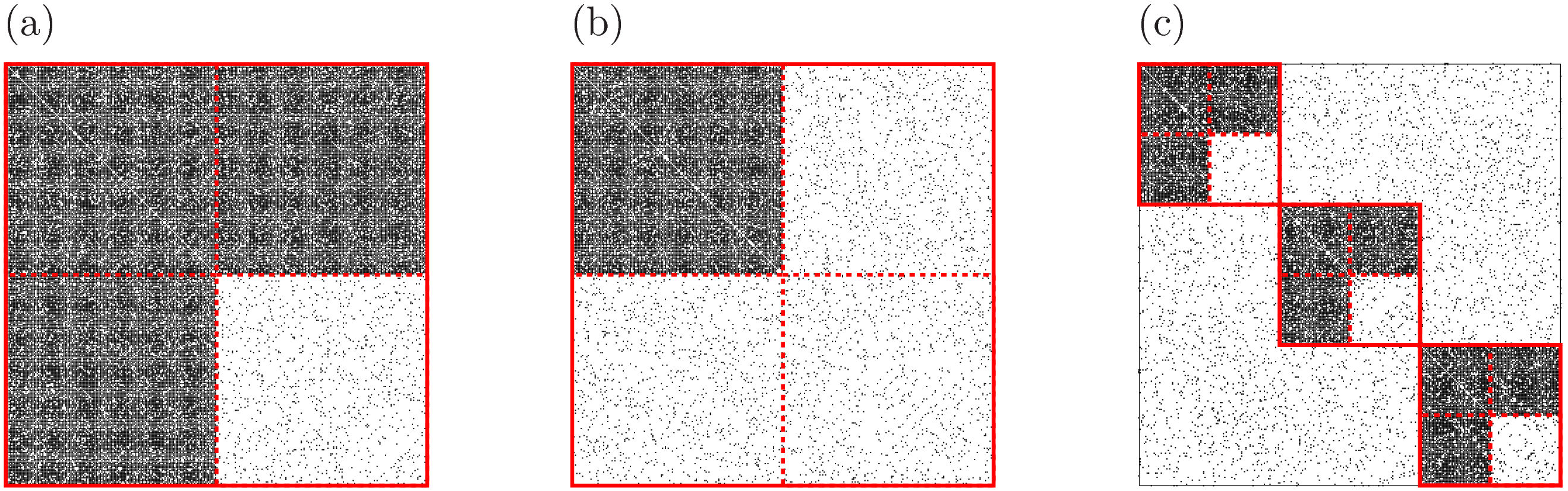
As outlined in Figure 1, a core-periphery structure based on the density of connections is composed of at least a pair of core and periphery blocks. The core block (in the upper left corner of Figs. 1(a) and (b)) has many intra-block connections, whereas, the peripheral block (in the bottom right corner) has relatively few intra-block connections. Connections between core and periphery blocks (in the upper right and bottom left corners) may be abundant (Fig. 1(a)) or not (Fig. 1(b)). Networks may consist of a single core-periphery pair (Figs. 1(a) and (b)) or of multiple core-periphery pairs (Fig. 1(c)).
II.3 Core-periphery detection
In order to detect core-periphery structures we use the Borgatti-Everett (BE) [19], MINRES [22, 63] and the Kojaku-Masuda (KM–ER) [58] algorithms. In the following descriptions of the algorithms, we omit the time label to simplify the notation, recalling that all methods take as input a given adjacency matrix .
In the BE algorithm, one considers an idealised single core-periphery pair, in which each core node is adjacent to all core and peripheral nodes, and each peripheral node is not adjacent to any other peripheral nodes. The adjacency matrix for the idealised single core-periphery pair is given by , with
where or if node is a core node or a peripheral node, respectively, and . The BE algorithm seeks by maximising the similarity between and the adjacency matrix of the given network. The MINRES algorithm also seeks by maximising the similarity between and , however ignoring the contribution from connections between the core and the periphery. As such, MINRES allows the core and periphery blocks to be sparsely connected (Fig. 1(b)). Note that both BE and MINRES algorithms identify only one pair of core and periphery in a given network.
The KM–ER algorithm instead allows multiple core-periphery pairs (Fig. 1(c)). KM–ER considers a network composed of non-overlapping idealised core-periphery pairs, in which there is no connection between different core-periphery pairs. The adjacency matrix for the idealised core-periphery structure is given by , with
where is the index of the core-periphery pair to which node belongs, is Kronecker’s delta, and . The KM–ER algorithm seeks and by maximising
| (5) |
where is the overall density of the network:
| (6) |
In eq. (5), the term accounts for the number of connections that appear in both and , whereas, the term represents the number of edges for the Erdős-Rényi random graph that has the same number of edges as the given network. A large value indicates that the given network has strong core-periphery structure as compared to the Erdős-Rényi random graph.
To maximise , the KM–ER algorithm proceeds as follows [58]. First, we assign each node to a different core, i.e., and for . Then, we reassign the label to each node in a random order as follows. For node , we tentatively assign it to the core of the core-periphery pair to which a neighbour belongs, i.e., we set and . Then, we tentatively assign node to the periphery of the core-periphery pair, i.e., we set and . We repeat this procedure for each neighbour of node and adopt the tentative label— or —that yields the largest increment in . If no relabelling increases , no update of is done. After sweeping all nodes, we end the relabelling procedure if we have not changed any label in the current sweep. Otherwise, we sweep all nodes again in a new random order and repeat the procedure. We run this algorithm ten times starting from the same initial labels (i.e., and ) and adopt the result giving the largest value.
II.3.1 Significance of a core-periphery pair
In order to estimate the significance of the detected core-periphery pairs, we use the statistical method described in Boyd et al., [21], Kojaku and Masuda, [58]. Suppose a single core-periphery pair, described by , is detected by an algorithm—say BE. First, we compute the quality of the core-periphery pair as
| (7) |
Second, we generate randomized Erdős-Rényi random networks, each with the same number of nodes and edges of the original network; for each randomised network , we detect a single core-periphery pair using BE, and compute its quality . Finally, we deem that the original core-periphery pair is significant if it has a larger quality than a fraction of the single core-periphery pairs detected in the randomised networks, where is the significance level. If instead there are multiple core-periphery pairs detected, we apply the aforementioned statistical test to each of them. We suppress the false positives owing to multiple comparisons using the Šidák correction [68], i.e., , where is the targeted significance level. In the following, we refer to banks belonging to insignificant core-periphery pairs as residual banks.
II.3.2 Characterisation of a core-periphery pair
We use the density of connections to quantitatively characterise each block of a core-periphery pair. For the -th core-periphery pair, i.e., including nodes with , we define , and as the fraction of edges within the core block, that between the core and periphery blocks, and that within the periphery block, respectively. These quantities are given by:
| (8) | ||||
| (9) | ||||
| (10) |
where and are the number of nodes of the core and periphery in the th core-periphery pair, respectively.
III Results
III.1 Static network
We start by analysing the static network, which is obtained by setting equal to the entire time span of the dataset. By definition, the BE and MINRES algorithms identify a single core-periphery pair (Figs. 2(a) and 2(b)). In contrast, the KM–ER algorithm identifies four core-periphery pairs (Fig. 2(c)). In this case, the largest and second largest core-periphery pairs mostly consist of Italian and foreign banks, respectively. Thus, the KM–ER algorithm discerns the network behaviour of Italian and foreign banks in an unsupervised way, which is consistent with previous studies [41].

Table 1 reports values of connection density for the core-periphery blocks detected by the three algorithms. In all cases, except for star structure with only one core node, core-periphery pairs satisfy , where is the overall density of the network. This means that the core-periphery characterisation of the network is rather marked for such a long aggregation period.
| BE | 1 | 74 | 276 | 0.98 | 0.50 | 0.11 |
| MINRES | 1 | 122 | 228 | 0.92 | 0.31 | 0.06 |
| KM–ER | 1 | 118 | 107 | 0.91 | 0.57 | 0.13 |
| 2 | 28 | 20 | 0.68 | 0.51 | 0.12 | |
| 3 | 1 | 3 | 0 | 1 | 0 | |
| 4 | 1 | 2 | 0 | 1 | 0 |
III.2 Temporal network
We now move to the analysis of temporal networks, in which is set equal to either a quarter, a month, a week and a day. Figure 3 shows how core-periphery structures detected by the three algorithms change over time, in the case of quarterly networks (refer to Figs. A.7–A.9 for the case of monthly networks).22 2 Shorter time scales cannot be properly shown with these kinds of plots, but their properties will be as well analysed in the following. We see that the KM–ER algorithm detects, almost always, a significantly large core-periphery pair (which we will refer to as main core-periphery pair), accompanied by a few small core-periphery pairs. These small pairs are very short-lived, as they persist for only a few quarters. Remarkably, the number of small core-periphery pairs increases until the beginning of the global financial crisis, and then starts decreasing. Thus, the crisis event marks a tipping point in the tiered organisation of the interbank market. Additionally, the size of the main periphery decreases in time, indicating that main peripheral banks had an increasing tendency to move to small core-periphery pairs (or to become residual). Note also that, similarly to the static network case, for temporal networks the main core-periphery pair detected by the KM–ER algorithm mainly consists of Italian banks (Fig. 4). The second largest pair consists mainly of foreign banks, but this feature emerges only between 2002 and 2009 and for data aggregation periods that are not too short.


To further inspect the effect of the crisis on eMID, we compute the Jaccard’s coefficient for the bank composition of the main core at each pair of time points and , i.e., , where is the set of core nodes of the main core-periphery pair at time . The Jaccard index is large if the cores at times and have many banks in common, and small otherwise. As shown in Figure 5, the main cores detected by all three algorithms experience an abrupt change around 2002 (supposedly after the dot.com bubble burst) and especially in 2008, in the midst of the global financial crisis.

We conclude our analysis by studying the internal structure of the main core-periphery pairs detected by the three algorithms. To this end, we compute the fraction of edges (i.e., the edge density) within the core, that between the core and periphery, and that within the periphery in the main core-periphery pair. Figure 6 shows the density the of different types of edges within the main core-periphery pairs. In most cases, we observe a marked decay in the density of intra-core edges after 2008, leading to a higher segregation of the network. Concerning the specifics of the algorithms, BE and MINRES always return a “standard” core-periphery structure, namely (the less clear case of BE on daily networks will be discussed shortly). The KM–ER algorithm instead returns a more composite picture. For long aggregation periods (i.e., quarterly and monthly), a standard core-periphery structure is detected only before the crisis. Afterwards, we observe : connections between core and periphery become more abundant than those within the core. This is a signature of bipartitivity, and again the structural transition happens during the crisis. For short aggregation periods (weekly and daily), bipartitivity is detected in the majority of cases, in accordance with the findings of Barucca and Lillo, [13].
Finally, focusing on daily networks (which are the noisiest due to the scarcity of connections), bipartite-like structures are detected by the BE, MINRES and KM–ER algorithms in approximately , and of the cases, respectively.

IV Discussion and Conclusions
In this work we employed the KM–ER algorithm [58] to characterise the internal organisation of the electronic market for interbank deposit eMID. As compared to other core-periphery detection algorithms, the KM–ER method stands out by identifying multiple core-periphery pairs allowing, for instance, to discern Italian and foreign banks in an unsupervised way. Note that although KM–ER is designed to detect core-periphery structures, the method has also been able to reveal the bipartite-like organisation of the market. This result is consistent with previous studies [12, 13], in which bipartite-like structures in the eMID network were detected using stochastic block-modelling and its degree-corrected version [56]. In particular, using standard stochastic block-modelling Barucca and Lillo, [12], Barucca and Lillo, [13] found a single core-periphery pair which turned into a bipartite structure for short data aggregation periods, whereas, using degree-corrected stochastic block-modelling bipartitivity emerged also for longer periods. Here we found bipartite-like blocks in the networks by allowing multiple core-periphery pairs without discounting the effect of nodes’ degree, and yet we detected bipartitivity for long data aggregation periods as well. Concerning the temporal evolution of the market, the KM–ER algorithm revealed a structural transition during the global financial crisis, both in terms of network segregation and organisation: the multiplicity of core-periphery pairs disappeared, and the main core-periphery structure was replaced by a bipartite-like structure.
Clearly, the network patterns revealed by any algorithm-based analysis do depend on how the algorithm is designed. It would be useful to perform, in the future, an extensive comparison of the results obtained by both core-periphery and block-model based methods, in order to reveal the market features which are invariant from the observation lens used in the analysis.
Acknowledgements
G.C. and G.C. acknowledge support from the EU projects DOLFINS (640772), CoeGSS (676547), Shakermaker (687941), and SoBigData (654024). N.M. acknowledges the support provided through JST CREST Grant Number JPMJCR1304 and the JST ERATO Grant Number JPMJER1201, Japan. The funders had no role in study design, data collection and analysis, decision to publish, or preparation of the manuscript.
Declarations of Interest
The authors report no conflicts of interest. The authors alone are responsible for the content and writing of the paper.
References
- [1] Acemoglu, D., Ozdaglar, A., and Tahbaz-Salehi, A. (2015). Systemic risk and stability in financial networks. American Economic Review, 105(2):564–608.
- [2] Acharya, V. V. and Merrouche, O. (2013). Precautionary hoarding of liquidity and interbank markets: Evidence from the subprime crisis. Review of Finance, 17(1):107–160.
- [3] Adrian, T. and Shin, H. S. (2010). Liquidity and leverage. Journal of Financial Intermediation, 19(3):418–437.
- [4] Allen, F. and Gale, D. (2000). Financial contagion. Journal of Political Economy, 108(1):1–33.
- [5] Allen, F., Hryckiewicz, A., Kowalewski, O., and Tümer-Alkan, G. (2014). Transmission of financial shocks in loan and deposit markets: Role of interbank borrowing and market monitoring. Journal of Financial Stability, 15:112–126.
- [6] Amini, H., Cont, R., and Minca, A. (2016). Resilience to contagion in financial networks. Mathematical Finance, 26(2):329–365.
- [7] Anand, K., Craig, B., and von Peter, G. (2015). Filling in the blanks: Network structure and interbank contagion. Quantitative Finance, 15(4):625–636.
- [8] Anand, K., van Lelyveld, I., Banai, A., Christiano Silva, T., Friedrich, S., Garratt, R., Halaj, G., Hansen, I., Howell, B., Lee, H., Martínez Jaramillo, S., Molina-Borboa, J., Nobili, S., Rajan, S., Rubens Stancato de Souza, S., Salakhova, D., and Silvestri, L. (2017). The missing links: A global study on uncovering financial network structure from partial data. Journal of Financial Stability, (in press).
- [9] Angelini, P., Nobili, A., and Picillo, C. (2011). The interbank market after august 2007: What has changed, and why? Journal of Money, Credit and Banking, 43(5):923–958.
- [10] Bardoscia, M., Battiston, S., Caccioli, F., and Caldarelli, G. (2015). Debtrank: A microscopic foundation for shock propagation. PLoS ONE, 10(6):e0130406.
- [11] Bardoscia, M., Battiston, S., Caccioli, F., and Caldarelli, G. (2017). Pathways towards instability in financial networks. Nature Communications, 8:14416.
- [12] Barucca, P. and Lillo, F. (2016). Disentangling bipartite and core-periphery structure in financial networks. Chaos, Solitons and Fractals, 88:244–253.
- [13] Barucca, P. and Lillo, F. (2018). The organization of the interbank network and how ecb unconventional measures affected the e-mid overnight market. Computational Management Science, 15(1):33–53.
- [14] Battiston, S., Farmer, J. D., Flache, A., Garlaschelli, D., Haldane, A. G., Heesterbeek, H., Hommes, C., Jaeger, C., May, R., and Scheffer, M. (2016). Complexity theory and financial regulation. Science, 351(6275):818–819.
- [15] Battiston, S., Puliga, M., Kaushik, R., Tasca, P., and Caldarelli, G. (2012). Debtrank: Too central to fail? financial networks, the fed and systemic risk. Scientific Reports, 2:541.
- [16] Beaupain, R. and Durré, A. (2008). The interday and intraday patterns of the overnight market: Evidence from an electronic platform. ECB Working Paper Series 0988.
- [17] Bech, M. L. and Atalay, E. (2010). The topology of the federal funds market. Physica A: Statistical Mechanics and its Applications, 389(22):5223–5246.
- [18] Berrospide, J. M. (2013). Bank liquidity hoarding and the financial crisis: An empirical evaluation. Finance and Economics Discussion Series 03, Board of Governors of the Federal Reserve System (U.S.).
- [19] Borgatti, S. P. and Everett, M. G. (2000). Models of core/periphery structures. Social Networks, 21(4):375–395.
- [20] Boss, M., Elsinger, H., Summer, M., and Thurner, S. (2004). Network topology of the interbank market. Quantitative Finance, 4(6):677–684.
- [21] Boyd, J. P., Fitzgerald, W. J., and Beck, R. J. (2006). Computing core/periphery structures and permutation tests for social relations data. Social Networks, 28(2):165–178.
- [22] Boyd, J. P., Fitzgerald, W. J., Mahutga, M. C., and Smith, D. A. (2010). Computing continuous core/periphery structures for social relations data with minres/svd. Social Networks, 32(2):125–137.
- [23] Brunnermeier, M. K. (2009). Deciphering the liquidity and credit crunch 2007-2008. Journal of Economic Perspectives, 23(1):77–100.
- [24] Caccioli, F., Shrestha, M., Moore, C., and Farmer, J. D. (2014). Stability analysis of financial contagion due to overlapping portfolios. Journal of Banking and Finance, 46:233–245.
- [25] Carreño, J. G. and Cifuentes, R. (2017). Identifying complex core-periphery structures in the interbank market. Journal of Network Theory in Finance, 3(4):49–75.
- [26] Chan-Lau, J. A., Espinosa, M., Giesecke, K., and Solé, J. A. (2009). Assessing the systemic implications of financial linkages. Technical report, IMF Global Financial Stability Report.
- [27] Cifuentes, R., Ferrucci, G., and Shin, H. S. (2005). Liquidity risk and contagion. Journal of the European Economic Association, 3(2/3):556–566.
- [28] Cimini, G. and Serri, M. (2016). Entangling credit and funding shocks in interbank markets. PLoS ONE, 11(8):e0161642.
- [29] Cimini, G., Squartini, T., Gabrielli, A., and Garlaschelli, D. (2015a). Estimating topological properties of weighted networks from limited information. Physical Review E, 92:040802.
- [30] Cimini, G., Squartini, T., Garlaschelli, D., and Gabrielli, A. (2015b). Systemic risk analysis on reconstructed economic and financial networks. Scientific Reports, 5:15758.
- [31] Cocco, J. F., Gomes, F. J., and Martins, N. C. (2009). Lending relationships in the interbank market. Journal of Financial Intermediation, 18(1):24–48.
- [32] Cont, R., Moussa, A., and Santos, E. B. (2013). Network structure and systemic risk in banking systems, pages 327–368. Cambridge University Press.
- [33] Cont, R. and Wagalath, L. (2016). Fire sales forensics: Measuring endogenous risk. Mathematical Finance, 26(4):835–866.
- [34] Craig, B. and Von Peter, G. (2014). Interbank tiering and money center banks. Journal of Financial Intermediation, 23(3):322–347.
- [35] De Masi, G., Iori, G., and Caldarelli, G. (2006). Fitness model for the italian interbank money market. Physical Review E, 74:066112.
- [36] Di Gangi, D., Lillo, F., and Pirino, D. (2015). Assessing systemic risk due to fire sales spillover through maximum entropy network reconstruction. available at https://arxiv.org/abs/1509.00607.
- [37] Diamond, D. W. and Rajan, R. G. (2009). Fear of fire sales and the credit freeze. Working Paper 14925, National Bureau of Economic Research.
- [38] Elsinger, H., Lehar, A., and Summer, M. (2006). Risk assessment for banking systems. Management Science, 52(9):1301–1314.
- [39] Finger, K., Fricke, D., and Lux, T. (2013). Network analysis of the e-mid overnight money market: The informational value of different aggregation levels for intrinsic dynamic processes. Computational Management Science, 10(2):187–211.
- [40] Freixas, X., Parigi, B. M., and Rochet, J.-C. (2000). Systemic risk, interbank relations, and liquidity provision by the central bank. Journal of Money, Credit and Banking, 32(3):611–638.
- [41] Fricke, D. and Lux, T. (2015). Core-periphery structure in the overnight money market: Evidence from the e-mid trading platform. Computational Economics, 45(3):359–395.
- [42] Furfine, C. H. (2003). Interbank exposures: Quantifying the risk of contagion. Journal of Money, Credit and Banking, 35(1):111–128.
- [43] Gai, P., Haldane, A., and Kapadia, S. (2011). Complexity, concentration and contagion. Journal of Monetary Economics, 58(5):453–470.
- [44] Gai, P. and Kapadia, S. (2010). Contagion in financial networks. Proceedings of the Royal Society of London A, 466(2120):2401–2423.
- [45] Gale, D. and Yorulmazer, T. (2013). Liquidity hoarding. Theoretical Economics, 8(2):291–324.
- [46] Gandy, A. and Veraart, L. A. (2016). A bayesian methodology for systemic risk assessment in financial networks. Management Science (articles in advances), pages 1–20.
- [47] Georg, C.-P. (2013). The effect of the interbank network structure on contagion and common shocks. Journal of Banking and Finance, 37(7):2216–2228.
- [48] Glasserman, P. and Young, H. P. (2015). How likely is contagion in financial networks? Journal of Banking and Finance, 50:383–399.
- [49] Greenwood, R., Landier, A., and Thesmar, D. (2015). Vulnerable banks. Journal of Financial Economics, 115(3):471–485.
- [50] Gualdi, S., Cimini, G., Primicerio, K., Clemente, R. D., and Challet, D. (2016). Statistically validated network of portfolio overlaps and systemic risk. Scientific Reports, 6:39467.
- [51] Haldane, A. G. and May, R. M. (2011). Systemic risk in banking ecosystems. Nature, 469:351–355.
- [52] Hüser, A.-C. (2015). Too interconnected to fail: A survey of the interbank networks literature. Journal of Network Theory In Finance, 1(3):1–50.
- [53] Iori, G., Jafarey, S., and Padilla, F. G. (2006). Systemic risk on the interbank market. Journal of Economic Behavior and Organization, 61(4):525–542.
- [54] Iori, G., Mantegna, R. N., Marotta, L., Miccichè, S., Porter, J., and Tumminello, M. (2015). Networked relationships in the e-mid interbank market: A trading model with memory. Journal of Economic Dynamics and Control, 50:98–116.
- [55] Iori, G., Masi, G. D., Precup, O. V., Gabbi, G., and Caldarelli, G. (2008). A network analysis of the italian overnight money market. Journal of Economic Dynamics and Control, 32(1):259–278.
- [56] Karrer, B. and Newman, M. E. J. (2011). Stochastic blockmodels and community structure in networks. Physical Review E, 83:016107.
- [57] Kaufman, G. G. (1994). Bank contagion: A review of the theory and evidence. Journal of Financial Services Research, 8(2):123–150.
- [58] Kojaku, S. and Masuda, N. (2017). Finding multiple core-periphery pairs in networks. Physical Review E, 96:052313.
- [59] Krause, A. and Giansante, S. (2012). Interbank lending and the spread of bank failures: A network model of systemic risk. Journal of Economic Behavior and Organization, 83(3):583–608.
- [60] Langfield, S., Liu, Z., and Ota, T. (2014). Mapping the uk interbank system. Journal of Banking and Finance, 45:288–303.
- [61] Lee, S. H. (2013). Systemic liquidity shortages and interbank network structures. Journal of Financial Stability, 9(1):1–12.
- [62] León, C. and Berndsen, R. J. (2014). Rethinking financial stability: Challenges arising from financial networks’ modular scale-free architecture. Journal of Financial Stability, 15:241–256.
- [63] Lip, S. Z. (2011). A fast algorithm for the discrete core/periphery bipartitioning problem. available at https://arxiv.org/abs/1102.5511.
- [64] Martinez-Jaramillo, S., Alexandrova-Kabadjova, B., Bravo-Benitez, B., and Solórzano-Margain, J. P. (2014). An empirical study of the mexican banking system’2 network and its implications for systemic risk. Journal of Economic Dynamics and Control, 40:242–265.
- [65] Nier, E. W., Yang, J., Yorulmazer, T., and Alentorn, A. (2007). Network models and financial stability. Journal of Economic Dynamics and Control, 31(6):2033–2060.
- [66] Rochet, J.-C. and Tirole, J. (1996). Interbank lending and systemic risk. Journal of Money, Credit and Banking, 28(4):733–762.
- [67] Serri, M., Caldarelli, G., and Cimini, G. (2017). How the interbank market becomes systemically dangerous: an agent-based network model of financial distress propagation. Journal of Network Theory in Finance, 3(1):1–15.
- [68] Šidák, Z. (1967). Rectangular confidence regions for the means of multivariate normal distributions. Journal of the American Statistical Association, 62(318):626–633.
- [69] Silva, T. C., de Souza, S. R. S., and Tabak, B. M. (2016). Network structure analysis of the brazilian interbank market. Emerging Markets Review, 26:130–152.
- [70] Soramäki, K., Bech, M. L., Arnold, J., Glass, R. J., and Beyeler, W. E. (2007). The topology of interbank payment flows. Physica A: Statistical Mechanics and its Applications, 379(1):317–333.
- [71] Squartini, T., Almog, A., Caldarelli, G., van Lelyveld, I., Garlaschelli, D., and Cimini, G. (2017). Enhanced capital-asset pricing model for the reconstruction of bipartite financial networks. Physical Review E, 96:032315.
- [72] Veld, D. i. t. and van Lelyveld, I. (2014). Finding the core: Network structure in interbank markets. Journal of Banking and Finance, 49:27–40.
- [73] Verma, T., Russmann, F., Araújo, N., Nagler, J., and Herrmann, H. (2016). Emergence of core-peripheries in networks. Nature Communications, 7:10441.


