跳到论文正文
W Papers独立论文阅读器 arXiv:1802.04963 论文正文 计算阅读时间 · 0%
引用这篇论文根据当前论文元数据生成,正式投稿前建议核对。


License: arXiv.org perpetual non-exclusive license
arXiv:1802.04963v3 [math.NA] 07 Oct 2019

∎

Superconvergent recovery of Raviart–Thomas mixed finite elements on triangular grids

Randolph E. Bank    Yuwen Li Affiliation: R. E. Bank: Department of Mathematics, University of California, San Diego, La Jolla, California 92093-0112.  Email:rbank@ucsd.edu
Y. Li: Department of Mathematics, University of California, San Diego, La Jolla, California 92093-0112.  Email:yul739@ucsd.edu
Received: April 4, 2019 / Accepted: date
Abstract

For the second lowest order Raviart–Thomas mixed method, we prove that the canonical interpolant and finite element solution for the vector variable in elliptic problems are superclose in the H⁡(div)H(\divg)-norm on mildly structured meshes, where most pairs of adjacent triangles form approximate parallelograms. We then develop a family of postprocessing operators for Raviart–Thomas mixed elements on triangular grids by using the idea of local least squares fittings. Super-approximation property of the postprocessing operators for the lowest and second lowest order Raviart–Thomas elements is proved under mild conditions. Combining the supercloseness and super-approximation results, we prove that the postprocessed solution superconverges to the exact solution in the L2L^{2}-norm on mildly structured meshes.

Keywords: 
superconvergence, mildly structured grids, mixed methods, Raviart–Thomas elements, second order elliptic equations
MSC
65N30, 65N50

1 Introduction and preliminaries

Gradient recovery methods for Lagrange elements have been studied extensively by many authors, see, e.g., [30, 29, 3, 4, 5, 27, 28, 26] and references therein. Let uu be the exact solution of Poisson’s equation and uhu_{h} be the finite element solution from Lagrange elements. In general ∇uh\nabla u_{h} rather than uhu_{h} is the main quantity of interest. Gradient recovery methods aim to get a new approximation 𝒑h\bm{p}_{h} to ∇u\nabla u by postprocessing uhu_{h} or ∇uh\nabla u_{h}. Comparing to ∇uh\nabla u_{h}, 𝒑h\bm{p}_{h} is often H1H^{1}-conforming and 𝒑h\bm{p}_{h} superconverges to ∇u\nabla u in some situation. In addition, 𝒑h\bm{p}_{h} can be used to develop a posteriori error estimators. The recovery-based a posteriori error estimators are popular for their simplicity and asymptotic exactness, see, e.g., [29, 4, 27].

To derive recovery-type superconvergence, a common ingredient is the so-called supercloseness estimate showing that the canonical interpolant and finite element solution are superclose in some norm. In this paper, we consider the second lowest order Raviart–Thomas (denoted by R​T1RT_{1}) mixed method for the second order elliptic equation, namely, (1.5) with r=1r=1. We shall prove that the canonical interpolant Πh1​𝒑\Pi_{h}^{1}\bm{p} and the finite element solution 𝒑h1\bm{p}_{h}^{1} are superclose in the H⁡(div)H(\divg)-norm under mildly structured grids, i.e., most pairs of adjacent triangles in grids form O⁡(h1+α)O(h^{1+\alpha})-approximate parallelograms except for a region with measure O⁡(hβ)O(h^{\beta}), see Definitions 2.1 and 2.2. The supercloseness result in this paper generalizes a result for the R​T0RT_{0} mixed method in [19]. For Poisson’s equation, Brandts [7] proved a supercloseness estimate for R​T1RT_{1} on three-line grids, i.e., each edge in grids is parallel to one of three fixed lines.

To relax the restriction on mesh structures in supercloseness analysis, we give a constructive proof for Theorem 3.2 instead of using the odd-even argument and the Bramble–Hilbert lemma employed in [6, 7]. For Lagrange elements over (α,β)(\alpha,\beta)-grids, the authors in [3] transferred the local error ∫T∇(u−uI)⋅∇vh\int_{T}\nabla(u-u_{I})\cdot\nabla v_{h} on each element TT to line integrals using the divergence theorem, where uIu_{I} is the linear Lagrange interpolant. Then line integrals are grouped in terms of tangential components of ∇vh\nabla v_{h} by delicate triangular integral identities. However, it’s not clear how to handle the local error ∫T(𝒑−Πhr​𝒑)⋅𝒒h\int_{T}(\bm{p}-\Pi_{h}^{r}\bm{p})\cdot\bm{q}_{h} for the R​TrRT_{r} element in a similar fashion. Our key observation is that R​TrRT_{r} elements satisfy the divergence-free property, i.e., div⁡(𝒑r+1−Πhr​𝒑r+1)=0\divg(\bm{p}_{r+1}-\Pi_{h}^{r}\bm{p}_{r+1})=0 on each triangle TT provided 𝒑r+1∈𝒫r+1​(T)2\bm{p}_{r+1}\in\mathcal{P}_{r+1}(T)^{2}. Hence 𝒑r+1−Πhr​𝒑r+1=∇⟂wr+2\bm{p}_{r+1}-\Pi_{h}^{r}\bm{p}_{r+1}=\nabla^{\perp}w_{r+2} for some wr+2∈𝒫r+2​(T)w_{r+2}\in\mathcal{P}_{r+2}(T) and it can be handled by Green’s theorem, see Section 5.

For mixed methods, the finite element solution 𝒑h\bm{p}_{h} approximating the vector variable 𝒑∈H⁡(div,Ω)\bm{p}\in H(\divg,\Omega) is the main quantity of physical interest. As far as we know, existing postprocessing/recovery techniques for 𝒑\bm{p} and 𝒑h\bm{p}_{h} are restricted to strongly structured grids, e.g., three-line, translation invariant and rectangular grids, see, e.g., [11, 14, 13, 7]. As grids become increasingly unstructured, the rate of superconvergence of ‖𝒑−Kh​Πh​𝒑‖0,Ω\|\bm{p}-K_{h}\Pi_{h}\bm{p}\|_{0,\Omega} deteriorates, where Πh\Pi_{h} is the canonical interpolation and KhK_{h} is some postprocessing operator. In addition, most of the existing results of recovery methods focus on the lowest order case while the analysis of recovery operators for higher order elements is limited, especially on irregular grids. In this paper, we construct a new family of recovery operators RhrR_{h}^{r} for R​TrRT_{r} (r≥0r\geq 0) elements by fitting the numerical solution 𝒑h\bm{p}_{h} with a vector polynomial of degree r+1r+1 in the least squares(LS) sense on each local patch surrounding each vertex in triangular grids. We shall show that Rh0R_{h}^{0} and Rh1R_{h}^{1} have nice super-approximation property under mild and easy-to-check conditions. The order of approximation of RhrR_{h}^{r} is almost independent of the mesh structure. Combining the supercloseness and RhrR_{h}^{r}, we finally obtain the superconvergence of the postprocessed R​T0RT_{0} and R​T1RT_{1} solutions to the exact solution, see Theorem 4.4.

Recovery by local least squares fitting is not a new idea. The famous Zienkiewicz–Zhu(ZZ) superconvergent patch recovery GhG_{h} is based on it, see, e.g., [30, 29]. For linear elements, ∥∇u−Gh∇u∥=O(h2)\|\nabla u-G_{h}\nabla u\|=O(h^{2}) under strongly regular grids (see [17]), that is, each pair of adjacent triangles form an O⁡(h2)O(h^{2}) approximate parallelogram. Alternatively, Zhang and Naga [28] proposed a different LS-based patch recovery operator GhrG_{h}^{r} for Lagrange elements of degree rr by postprocessing the scalar function uu rather than ∇u\nabla u. Roughly speaking, ‖∇u−Ghr​u‖=O⁡(hr+1)\|\nabla u-G_{h}^{r}u\|=O(h^{r+1}) provided each LS problem has a unique solution on each local patch. RhrR_{h}^{r} can be viewed as a Raviart–Thomas version of Ghr+1G_{h}^{r+1}. In practice, the excellent superconvergence property of GhrG_{h}^{r} is attributed to the unique solvability of vertex-based LS problems, which is difficult to prove on unstructured grids. For example, [22] is mainly devoted to the analysis of the uniqueness of the LS solution for Gh1G_{h}^{1} on unstructured grids. As far as we know, there is no similar analysis for GhrG_{h}^{r} with r≥2r\geq 2. We shall give a practical criterion of uniqueness for Gh2G_{h}^{2} on unstructured grids, which also works for Rh1R_{h}^{1}, see Theorem 4.1.

In this paper, we consider the second order elliptic equation

−div(a2(𝒙)∇u+𝒂1(𝒙)u)+a0(𝒙)u\displaystyle-\divg(a_{2}(\bm{x})\nabla u+\bm{a}_{1}(\bm{x})u)+a_{0}(\bm{x})u =f⁡(𝒙),𝒙∈Ω,\displaystyle=f(\bm{x}),\quad\bm{x}\in\Omega, (1.1a)
u\displaystyle u =g⁡(𝒙),𝒙∈∂Ω,\displaystyle=g(\bm{x}),\quad\bm{x}\in\partial\Omega, (1.1b)

where div=∇⋅\divg=\nabla\cdot is the divergence operator, a2,a0a_{2},a_{0} are scalar-valued and 𝒂1\bm{a}_{1} is vector-valued, Ω⊂ℝ2\Omega\subset\mathbb{R}^{2} is a bounded and simply-connected Lipschitz domain. Assume that a2,𝒂1,a0a_{2},\bm{a}_{1},a_{0} are sufficiently smooth on Ω¯\overline{\Omega} and a2≥Λ>0a_{2}\geq\Lambda>0 for some constant Λ.\Lambda. Let

𝒑\displaystyle\bm{p} =a2∇u+𝒂1u,\displaystyle=a_{2}\nabla u+\bm{a}_{1}u,
a\displaystyle a =a2−1,𝒃=a2−1𝒂1,c=a0.\displaystyle=a_{2}^{-1},\quad\bm{b}=a_{2}^{-1}\bm{a}_{1},\quad c=a_{0}.

Equation (1.1) is equivalent to the first order system

a​𝒑−𝒃​u−∇u\displaystyle a\bm{p}-\bm{b}u-\nabla u =0,𝒙∈Ω,\displaystyle=0,\quad\bm{x}\in\Omega, (1.2a)
−div⁡𝒑+c​u\displaystyle-\divg\bm{p}+cu =f,𝒙∈Ω,\displaystyle=f,\quad\bm{x}\in\Omega, (1.2b)
u\displaystyle u =g,𝒙∈∂Ω.\displaystyle=g,\quad\bm{x}\in\partial\Omega. (1.2c)

Let 𝒬=H⁡(div,Ω):={𝒒∈L2​(Ω)2:div⁡𝒒∈L2​(Ω)}\mathcal{Q}=H(\divg,\Omega):=\{\bm{q}\in L^{2}(\Omega)^{2}:\divg\bm{q}\in L^{2}(\Omega)\} and 𝒱=L2​(Ω).\mathcal{V}=L^{2}(\Omega). The mixed formulation for (1.2) is to find the pair {𝒑,u}∈𝒬×𝒱\{\bm{p},u\}\in\mathcal{Q}\times\mathcal{V}, such that

(a​𝒑,𝒒)−(𝒒,𝒃​u)+(div⁡𝒒,u)\displaystyle(a\bm{p},\bm{q})-(\bm{q},\bm{b}u)+(\divg\bm{q},u) =⟨𝒒⋅𝒏,g⟩,\displaystyle=\langle\bm{q}\cdot\bm{n},g\rangle, (1.3a)
−(div⁡𝒑,v)+(c​u,v)\displaystyle-(\divg\bm{p},v)+(cu,v) =(f,v),\displaystyle=(f,v), (1.3b)

for each pair {𝒒,v}∈𝒬×𝒱\{\bm{q},v\}\in\mathcal{Q}\times\mathcal{V}. Here ⟨⋅,⋅⟩\langle\cdot,\cdot\rangle denotes the L2L^{2}-inner product on ∂Ω.\partial\Omega.

Let 𝒯h\mathcal{T}_{h} be a collection of triangles that forms a triangulation of Ω.\Omega. Let hT=|T|12h_{T}=|T|^{\frac{1}{2}} be the diameter of TT, where |T||T| is the area of TT. Let h=maxT∈𝒯h⁡hT<1h=\max_{T\in\mathcal{T}_{h}}h_{T}<1 be the mesh-size. 𝒯h\mathcal{T}_{h} is assumed to quasi-uniform, namely, maxT∈𝒯h⁡hT≤C0​(minT∈𝒯h⁡hT)\max_{T\in\mathcal{T}_{h}}h_{T}\leq C_{0}(\min_{T\in\mathcal{T}_{h}}h_{T}) for some generic constant C0C_{0}. The quasi-uniformity implies the minimum angle condition (MAC), namely, there exists a fixed constant Θ>0\Theta>0, such that θ≥Θ>0\theta\geq\Theta>0 for any angle θ\theta of any triangle T∈𝒯hT\in\mathcal{T}_{h}. Given a one-dimensional or two-dimensional subset U⊂ℝ2U\subset\mathbb{R}^{2}, let

𝒫r​(U)={v:v​is a polynomial on ​U​ of degree ≤r}\mathcal{P}_{r}(U)=\{v:v\ \text{is\ a\ polynomial\ on }U\text{ of\ degree }\leq r\}

denote the space of polynomials of degree ≤r.\leq r. Let ℰh,ℰho,ℰh∂\mathcal{E}_{h},\mathcal{E}_{h}^{o},\mathcal{E}_{h}^{\partial} denote the set of edges, interior edges and boundary edges in 𝒯h\mathcal{T}_{h} , respectively. Let 𝒩h\mathcal{N}_{h} denote the set of vertices in 𝒯h\mathcal{T}_{h}. Several kinds of local patches are useful for finite element superconvergence analysis. For 𝒛∈𝒩h,\bm{z}\in\mathcal{N}_{h}, let ωz\omega_{z} be the union of triangles in 𝒯h\mathcal{T}_{h} sharing zz as a vertex. For e∈ℰh,e\in\mathcal{E}_{h}, let ωe\omega_{e} be the union of triangles in 𝒯h\mathcal{T}_{h} sharing ee as an edge. For T∈𝒯h,T\in\mathcal{T}_{h}, let ωT\omega_{T} be the union of TT and triangles in 𝒯h\mathcal{T}_{h} sharing at least one vertex with TT. The local nodes, edges , and triangles in UU are 𝒩h​(U)={z∈𝒩h:z∈U¯}\mathcal{N}_{h}(U)=\{z\in\mathcal{N}_{h}:z\in\bar{U}\}, ℰh​(U)={e∈ℰh:e⊂U¯}\mathcal{E}_{h}(U)=\{e\in\mathcal{E}_{h}:e\subset\bar{U}\}, and 𝒯h​(U)={T∈𝒯h:T⊂U¯}\mathcal{T}_{h}(U)=\{T\in\mathcal{T}_{h}:T\subset\bar{U}\}, respectively.

For r≥0r\geq 0 and T∈𝒯hT\in\mathcal{T}_{h}, define the space of shape functions

ℛ𝒯r(T):={(v1v2)+v3(x1x2):vi∈𝒫r(T),i=1,2,3}.\mathcal{RT}_{r}(T):=\left\{\begin{pmatrix}v_{1}\\ v_{2}\end{pmatrix}+v_{3}\begin{pmatrix}x_{1}\\ x_{2}\end{pmatrix}:v_{i}\in\mathcal{P}_{r}(T),i=1,2,3\right\}. (1.4)

The R​TrRT_{r} finite element spaces are

𝒬hr:={𝒒h∈𝒬:𝒒h|T∈ℛ𝒯r(T),∀T∈𝒯h},\displaystyle\mathcal{Q}_{h}^{r}:=\left\{\bm{q}_{h}\in\mathcal{Q}:\bm{q}_{h}|_{T}\in\mathcal{RT}_{r}(T),\ \forall T\in\mathcal{T}_{h}\right\},
𝒱hr:={vh∈𝒱:vh|T∈𝒫r(T),∀T∈𝒯h}.\displaystyle\mathcal{V}_{h}^{r}:=\{v_{h}\in\mathcal{V}:v_{h}|_{T}\in\mathcal{P}_{r}(T),\ \forall T\in\mathcal{T}_{h}\}.

The mixed method for (1.3) is to find {𝒑hr,uhr}∈𝒬hr×𝒱hr\{\bm{p}_{h}^{r},u_{h}^{r}\}\in\mathcal{Q}_{h}^{r}\times\mathcal{V}_{h}^{r}, such that

(a​𝒑hr,𝒒h)−(𝒒h,𝒃​uhr)+(div⁡𝒒h,uhr)\displaystyle(a\bm{p}_{h}^{r},\bm{q}_{h})-(\bm{q}_{h},\bm{b}u_{h}^{r})+(\divg\bm{q}_{h},u_{h}^{r}) =⟨𝒒h⋅𝒏,g⟩,\displaystyle=\langle\bm{q}_{h}\cdot\bm{n},g\rangle, 𝒒h∈𝒬hr,\displaystyle\quad\bm{q}_{h}\in\mathcal{Q}_{h}^{r}, (1.5a)
−(div⁡𝒑hr,vh)+(c​uh,vh)\displaystyle-(\divg\bm{p}_{h}^{r},v_{h})+(cu_{h},v_{h}) =(f,vh),\displaystyle=(f,v_{h}), vh∈𝒱hr.\displaystyle\quad v_{h}\in\mathcal{V}_{h}^{r}. (1.5b)

Under mild assumptions, Douglas and Roberts [12] proved the well-posedness and a priori error estimates for the method (1.5).

Given a positive integer ss and a sufficiently smooth function vv, let

|Ds​v|:=∑α1+α2=s|∂α1+α2∂x1α1​∂x2α2​v|.|D^{s}v|:=\sum_{\alpha_{1}+\alpha_{2}=s}\left|\frac{\partial^{\alpha_{1}+\alpha_{2}}}{\partial x_{1}^{\alpha_{1}}\partial x_{2}^{\alpha_{2}}}v\right|.

For a domain UU, the Sobolev seminorms and norms are defined by

|v|s,p,U=(∫U|Dsv|p)1p,∥v∥s,p,U=(∑m=0s|v|m,p,Up)1p,\displaystyle|v|_{s,p,U}=\big(\int_{U}|D^{s}v|^{p}\big)^{\frac{1}{p}},\quad\|v\|_{s,p,U}=\big(\sum_{m=0}^{s}|v|_{m,p,U}^{p}\big)^{\frac{1}{p}},
|v|m,U=|v|m,2,U,‖v‖m,U=‖v‖m,2,U,\displaystyle|v|_{m,U}=|v|_{m,2,U},\quad\|v\|_{m,U}=\|v\|_{m,2,U},

Sobolev norms with ∞\infty-index and norms of vector-valued functions are generalized in usual ways.

Let |v|h,m,U:=(∑T∈𝒯h|v|m,T2)12|v|_{h,m,U}:=\big(\sum_{T\in\mathcal{T}_{h}}|v|_{m,T}^{2}\big)^{\frac{1}{2}} denote the mesh-dependent semi-norm w.r.t. 𝒯h\mathcal{T}_{h}. We say A≲BA\lesssim B provided A≤C​B,A\leq CB, where CC is a generic constant that may change from line to line, and depends only on the shape regularity of 𝒯h\mathcal{T}_{h} measured by C0C_{0} or Θ.\Theta. We say A≈BA\approx B if A≲BA\lesssim B and B≲A.B\lesssim A. The regularity condition will be indicated on right hand sides of estimates. In addition to 𝒬hr\mathcal{Q}_{h}^{r} and 𝒱hr\mathcal{V}_{h}^{r}, we need the standard nodal finite element space

𝒲hr={w∈C(Ω):w|T∈𝒫r(T),∀T∈𝒯h},\displaystyle\mathcal{W}_{h}^{r}=\{w\in C(\Omega):w|_{T}\in\mathcal{P}_{r}(T),\ \forall T\in\mathcal{T}_{h}\},

where C⁡(Ω)C(\Omega) is the space of continuous functions on Ω\Omega. We present two well-known inequalities that will be used in the rest of this paper.

Theorem 1.1 (Interpolation error)

Let Ihr:C⁡(Ω)→𝒲hrI_{h}^{r}:C(\Omega)\rightarrow\mathcal{W}_{h}^{r} denote the Lagrange interpolation of degree rr. For T∈𝒯hT\in\mathcal{T}_{h} and r≥1,r\geq 1, it holds that

‖v−Ihr​v‖0,γ,T≲hr+2γ​|v|h,r+1,T,1≤γ≤∞.\|v-I_{h}^{r}v\|_{0,\gamma,T}\lesssim h^{r+\frac{2}{\gamma}}|v|_{h,r+1,T},\quad 1\leq\gamma\leq\infty. (1.6)
Theorem 1.2 (Trace inequalities )

For T∈𝒯hT\in\mathcal{T}_{h} and v∈H1​(T)v\in H^{1}(T), it holds that

‖v‖0,∂T≲hT−12​‖v‖0,T+hT12​‖∇v‖0,T.\displaystyle\|v\|_{0,\partial T}\lesssim h_{T}^{-\frac{1}{2}}\|v\|_{0,T}+h_{T}^{\frac{1}{2}}\|\nabla v\|_{0,T}. (1.7)

2 Local error expansions

Refer to caption
Figure 1: A local triangle TT and associated quantities.

We begin with geometric identities on a local element TT. It has three vertices {zk}k=13\{z_{k}\}_{k=1}^{3}, oriented counterclockwise, and corresponding barycentric coordinates {λk}k=13\{\lambda_{k}\}_{k=1}^{3}. Let eke_{k} denote the edge opposite to zkz_{k}, θk\theta_{k} the angle opposite to eke_{k}, ℓk\ell_{k} the length of eke_{k}, dkd_{k} the distance from zkz_{k} to eke_{k}, 𝒕k\bm{t}_{k} the unit tangent to eke_{k}, oriented counterclockwise, 𝒏k\bm{n}_{k} the unit outward normal to eke_{k}, ∂𝒕k\partial_{\bm{t}_{k}} the tangential derivative, ∂𝒏k\partial_{\bm{n}_{k}} the normal derivative, and ∂𝒕k​𝒏k2\partial^{2}_{\bm{t}_{k}\bm{n}_{k}} the second mixed derivative, see Fig. 1. Corresponding quantities on triangles T′T^{\prime} and T′′T^{\prime\prime} have superscripts ′\prime and ′′\prime\prime respectively. The subscripts are equivalent mod 3, e.g., ℓ4=ℓ1,θ0=θ3.\ell_{4}=\ell_{1},\theta_{0}=\theta_{3}.

We have the rotational gradient ∇⟂v=(−∂x2v,∂x1v)⊺\nabla^{\perp}v=\left(-\partial_{x_{2}}v,\partial_{x_{1}}v\right)^{\intercal}, and the adjoint ∇×𝒒=∂x1q2−∂x2q1.\nabla\times\bm{q}=\partial_{x_{1}}q_{2}-\partial_{x_{2}}q_{1}. ∇⟂\nabla^{\perp} and ∇⁣×\nabla\times are related by Green’s formula

∫T∇⟂w⋅𝒒=∫∂Tw𝒒⋅𝒕−∫Tw∇×𝒒,\int_{T}\nabla^{\perp}w\cdot\bm{q}=\int_{\partial T}w\bm{q}\cdot\bm{t}-\int_{T}w\nabla\times\bm{q}, (2.1)

where 𝒕\bm{t} is the unit tangent to ∂K\partial K oriented counterclockwise. For 𝒗∈ℝ2\bm{v}\in\mathbb{R}^{2}, define 𝒗⟂=(−v2,v1)\bm{v}^{\perp}=(-v_{2},v_{1}). Clearly, 𝒏k⟂=𝒕k,\bm{n}_{k}^{\perp}=\bm{t}_{k}, 𝒕k⟂=−𝒏k.\bm{t}_{k}^{\perp}=-\bm{n}_{k}.

Now we introduce basic definitions for R​TrRT_{r} elements. For e∈ℰh,e\in\mathcal{E}_{h}, let {(wj,𝒈j)}j=1r+1\{(w_{j},\bm{g}_{j})\}_{j=1}^{r+1} denote the Gaussian quadrature rule on ee, where {𝒈j}\{\bm{g}_{j}\} are quadrature points and {wj}\{w_{j}\} are corresponding weights. {(wj,𝒈j)}j=1r+1\{(w_{j},\bm{g}_{j})\}_{j=1}^{r+1} is exact for 𝒫2​r+1​(e)\mathcal{P}_{2r+1}(e), i.e.,

∫ev=|e|​∑j=1r+1wj​v​(𝒈j)​ for all ​v∈𝒫2​r+1​(e),\int_{e}v=|e|\sum_{j=1}^{r+1}w_{j}v(\bm{g}_{j})\text{ for all }v\in\mathcal{P}_{2r+1}(e), (2.2)

where |e||e| is the length of e.e. Let vj∈𝒫r​(e)v_{j}\in\mathcal{P}_{r}(e) be the polynomial that is wj−1w_{j}^{-1} at 𝒈j\bm{g}_{j} and 00 at the rest of quadrature points. For T∈𝒯h,T\in\mathcal{T}_{h}, let {λl}l=1r⁡(r+1)/2\{\lambda_{l}\}_{l=1}^{r(r+1)/2} be the nodal basis function of Lagrange elements of degree r−1r-1 on TT ({λl}=∅\{\lambda_{l}\}=\emptyset if r=0r=0; {λl}={1}\{\lambda_{l}\}=\{1\} if r=1r=1). We can specify degrees of freedom of R​TrRT_{r} elements as

𝒩ej​(𝒒):=1|e|​∫e𝒒⋅𝒏e​vj,𝒩Tl​m​(𝒒):=1|T|​∫Tqm​λl,\mathcal{N}_{e}^{j}(\bm{q}):=\frac{1}{|e|}\int_{e}\bm{q}\cdot\bm{n}_{e}v_{j},\quad\mathcal{N}_{T}^{lm}(\bm{q}):=\frac{1}{|T|}\int_{T}q_{m}\lambda_{l},

where 𝒏e\bm{n}_{e} is a unit normal to ee, 𝒒=(q1,q2)⊺\bm{q}=(q_{1},q_{2})^{\intercal}, and 1≤j≤r+11\leq j\leq r+1, 1≤l≤r(r+1)/2,m=1,2.1\leq l\leq r(r+1)/2,m=1,2. By (2.2) and the definition of vjv_{j}, we have 𝒩ej​(𝒒)=𝒒⁡(𝒈j)⋅𝒏e\mathcal{N}_{e}^{j}(\bm{q})=\bm{q}(\bm{g}_{j})\cdot\bm{n}_{e} provided 𝒒∈𝒫r+1​(e)2\bm{q}\in\mathcal{P}_{r+1}(e)^{2}. For 𝒒∈H1​(Ω)2\bm{q}\in H^{1}(\Omega)^{2}, the R​TrRT_{r} interpolant Πhr​𝒒∈𝒬hr\Pi_{h}^{r}\bm{q}\in\mathcal{Q}_{h}^{r} satisfies

𝒩ej​(Πhr​𝒒)\displaystyle\mathcal{N}_{e}^{j}(\Pi_{h}^{r}\bm{q}) =𝒩ej(𝒒),𝒩Tl​m(Πhr𝒒)=𝒩Tl​m(𝒒),\displaystyle=\mathcal{N}_{e}^{j}(\bm{q}),\quad\mathcal{N}_{T}^{lm}(\Pi_{h}^{r}\bm{q})=\mathcal{N}_{T}^{lm}(\bm{q}),

for all indices j,l,mj,l,m, and e∈ℰh,T∈𝒯he\in\mathcal{E}_{h},T\in\mathcal{T}_{h}. The existence and uniqueness of Πhr​𝒒\Pi_{h}^{r}\bm{q} is always guaranteed. In addition, Πhr\Pi_{h}^{r} is stable in the L∞L^{\infty}-norm

‖Πhk​𝒒‖0,∞,T≲‖𝒒‖0,∞,T,T∈𝒯h.\|\Pi_{h}^{k}\bm{q}\|_{0,\infty,T}\lesssim\|\bm{q}\|_{0,\infty,T},\quad T\in\mathcal{T}_{h}. (2.3)

For v∈𝒱v\in\mathcal{V}, the interpolant Phr​vP_{h}^{r}v is the L2L^{2}-projection of vv onto 𝒱hr\mathcal{V}_{h}^{r}. There is a nice commuting property about PhrP^{r}_{h}, Πhr\Pi^{r}_{h} and div\divg, i.e.,

div⁡(Πhr​𝒒)=Phr​(div⁡𝒒),∀𝒒∈H1​(Ω)2.\divg(\Pi_{h}^{r}\bm{q})=P_{h}^{r}(\divg\bm{q}),\quad\forall\bm{q}\in H^{1}(\Omega)^{2}. (2.4)

The following interpolation error estimates hold, see, e.g., [12].

‖𝒒−Πhr​𝒒‖0,Ω≲hr+1​|𝒒|h,r+1,Ω,\displaystyle\|\bm{q}-\Pi_{h}^{r}\bm{q}\|_{0,\Omega}\lesssim h^{r+1}|\bm{q}|_{h,r+1,\Omega}, (2.5a)
‖div⁡(𝒒−Πhr​𝒒)‖0,Ω≲hr+1​|div⁡𝒒|h,r+1,Ω,\displaystyle\|\divg(\bm{q}-\Pi_{h}^{r}\bm{q})\|_{0,\Omega}\lesssim h^{r+1}|\divg\bm{q}|_{h,r+1,\Omega}, (2.5b)
‖v−Phr​v‖0,Ω≲hr+1​|v|h,r+1,Ω.\displaystyle\|v-P_{h}^{r}v\|_{0,\Omega}\lesssim h^{r+1}|v|_{h,r+1,\Omega}. (2.5c)

In the rest of this section, we will present variational error expansions for the R​T1RT_{1} element. Comparing to R​T0RT_{0}, the theory of R​T1RT_{1} is much more complicated. Let dd be the diameter of the circumscribed circle of TT. For each edge eke_{k}, there are several associated geometric quantities

μ11,k1=15760​(3​ℓk4−3​(ℓk−12−ℓk+12)2−4​ℓk2​(ℓk−12+ℓk+12)),\displaystyle\mu^{1}_{11,k}=\frac{1}{5760}\big(3\ell_{k}^{4}-3(\ell_{k-1}^{2}-\ell_{k+1}^{2})^{2}-4\ell_{k}^{2}(\ell_{k-1}^{2}+\ell_{k+1}^{2})\big),
μ112,k=μ121,k=11440​dℓ1ℓ2ℓ3(ℓk−12−ℓk+12),μ122,k=−11440​d2ℓ12ℓ22ℓ32,\displaystyle\mu^{1}_{12,k}=\mu^{1}_{21,k}=\frac{1}{1440d}\ell_{1}\ell_{2}\ell_{3}(\ell_{k-1}^{2}-\ell_{k+1}^{2}),\quad\mu^{1}_{22,k}=-\frac{1}{1440d^{2}}\ell_{1}^{2}\ell_{2}^{2}\ell_{3}^{2},
μ11,k2=12880​ℓ1​ℓ2​ℓ3​d​(ℓk−12−ℓk+12)​(4​ℓk2−(ℓk−12−ℓk+12)2−3​ℓk2​(ℓk−12+ℓk+12)),\displaystyle\mu^{2}_{11,k}=\frac{1}{2880\ell_{1}\ell_{2}\ell_{3}}d(\ell_{k-1}^{2}-\ell_{k+1}^{2})\big(4\ell_{k}^{2}-(\ell_{k-1}^{2}-\ell_{k+1}^{2})^{2}-3\ell_{k}^{2}(\ell_{k-1}^{2}+\ell_{k+1}^{2})\big),
μ212,k=μ221,k=−μ111,k,μ222,k=−μ112,k,\displaystyle\mu^{2}_{12,k}=\mu^{2}_{21,k}=-\mu^{1}_{11,k},\quad\mu^{2}_{22,k}=-\mu^{1}_{12,k},

and second order differential operators {𝒟i,kj​l}1≤i,j,l≤2\{\mathcal{D}_{i,k}^{jl}\}_{1\leq i,j,l\leq 2}

𝒟1,k11\displaystyle\mathcal{D}_{1,k}^{11} =𝒕k⋅∂𝒕k2,𝒟1,k12=𝒟1,k21=𝒕k⋅∂2𝒕k​𝒏k,𝒟1,k22=𝒕k⋅∂𝒏k2,\displaystyle=\bm{t}_{k}\cdot\partial_{\bm{t}_{k}}^{2},\quad\mathcal{D}_{1,k}^{12}=\mathcal{D}_{1,k}^{21}=\bm{t}_{k}\cdot\partial^{2}_{\bm{t}_{k}\bm{n}_{k}},\quad\mathcal{D}_{1,k}^{22}=\bm{t}_{k}\cdot\partial_{\bm{n}_{k}}^{2},
𝒟2,k11\displaystyle\mathcal{D}_{2,k}^{11} =𝒏k⋅∂𝒕k2,𝒟2,k12=𝒟2,k21=𝒏k⋅∂2𝒕k​𝒏k,𝒟2,k22=𝒏k⋅∂𝒏k2.\displaystyle=\bm{n}_{k}\cdot\partial_{\bm{t}_{k}}^{2},\quad\mathcal{D}_{2,k}^{12}=\mathcal{D}_{2,k}^{21}=\bm{n}_{k}\cdot\partial^{2}_{\bm{t}_{k}\bm{n}_{k}},\quad\mathcal{D}_{2,k}^{22}=\bm{n}_{k}\cdot\partial_{\bm{n}_{k}}^{2}.

We define the second order differential operator ℬk​(𝒒):=∑i,j,l=12μj​l,ki​𝒟i,kj​l​(𝒒).\mathcal{B}_{k}(\bm{q}):=\sum_{i,j,l=1}^{2}\mu_{jl,k}^{i}\mathcal{D}_{i,k}^{jl}(\bm{q}). The next lemma is our main tool for estimating the global variational error whose proof is left in Section 5.

Lemma 2.1

For 𝐩2∈𝒫2​(T)2\bm{p}_{2}\in\mathcal{P}_{2}(T)^{2} and w2∈𝒫2​(T)w_{2}\in\mathcal{P}_{2}(T),

∫T(𝒑2−Πh1​𝒑2)⋅∇⟂w2=∑k=13∫ekℬk​(𝒑2)​∂𝒕k2w2.\displaystyle\int_{T}(\bm{p}_{2}-\Pi_{h}^{1}\bm{p}_{2})\cdot\nabla^{\perp}w_{2}=\sum_{k=1}^{3}\int_{e_{k}}\mathcal{B}_{k}(\bm{p}_{2})\partial_{\bm{t}_{k}}^{2}{w_{2}}.

Built upon Lemma 2.1, we derive the local error expansion for general 𝒑\bm{p}.

Theorem 2.1

For w2∈𝒫2​(T)w_{2}\in\mathcal{P}_{2}(T),

∫T(𝒑−Πh1​𝒑)⋅∇⟂w2\displaystyle\int_{T}(\bm{p}-\Pi_{h}^{1}\bm{p})\cdot\nabla^{\perp}w_{2} =∑k=13∫ekℬk​(𝒑)​∂𝒕k2w2+O⁡(hT3)​|𝒑|3,T​‖∇⟂w2‖0,T.\displaystyle=\sum_{k=1}^{3}\int_{e_{k}}\mathcal{B}_{k}(\bm{p})\partial_{\bm{t}_{k}}^{2}{w_{2}}+O(h_{T}^{3})|\bm{p}|_{3,T}\|\nabla^{\perp}w_{2}\|_{0,T}.
Proof

Let 𝒑I\bm{p}_{I} be the quadratic interpolant of 𝒑\bm{p}. By Lemma 2.1, we have

∫T(𝒑−Πh1​𝒑)⋅∇⟂w2=∫T(id−Πh1)​(𝒑−𝒑I)⋅∇⟂w2\displaystyle\int_{T}(\bm{p}-\Pi_{h}^{1}\bm{p})\cdot\nabla^{\perp}w_{2}=\int_{T}(\text{id}-\Pi_{h}^{1})(\bm{p}-\bm{p}_{I})\cdot\nabla^{\perp}w_{2} (2.6)
+∑k=13∫ekℬk(𝒑I−𝒑)∂𝒕k2w2+∑k=13∫ekℬk(𝒑)∂𝒕k2w2\displaystyle+\sum_{k=1}^{3}\int_{e_{k}}\mathcal{B}_{k}{(\bm{p}_{I}-\bm{p})}\partial_{\bm{t}_{k}}^{2}{w_{2}}+\sum_{k=1}^{3}\int_{e_{k}}\mathcal{B}_{k}({\bm{p}})\partial_{\bm{t}_{k}}^{2}{w_{2}}
:=I+I​I+I​I​I,\displaystyle:=I+II+III,

where id is the identity operator. The inequalities (1.6) and (2.3) give the upper bound

|I|\displaystyle|I| ≲‖(id−Πh1)​(𝒑−𝒑I)‖0,T​‖∇⟂w2‖0,T\displaystyle\lesssim\|(\text{id}-\Pi_{h}^{1})(\bm{p}-\bm{p}_{I})\|_{0,T}\|\nabla^{\perp}w_{2}\|_{0,T} (2.7)
≲hT​‖(id−Πh1)​(𝒑−𝒑I)‖0,∞,T​‖∇⟂w2‖0,T\displaystyle\lesssim h_{T}\|(\text{id}-\Pi_{h}^{1})(\bm{p}-\bm{p}_{I})\|_{0,\infty,T}\|\nabla^{\perp}w_{2}\|_{0,T}
≲hT​‖𝒑−𝒑I‖0,∞,T​‖∇⟂w2‖0,T\displaystyle\lesssim h_{T}\|\bm{p}-\bm{p}_{I}\|_{0,\infty,T}\|\nabla^{\perp}w_{2}\|_{0,T}
≲hT3​|𝒑|3,T​‖∇⟂w2‖0,T.\displaystyle\lesssim h_{T}^{3}|\bm{p}|_{3,T}\|\nabla^{\perp}w_{2}\|_{0,T}.

Using the trace inequality (1.7), inverse inequality, and μj​l,ki=O⁡(hT4),\mu^{i}_{jl,k}=O(h_{T}^{4}),

|I​I|\displaystyle|II| ≲∑k=13‖ℬk​(𝒑I−𝒑)‖0,ek​‖∂𝒕k2w2‖0,ek\displaystyle\lesssim\sum_{k=1}^{3}\|\mathcal{B}_{k}{(\bm{p}_{I}-\bm{p})}\|_{0,e_{k}}\|\partial_{\bm{t}_{k}}^{2}{w_{2}}\|_{0,e_{k}} (2.8)
≲∑k=13(hT−12​‖ℬk​(𝒑I−𝒑)‖0,T+hT12​|ℬk​(𝒑I−𝒑)|1,T)\displaystyle\lesssim\sum_{k=1}^{3}\big(h_{T}^{-\frac{1}{2}}\|\mathcal{B}_{k}{(\bm{p}_{I}-\bm{p})}\|_{0,T}+h_{T}^{\frac{1}{2}}|\mathcal{B}_{k}{(\bm{p}_{I}-\bm{p})}|_{1,T}\big)
×(hT−12​‖D2​w2‖0,T+hT12​|D2​w2|1,T)\displaystyle\times\big(h_{T}^{-\frac{1}{2}}\|D^{2}w_{2}\|_{0,T}+h_{T}^{\frac{1}{2}}|D^{2}w_{2}|_{1,T}\big)
≲∑k=13(hT−12​|hT4​(𝒑I−𝒑)|2,T+hT12|​hT4​(𝒑I−𝒑)|3,T)×(h−32​‖∇⟂w2‖0,T)\displaystyle\lesssim\sum_{k=1}^{3}(h_{T}^{-\frac{1}{2}}|h_{T}^{4}(\bm{p}_{I}-\bm{p})|_{2,T}+h_{T}^{\frac{1}{2}}|h_{T}^{4}(\bm{p}_{I}-\bm{p})|_{3,T})\times(h^{-\frac{3}{2}}\|\nabla^{\perp}w_{2}\|_{0,T})
≲hT3​|𝒑|3,T​‖∇⟂w2‖0,T.\displaystyle\lesssim h_{T}^{3}|\bm{p}|_{3,T}\|\nabla^{\perp}w_{2}\|_{0,T}.

Combining (2.6)–(2.8) , we prove the theorem. ∎

Our supercloseness estimates in this paper hold on mildly structured grids described as follows, see, e.g., [16, 3, 27, 22, 15].

Definition 2.1

For e∈ℰhoe\in\mathcal{E}_{h}^{o}, let T,T′∈𝒯hT,T^{\prime}\in\mathcal{T}_{h} be the two adjacent elements sharing ee. Define e1=e1′=ee_{1}=e_{1}^{\prime}=e. By going along ∂T\partial T and ∂T′\partial T^{\prime} counterclockwise, we obtain other two pairs of corresponding edges e2,e2′e_{2},e_{2}^{\prime} and e3,e3′e_{3},e_{3}^{\prime}. We say ωe=T∪T′\omega_{e}=T\cup T^{\prime} is an O⁡(h1+α)O(h^{1+\alpha})-approximate parallelogram provided |ei|=|ei′|+O⁡(h1+α)|e_{i}|=|e_{i}^{\prime}|+O(h^{1+\alpha}) for i=1,2,3i=1,2,3.

Definition 2.2

Assume ℰho\mathcal{E}_{h}^{o} is the disjoint union of two subsets ℰh,1o\mathcal{E}_{h,1}^{o} and ℰh,2o\mathcal{E}_{h,2}^{o}. We say the triangulation 𝒯h\mathcal{T}_{h} satisfies the (α,β)(\alpha,\beta)-condition provided for each e∈ℰh,1oe\in\mathcal{E}_{h,1}^{o}, ωe\omega_{e} an O⁡(h1+α)O(h^{1+\alpha})-approximate parallelogram, while ∑e∈ℰh,2o|ωe|=O⁡(hβ)\sum_{e\in\mathcal{E}_{h,2}^{o}}|\omega_{e}|=O(h^{\beta}).

Although the expression of ℬk\mathcal{B}_{k} is complicated, it suffices to keep the following in mind.

  1. 1.

    {ℬk}k=13\{\mathcal{B}_{k}\}_{k=1}^{3} are second order differential operators of magnitude hT4h_{T}^{4}:

    ℬk​(𝒒)=O⁡(hT4)​∑i,j,l=12∂xi∂xjql.\mathcal{B}_{k}(\bm{q})=O(h_{T}^{4})\sum_{i,j,l=1}^{2}\partial_{x_{i}}\partial_{x_{j}}q_{l}.
  2. 2.

    For e∈ℰhoe\in\mathcal{E}_{h}^{o}, we have ωe=T∪T′\omega_{e}=T\cup T^{\prime}. Let 𝒕e\bm{t}_{e} denote the unit tangent and and 𝒏e\bm{n}_{e} the unit normal to ee whose directions are induced by TT. Let a¯=1|T|​∫Ta\bar{{a}}=\frac{1}{|T|}\int_{T}{a} and a¯′=1|T|​∫T′a.\bar{a}^{\prime}=\frac{1}{|T|}\int_{T^{\prime}}{a}. Let ℬe\mathcal{B}_{e} be the operator based on TT and ℬe′\mathcal{B}_{e}^{\prime} based on T′T^{\prime}. If ωe\omega_{e} is an O⁡(h1+α)O(h^{1+\alpha})-approximate parallelogram, then on the edge ee, we have the cancellation

    a¯​ℬe​(𝒒)−a¯′​ℬe′​(𝒒)=O⁡(he4+min⁡(1,α))​∑i,j,m=12∂xi∂xjqm.\bar{{a}}\mathcal{B}_{e}(\bm{q})-\bar{{a}}^{\prime}\mathcal{B}_{e}^{\prime}(\bm{q})=O(h_{e}^{4+\min(1,\alpha)})\sum_{i,j,m=1}^{2}\partial_{x_{i}}\partial_{x_{j}}q_{m}. (2.9)

Indeed, ωe\omega_{e} is an approximate parallelogram implies that ℓk=ℓk′+O⁡(h1+α)\ell_{k}=\ell_{k}^{\prime}+O(h^{1+\alpha}), 𝒕k=𝒕k′+O⁡(hα)\bm{t}_{k}=\bm{t}_{k}^{\prime}+O(h^{\alpha}), sin⁡θk=sin⁡θk′+O⁡(hα)\sin\theta_{k}=\sin\theta_{k}^{\prime}+O(h^{\alpha}), d=d′+O⁡(h1+α)d=d^{\prime}+O(h^{1+\alpha}). Combining these estimates with a¯=a¯′+O⁡(h)\bar{{a}}=\bar{{a}}^{\prime}+O(h), (2.9) follows from the telescoping type inequality

|∏i=1nai−∏i=1nbi|≤∑i=1n|ai−bi|​∏j≠imax⁡(aj,bj).\left|\prod_{i=1}^{n}a_{i}-\prod_{i=1}^{n}b_{i}\right|\leq\sum_{i=1}^{n}|a_{i}-b_{i}|\prod_{j\neq i}\max(a_{j},b_{j}).

3 Supercloseness estimates

In this section, first we prove a superconvergence estimate for variational error which is a foundation of supercloseness estimates.

Lemma 3.1

Let 𝒯h\mathcal{T}_{h} satisfy the (α,β)(\alpha,\beta)-condition and a¯\bar{a} be the piecewise constant with a¯|T=1|T|​∫Ta\bar{a}|_{T}=\frac{1}{|T|}\int_{T}a for each T∈𝒯hT\in\mathcal{T}_{h}. For wh∈𝒲h2w_{h}\in\mathcal{W}_{h}^{2}, it holds that

(a¯​(𝒑−Πh1​𝒑),∇⟂wh)≲h2+min⁡(12,α,β2)​(|𝒑|2,∞,Ω+|​𝒑|3,Ω)​‖∇⟂wh‖0,Ω.(\bar{a}(\bm{p}-\Pi_{h}^{1}\bm{p}),\nabla^{\perp}w_{h})\lesssim h^{2+\min(\frac{1}{2},\alpha,\frac{\beta}{2})}\big(|\bm{p}|_{2,\infty,\Omega}+|\bm{p}|_{3,\Omega}\big)\|\nabla^{\perp}w_{h}\|_{0,\Omega}.
Proof

By Theorem 2.1 and the Cauchy–Schwarz inequality, the left hand side is

(a¯​(𝒑−Πh1​𝒑),∇⟂wh)\displaystyle(\bar{{a}}(\bm{p}-\Pi_{h}^{1}\bm{p}),\nabla^{\perp}w_{h}) (3.1)
=∑T∈𝒯h∑k=13∫eka¯​ℬk​(𝒑)​∂𝒕k2wh+∑T∈𝒯hO⁡(hT3)​|𝒑|3,T​‖∇⟂wh‖0,T\displaystyle=\sum_{T\in\mathcal{T}_{h}}\sum_{k=1}^{3}\int_{e_{k}}\bar{a}\mathcal{B}_{k}(\bm{p})\partial_{\bm{t}_{k}}^{2}{w_{h}}+\sum_{T\in\mathcal{T}_{h}}O(h_{T}^{3})|\bm{p}|_{3,T}\|\nabla^{\perp}w_{h}\|_{0,T}
=(∑e∈ℰh,1o+∑e∈ℰh,2o∪ℰh∂)∫e(a¯ℬe(𝒑)−a¯′ℬe′(𝒑))∂𝒕e2wh\displaystyle=\big(\sum_{e\in\mathcal{E}_{h,1}^{o}}+\sum_{e\in\mathcal{E}_{h,2}^{o}\cup\mathcal{E}_{h}^{\partial}}\big)\int_{e}\big(\bar{a}\mathcal{B}_{e}(\bm{p})-\bar{a}^{\prime}\mathcal{B}_{e}^{\prime}(\bm{p})\big)\partial_{\bm{t}_{e}}^{2}{w_{h}}
+O⁡(h3)​|𝒑|3,Ω​‖∇⟂wh‖0,Ω:=I+I​I+O⁡(h3)|𝒑|3,Ω​‖∇⟂wh‖0,Ω.\displaystyle+O(h^{3})|\bm{p}|_{3,\Omega}\|\nabla^{\perp}w_{h}\|_{0,\Omega}:=I+II+O(h^{3})|\bm{p}|_{3,\Omega}\|\nabla^{\perp}w_{h}\|_{0,\Omega}.

Here the notations in (2.9) are adopted and ℬe′​(𝒑)=0\mathcal{B}_{e}^{\prime}(\bm{p})=0 if e∈ℰh∂.e\in\mathcal{E}_{h}^{\partial}. By the cancellation (2.9), the trace inequality (1.7), and the inverse inequality,

|I|\displaystyle|I| ≲∑e∈ℰh,1oh4+min⁡(1,α)​‖D2​𝒑‖0,e​‖D2​wh‖0,e\displaystyle\lesssim\sum_{e\in\mathcal{E}_{h,1}^{o}}h^{4+\min(1,\alpha)}\|D^{2}\bm{p}\|_{0,e}\|D^{2}w_{h}\|_{0,e} (3.2)
≲∑e∈ℰh,1oh4+min⁡(1,α)​(h−12​‖D2​𝒑‖0,T+h12​‖D3​𝒑‖0,T)​(h−12​‖D2​wh‖0,T)\displaystyle\lesssim\sum_{e\in\mathcal{E}_{h,1}^{o}}h^{4+\min(1,\alpha)}\big(h^{-\frac{1}{2}}\|D^{2}\bm{p}\|_{0,T}+h^{\frac{1}{2}}\|D^{3}\bm{p}\|_{0,T}\big)\big(h^{-\frac{1}{2}}\|D^{2}w_{h}\|_{0,T}\big)
≲∑e∈ℰh,1oh2+min⁡(1,α)​‖𝒑‖3,T​‖∇⟂wh‖0,T\displaystyle\lesssim\sum_{e\in\mathcal{E}_{h,1}^{o}}h^{2+\min(1,\alpha)}\|\bm{p}\|_{3,T}\|\nabla^{\perp}w_{h}\|_{0,T}
≲h2+min⁡(1,α)​‖𝒑‖3,Ω​‖∇⟂wh‖0,Ω.\displaystyle\lesssim h^{2+\min(1,\alpha)}\|\bm{p}\|_{3,\Omega}\|\nabla^{\perp}w_{h}\|_{0,\Omega}.

For e∈ℰh,2oe\in\mathcal{E}_{h,2}^{o}, there is no cancellation. Let Ω~=∪e∈ℰh,2o∪ℰh∂ωe.\widetilde{\Omega}=\cup_{e\in\mathcal{E}_{h,2}^{o}\cup\mathcal{E}_{h}^{\partial}}\omega_{e}. Using |Ω~|=O⁡(hmin⁡(1,β))|\widetilde{\Omega}|=O(h^{\min(1,\beta)}) and the inverse inequality, the sum over ℰh,2o\mathcal{E}_{h,2}^{o} is

|I​I|\displaystyle|II| ≲∑e∈ℰh,2o∪ℰh∂h4​|D2​𝒑|0,∞,e​∫e|∂𝒕k2wh|\displaystyle\lesssim\sum_{e\in\mathcal{E}_{h,2}^{o}\cup\mathcal{E}_{h}^{\partial}}h^{4}|D^{2}\bm{p}|_{0,\infty,e}\int_{e}|\partial_{\bm{t}_{k}}^{2}w_{h}| (3.3)
≲h2​|𝒑|2,∞,Ω​∑e∈ℰh,2o∪ℰh∂∫ωe|∇⟂wh|\displaystyle\lesssim h^{2}|\bm{p}|_{2,\infty,\Omega}\sum_{e\in\mathcal{E}_{h,2}^{o}\cup\mathcal{E}_{h}^{\partial}}\int_{\omega_{e}}|\nabla^{\perp}w_{h}|
≲h2+min⁡(12,β2)​|𝒑|2,∞,Ω​‖∇⟂wh‖0,Ω~.\displaystyle\lesssim h^{2+\min(\frac{1}{2},\frac{\beta}{2})}|\bm{p}|_{2,\infty,\Omega}\|\nabla^{\perp}w_{h}\|_{0,\widetilde{\Omega}}.

Combining (3.1)–(3.3) we prove the theorem. ∎

Subtracting (1.5) from (1.3) gives the error equation

(𝒂⁡(𝒑−𝒑hr),𝒒h)−(𝒒h,𝒃⁡(u−uhr))+(div⁡𝒒h,u−uhr)\displaystyle(\bm{a}(\bm{p}-\bm{p}^{r}_{h}),\bm{q}_{h})-(\bm{q}_{h},\bm{b}(u-u^{r}_{h}))+(\divg\bm{q}_{h},u-u^{r}_{h}) =0,𝒒h∈𝒬hr,\displaystyle=0,\quad\bm{q}_{h}\in\mathcal{Q}_{h}^{r}, (3.4a)
−(div⁡(𝒑−𝒑hr),vh)+(c⁡(u−uhr),vh)\displaystyle-(\divg(\bm{p}-\bm{p}^{r}_{h}),v_{h})+(c(u-u^{r}_{h}),v_{h}) =0,vh∈𝒱hr.\displaystyle=0,\quad v_{h}\in\mathcal{V}_{h}^{r}. (3.4b)

Douglas and Roberts [12] have shown the standard a priori error estimates:

‖𝒑−𝒑hr‖0,Ω≲hr+1​‖u‖r+2,Ω,\displaystyle\|\bm{p}-\bm{p}^{r}_{h}\|_{0,\Omega}\lesssim h^{r+1}\|u\|_{r+2,\Omega}, (3.5)
‖div⁡(𝒑−𝒑hr)‖0,Ω≲hr+1​‖u‖r+3,Ω,\displaystyle\|\divg(\bm{p}-\bm{p}^{r}_{h})\|_{0,\Omega}\lesssim h^{r+1}\|u\|_{r+3,\Omega},
‖u−uhr‖0,Ω≲hr+1​‖u‖r+1+δr​0,Ω,\displaystyle\|u-u_{h}^{r}\|_{0,\Omega}\lesssim h^{r+1}\|u\|_{r+1+\delta_{r0},\Omega},

where δr​0=1\delta_{r0}=1 if r=0r=0 and δr​0=0\delta_{r0}=0 if r≠0r\neq 0. In addition, [12] gives the well-known supercloseness result for the scalar unknown uu

‖Phr​u−uhr‖0,Ω≲hr+2​‖u‖r+2+δr​0,Ω.\|P^{r}_{h}u-u^{r}_{h}\|_{0,\Omega}\lesssim h^{r+2}\|u\|_{r+2+\delta_{r0},\Omega}. (3.6)

(3.6) holds on unstructured meshes and implies that ‖div⁡(Πhr​𝒑−𝒑hr)‖0,Ω\|\divg(\Pi_{h}^{r}\bm{p}-\bm{p}^{r}_{h})\|_{0,\Omega} is supersmall. For convenience, let 𝝃h:=Πhr​𝒑−𝒑hr\bm{\xi}_{h}:=\Pi^{r}_{h}\bm{p}-\bm{p}^{r}_{h}.

Theorem 3.1

For general shape regular 𝒯h\mathcal{T}_{h} and r≥0,r\geq 0,

‖div⁡(Πhr​𝒑−𝒑hr)‖0,Ω≲hr+2​‖u‖2+r+δr​0,Ω.\|\divg(\Pi_{h}^{r}\bm{p}-\bm{p}_{h}^{r})\|_{0,\Omega}\lesssim h^{r+2}\|u\|_{2+r+\delta_{r0},\Omega}.
Proof

Let

vh:=div⁡𝝃h‖div⁡𝝃h‖0,Ω∈𝒱hr.v_{h}:=\frac{\divg\bm{\xi}_{h}}{\|\divg\bm{\xi}_{h}\|_{0,\Omega}}\in\mathcal{V}_{h}^{r}.

By (2.4) and (3.4), we have

‖div⁡𝝃h‖0,Ω=(div⁡𝝃h,vh)=(Phr​div⁡𝒑−div⁡𝒑hr,vh)\displaystyle\|\divg\bm{\xi}_{h}\|_{0,\Omega}=(\divg\bm{\xi}_{h},v_{h})=(P^{r}_{h}\divg\bm{p}-\divg\bm{p}^{r}_{h},v_{h})
=(div⁡(𝒑−𝒑hr),vh)=(u−Phr​u,c​vh)+(Phr​u−uhr,c​vh).\displaystyle=(\divg(\bm{p}-\bm{p}^{r}_{h}),v_{h})=(u-P^{r}_{h}u,cv_{h})+(P^{r}_{h}u-u^{r}_{h},cv_{h}).

It then follows from (2.5), (3.5), (3.6), and ‖vh‖0,Ω=1\|v_{h}\|_{0,\Omega}=1 that

‖div⁡𝝃h‖0,Ω\displaystyle\|\divg\bm{\xi}_{h}\|_{0,\Omega} =(u−Phr​u,c​vh−Phr​(c​vh))+O⁡(hr+2)​‖u‖2+r+δr​0,Ω\displaystyle=(u-P_{h}^{r}u,cv_{h}-P^{r}_{h}(cv_{h}))+O(h^{r+2})\|u\|_{2+r+\delta_{r0},\Omega}
=O⁡(h2​r+2)​‖u‖r+1,Ω​|c​vh|h,r+1,Ω+O⁡(hr+2)​‖u‖2+r+δr​0,Ω\displaystyle=O(h^{2r+2})\|u\|_{r+1,\Omega}|cv_{h}|_{h,r+1,\Omega}+O(h^{r+2})\|u\|_{2+r+\delta_{r0},\Omega}
=O⁡(hr+2)​‖u‖2+r+δr​0,Ω.\displaystyle=O(h^{r+2})\|u\|_{2+r+\delta_{r0},\Omega}.

In the last step, we use vh|T∈𝒫r​(T)v_{h}|_{T}\in\mathcal{P}_{r}(T) and the inverse inequality. ∎

Before proving the superconvergence estimate of ‖Πhr​𝒑−𝒑hr‖0,Ω\|\Pi^{r}_{h}\bm{p}-\bm{p}^{r}_{h}\|_{0,\Omega}, it is necessary to discuss the L2L^{2} de Rham complex in ℝ2\mathbb{R}^{2}:

H1​(Ω)→∇⟂𝒬→div𝒱→0.H^{1}(\Omega)\xrightarrow{\nabla^{\perp}}\mathcal{Q}\xrightarrow{\divg}\mathcal{V}\rightarrow 0.

Here 𝒱=L2​(Ω)\mathcal{V}=L^{2}(\Omega) is equipped with the standard (⋅,⋅)(\cdot,\cdot) inner product. Since we are dealing with variable coefficients, 𝒬\mathcal{Q} is equipped with the weighted L2L^{2} inner product (⋅,⋅)a(\cdot,\cdot)_{a} given by

(𝒒1,𝒒2)a:=(a​𝒒1,𝒒2),𝒒1,𝒒2∈L2​(Ω)2.(\bm{q}_{1},\bm{q}_{2})_{a}:=(a\bm{q}_{1},\bm{q}_{2}),\quad\bm{q}_{1},\bm{q}_{2}\in L^{2}(\Omega)^{2}.

The weighted L2L^{2}-norm is ‖𝒒‖a=(a​𝒒,𝒒)12.\|\bm{q}\|_{a}=(a\bm{q},\bm{q})^{\frac{1}{2}}. Clearly, ‖𝒒‖0,Ω≈‖𝒒‖a\|\bm{q}\|_{0,\Omega}\approx\|\bm{q}\|_{a} for all 𝒒∈L2​(Ω)2.\bm{q}\in L^{2}(\Omega)^{2}. Similarly, we have the discrete subcomplex

𝒲hr+1→∇⟂𝒬hr→div𝒱hr→0.\mathcal{W}_{h}^{r+1}\xrightarrow{\nabla^{\perp}}\mathcal{Q}_{h}^{r}\xrightarrow{\divg}\mathcal{V}_{h}^{r}\rightarrow 0. (3.7)

Let ⊕\oplus denote the direct sum w.r.t. (⋅,⋅)a.(\cdot,\cdot)_{a}. Since Ω\Omega is simply connected, (3.7) is exact and the discrete Helmholtz/Hodge decomposition (see, e.g., [1, 2, 9, 18]) holds:

𝒬hr=∇⟂𝒲hr+1⊕gradh⁡𝒱hr,\mathcal{Q}_{h}^{r}=\nabla^{\perp}\mathcal{W}_{h}^{r+1}\oplus\grad_{h}\mathcal{V}_{h}^{r}, (3.8)

where gradh:𝒱hr→𝒬hr\grad_{h}:\mathcal{V}_{h}^{r}\to\mathcal{Q}_{h}^{r} is the adjoint of −div:𝒬hr→𝒱hr-\divg:\mathcal{Q}_{h}^{r}\rightarrow\mathcal{V}_{h}^{r} w.r.t. the weighted inner product (⋅,⋅)a(\cdot,\cdot)_{a}, namely, (a​gradh​vh,𝒒h)=−(vh,div⁡𝒒h)(a\grad_{h}v_{h},\bm{q}_{h})=-(v_{h},\divg\bm{q}_{h}) for all 𝒒h∈𝒬hr.\bm{q}_{h}\in\mathcal{Q}_{h}^{r}.

The last ingredient for our supercloseness analysis is a discrete Poincaré inequality.

Lemma 3.2
‖vh‖0,Ω≲‖gradh⁡vh‖a,vh∈𝒱hr.\|v_{h}\|_{0,\Omega}\lesssim\|\grad_{h}v_{h}\|_{a},\quad v_{h}\in\mathcal{V}_{h}^{r}.
Proof

div:𝒬hr→𝒱hr\divg:\mathcal{Q}^{r}_{h}\rightarrow\mathcal{V}^{r}_{h} is surjective and there exists 𝒒h∈𝒬hr\bm{q}_{h}\in\mathcal{Q}^{r}_{h} and div⁡𝒒h=vh.\divg\bm{q}_{h}=v_{h}. In addition, 𝒒h\bm{q}_{h} can be chosen (see [23]) such that ‖𝒒h‖a≈‖𝒒h‖0,Ω≲‖vh‖0,Ω.\|\bm{q}_{h}\|_{a}\approx\|\bm{q}_{h}\|_{0,\Omega}\lesssim\|v_{h}\|_{0,\Omega}. It then follows

‖vh‖0,Ω2\displaystyle\|v_{h}\|_{0,\Omega}^{2} =−(a​gradh​vh,𝒒h)≲‖gradh⁡vh‖a​‖vh‖0,Ω,\displaystyle=-(a\grad_{h}v_{h},\bm{q}_{h})\lesssim\|\grad_{h}v_{h}\|_{a}\|v_{h}\|_{0,\Omega},

which completes the proof. ∎

With the above preparations, we are able to prove supercloseness estimates for the R​T1RT_{1} mixed methods.

Theorem 3.2

Assume that 𝒯h\mathcal{T}_{h} satisfies the (α,β)(\alpha,\beta)-condition. Then

‖Πh1​𝒑−𝒑h1‖≲h2+min⁡(12,α,β2)​(|𝒑|2,∞,Ω+‖𝒑‖3,Ω).\|\Pi_{h}^{1}\bm{p}-\bm{p}_{h}^{1}\|\lesssim h^{2+\min(\frac{1}{2},\alpha,\frac{\beta}{2})}\big(|\bm{p}|_{2,\infty,\Omega}+\|\bm{p}\|_{3,\Omega}\big).
Proof

For simplicity, the super-index r=1r=1 is suppressed in the proof. Consider the discrete Helmholtz decomposition

𝝃h:=Πh​𝒑−𝒑h=∇⟂wh⊕gradh⁡vh,\bm{\xi}_{h}:=\Pi_{h}\bm{p}-\bm{p}_{h}=\nabla^{\perp}w_{h}\oplus\grad_{h}v_{h}, (3.9)

for some {vh,wh}∈𝒱h1×𝒲h2\{v_{h},w_{h}\}\in\mathcal{V}^{1}_{h}\times\mathcal{W}^{2}_{h}. Let 𝒒h=gradh⁡vh/‖gradh⁡vh‖a.\bm{q}_{h}=\grad_{h}v_{h}/\|\grad_{h}v_{h}\|_{a}. By Lemma 3.2 and Lemma 3.1,

‖gradh⁡vh‖a=(gradh⁡vh,𝒒h)a=−(vh,div⁡𝒒h)\displaystyle\|\grad_{h}v_{h}\|_{a}=(\grad_{h}v_{h},\bm{q}_{h})_{a}=-(v_{h},\divg\bm{q}_{h}) (3.10)
=−(vh,div⁡𝝃h‖gradh⁡vh‖a)≲‖div⁡𝝃h‖0,Ω≲hr+2​‖u‖r+2+δr​0.\displaystyle=-\big(v_{h},\frac{\divg\bm{\xi}_{h}}{\|\grad_{h}v_{h}\|_{a}}\big)\lesssim\|\divg\bm{\xi}_{h}\|_{0,\Omega}\lesssim h^{r+2}\|u\|_{r+2+\delta_{r0}}.

It remains to bound ∇⟂wh\nabla^{\perp}w_{h}. Let 𝒒h=∇⟂wh/‖∇⟂wh‖a\bm{q}_{h}=\nabla^{\perp}w_{h}/\|\nabla^{\perp}w_{h}\|_{a}. The orthogonality implies

‖∇⟂wh‖a\displaystyle\|\nabla^{\perp}w_{h}\|_{a} =−(a⁡(𝒑−Πh​𝒑),𝒒h)+(a⁡(𝒑−𝒑h),𝒒h):=I+I​I.\displaystyle=-(a(\bm{p}-\Pi_{h}\bm{p}),\bm{q}_{h})+(a(\bm{p}-\bm{p}_{h}),\bm{q}_{h}):=I+II. (3.11)

II is split as

I=((a¯−a)​(𝒑−Πh​𝒑),𝒒h)−(a¯​(𝒑−Πh​𝒑),𝒒h).I=((\bar{a}-a)(\bm{p}-\Pi_{h}\bm{p}),\bm{q}_{h})-(\bar{a}(\bm{p}-\Pi_{h}\bm{p}),\bm{q}_{h}).

By ‖a¯−a‖0,∞,Ω=O⁡(h)\|\bar{a}-a\|_{0,\infty,\Omega}=O(h), (2.5) and Lemma 3.1,

|I|≲h3​|𝒑|2,Ω+h2+min⁡(12,α,β2)​(|𝒑|2,∞,Ω+‖𝒑‖3,Ω).\displaystyle|I|\lesssim h^{3}|\bm{p}|_{2,\Omega}+h^{2+\min(\frac{1}{2},\alpha,\frac{\beta}{2})}\big(|\bm{p}|_{2,\infty,\Omega}+\|\bm{p}\|_{3,\Omega}\big). (3.12)

By div⁡𝒒h=0\divg\bm{q}_{h}=0, ‖𝒒h‖0,Ω≈1\|\bm{q}_{h}\|_{0,\Omega}\approx 1, (3.4) and (3.6),

I​I\displaystyle II =(𝒒h,𝒃⁡(u−uh))\displaystyle=(\bm{q}_{h},\bm{b}(u-u_{h})) (3.13)
=(𝒃⋅𝒒h,u−Ph​u+Ph​u−uh)\displaystyle=(\bm{b}\cdot\bm{q}_{h},u-P_{h}u+P_{h}u-u_{h})
=(𝒃⋅𝒒h−Ph​(𝒃⋅𝒒h),u−Ph​u)+O⁡(h3)​‖u‖3,Ω\displaystyle=(\bm{b}\cdot\bm{q}_{h}-P_{h}(\bm{b}\cdot\bm{q}_{h}),u-P_{h}u)+O(h^{3})\|u\|_{3,\Omega}
=O⁡(h4)|𝒃⋅𝒒h|h,2,Ω​|u|2,Ω+O⁡(h3)​‖u‖3,Ω.\displaystyle=O(h^{4})|\bm{b}\cdot\bm{q}_{h}|_{h,2,\Omega}|u|_{2,\Omega}+O(h^{3})\|u\|_{3,\Omega}.

Since 𝒒h|T∈𝒫1​(T)2,\bm{q}_{h}|_{T}\in\mathcal{P}_{1}(T)^{2}, the inverse estimate implies

|𝒃⋅𝒒h|2,T≲‖𝒒h‖0,T+‖D1​𝒒h‖0,T≲hT−1​‖𝒒h‖0,T.|\bm{b}\cdot\bm{q}_{h}|_{2,T}\lesssim\|\bm{q}_{h}\|_{0,T}+\|D^{1}\bm{q}_{h}\|_{0,T}\lesssim h_{T}^{-1}\|\bm{q}_{h}\|_{0,T}.

(3.13) then reduces to

I​I=O⁡(h3)​‖u‖3,Ω.\displaystyle II=O(h^{3})\|u\|_{3,\Omega}. (3.14)

Then the theorem follows from (3.10)–(3.12), and (3.14). ∎

4 Superconvergent recovery

In this section, we introduce a new recovery operator Rhr:𝒬hr→𝒲hr+1×𝒲hr+1R_{h}^{r}:\mathcal{Q}_{h}^{r}\rightarrow\mathcal{W}_{h}^{r+1}\times\mathcal{W}_{h}^{r+1}. For 𝒒h∈𝒬hr,\bm{q}_{h}\in\mathcal{Q}_{h}^{r}, it suffices to specify nodal values of Rhr​𝒒hR_{h}^{r}\bm{q}_{h}. Here a node is the location of the degree of freedom of Lagrange elements, which can be a vertex of a triangle or an interior point of an edge/ triangle. For vertices 𝒛1,𝒛2,𝒛3∈𝒩h\bm{z}_{1},\bm{z}_{2},\bm{z}_{3}\in\mathcal{N}_{h}, let 𝒛1​𝒛2¯\overline{\bm{z}_{1}\bm{z}_{2}} denote the edge with endpoints 𝒛1,𝒛2\bm{z}_{1},\bm{z}_{2} and 𝒛1​𝒛2​𝒛3¯\overline{\bm{z}_{1}\bm{z}_{2}\bm{z}_{3}} the triangle with vertices 𝒛1,𝒛2,𝒛3\bm{z}_{1},\bm{z}_{2},\bm{z}_{3}. RhrR_{h}^{r} is defined in three steps.

Step 1. For each vertex 𝒛∈𝒩h\bm{z}\in\mathcal{N}_{h}, let Rhr​𝒒h​(𝒛):=𝒒z​(𝒛)R_{h}^{r}\bm{q}_{h}(\bm{z}):=\bm{q}_{z}(\bm{z}), where 𝒒z∈𝒫r+1​(ωz)2\bm{q}_{z}\in\mathcal{P}_{r+1}(\omega_{z})^{2} minimizes the quadratic functional

ℱ⁡(𝒒)\displaystyle\mathcal{F}(\bm{q}) =∑e∈ℰh​(ωz)∑j=1r+1(𝒩ej​(𝒒)−𝒩ej​(𝒒h))2\displaystyle=\sum_{e\in\mathcal{E}_{h}(\omega_{z})}\sum_{j=1}^{r+1}\big(\mathcal{N}^{j}_{e}(\bm{q})-\mathcal{N}^{j}_{e}(\bm{q}_{h})\big)^{2}
+∑T∈𝒯h​(ωz)∑l=1r⁡(r+1)/2∑m=12(𝒩Tl​m(𝒒)−𝒩Tl​m(𝒒h))2,\displaystyle+\sum_{T\in\mathcal{T}_{h}(\omega_{z})}\sum_{l=1}^{r(r+1)/2}\sum_{m=1}^{2}\big(\mathcal{N}_{T}^{lm}(\bm{q})-\mathcal{N}_{T}^{lm}(\bm{q}_{h})\big)^{2},

subject to 𝒒∈𝒫r+1​(ωz)2\bm{q}\in\mathcal{P}_{r+1}(\omega_{z})^{2}.

Step 2. For each node 𝒛\bm{z} in the interior of an edge e=𝒛1​𝒛2¯∈ℰhe=\overline{\bm{z}_{1}\bm{z}_{2}}\in\mathcal{E}_{h}, let

Rhr​𝒒h​(𝒛):=(1−α)​𝒒z1​(𝒛)+α​𝒒z2​(𝒛),α=|𝒛−𝒛1|/|e|.R_{h}^{r}\bm{q}_{h}(\bm{z}):=(1-\alpha)\bm{q}_{z_{1}}(\bm{z})+\alpha\bm{q}_{z_{2}}(\bm{z}),\quad\alpha=|\bm{z}-\bm{z}_{1}|/|e|.

Step 3. For each node 𝒛\bm{z} in the interior of the triangle T=𝒛1​𝒛2​𝒛3¯∈𝒯hT=\overline{\bm{z}_{1}\bm{z}_{2}\bm{z}_{3}}\in\mathcal{T}_{h}, let

Rhr​𝒒h​(𝒛):=α1​𝒒z1​(𝒛)+α2​𝒒z2​(𝒛)+α3​𝒒z3​(𝒛),R_{h}^{r}\bm{q}_{h}(\bm{z}):=\alpha_{1}\bm{q}_{z_{1}}(\bm{z})+\alpha_{2}\bm{q}_{z_{2}}(\bm{z})+\alpha_{3}\bm{q}_{z_{3}}(\bm{z}),

where α1,α2,α3\alpha_{1},\alpha_{2},\alpha_{3} are barycentric coordinates of 𝒛\bm{z} w.r.t. 𝒛1,𝒛2,\bm{z}_{1},\bm{z}_{2}, and 𝒛3\bm{z}_{3}.

In some cases, ωz\omega_{z} needs be enlarged to ensure that the above LS problem has a unique solution. Since RhrR_{h}^{r} depends only on the degrees of freedom of the R​TrRT_{r} element, Rhr​𝒒R_{h}^{r}\bm{q} is well-defined for all 𝒒∈𝒬\bm{q}\in\mathcal{Q} and Rhr​Πhr​𝒒=Rhr​𝒒R_{h}^{r}\Pi_{h}^{r}\bm{q}=R_{h}^{r}\bm{q}. Recall that 𝒩ej​(𝒒)=𝒒⁡(𝒈j)⋅𝒏e\mathcal{N}_{e}^{j}(\bm{q})=\bm{q}(\bm{g}_{j})\cdot\bm{n}_{e} if 𝒒∈𝒫r+1​(T)2\bm{q}\in\mathcal{P}_{r+1}(T)^{2} and e∈ℰh​(T)e\in\mathcal{E}_{h}(T).

To clarify the recovery procedure, we give details to two important cases: R​T0RT_{0} and R​T1RT_{1} elements.

Example 1. R​T0RT_{0} elements on triangular meshes. In this case, Rh0​𝒒hR_{h}^{0}\bm{q}_{h} is a continuous piecewise linear function. At step 11, let {ej}j=1J=ℰh​(ωz).\{e_{j}\}_{j=1}^{J}=\mathcal{E}_{h}(\omega_{z}). Let 𝒎j=(mj​1,mj​2)⊺\bm{m}_{j}=(m_{j1},m_{j2})^{\intercal} be the midpoint of eje_{j} and 𝒏j=(nj​1,nj​2)⊺\bm{n}_{j}=(n_{j1},n_{j2})^{\intercal} be a unit normal to eje_{j}. Then 𝒒z=(c1+c2​x1+c3​x2,c4+c5​x1+c6​x2)⊺∈𝒫1​(ωz)2\bm{q}_{z}=(c_{1}+c_{2}x_{1}+c_{3}x_{2},c_{4}+c_{5}x_{1}+c_{6}x_{2})^{\intercal}\in\mathcal{P}_{1}(\omega_{z})^{2} is the minimizer of

ℱ⁡(𝒒)=∑j=1J(𝒒⁡(𝒎j)⋅𝒏j−𝒒h​(𝒎j)⋅𝒏j)2,\displaystyle\mathcal{F}(\bm{q})=\sum_{j=1}^{J}\big(\bm{q}(\bm{m}_{j})\cdot\bm{n}_{j}-\bm{q}_{h}(\bm{m}_{j})\cdot\bm{n}_{j}\big)^{2},
subject to ​𝒒∈𝒫1​(ωz)2.\displaystyle\text{subject to }\bm{q}\in\mathcal{P}_{1}(\omega_{z})^{2}.

Equivalently, 𝒄z=(c1,…,c6)⊺\bm{c}_{z}=(c_{1},\ldots,c_{6})^{\intercal} satisfies the normal equation 𝑨z⊺​𝑨z​𝒄z=𝑨z⊺​𝒅z\bm{A}_{z}^{\intercal}\bm{A}_{z}\bm{c}_{z}=\bm{A}_{z}^{\intercal}\bm{d}_{z}, where 𝒅z=(𝒒h​(𝒎1)⋅𝒏1,…,𝒒h​(𝒎J)⋅𝒏J)⊺\bm{d}_{z}=(\bm{q}_{h}(\bm{m}_{1})\cdot\bm{n}_{1},\ldots,\bm{q}_{h}(\bm{m}_{J})\cdot\bm{n}_{J})^{\intercal}, 𝑨z=(𝒂1⊺,…,𝒂J⊺)⊺\bm{A}_{z}=(\bm{a}_{1}^{\intercal},\ldots,\bm{a}_{J}^{\intercal})^{\intercal} is an N×6N\times 6 matrix, 𝒂j=(nj​1,mj​1​nj​1,mj​2​nj​1,nj​2,mj​1​nj​2,mj​2​nj​2)\bm{a}_{j}=(n_{j1},m_{j1}n_{j1},m_{j2}n_{j1},n_{j2},m_{j1}n_{j2},m_{j2}n_{j2}). Then Rh​𝒒h​(𝒛)=𝒒z​(𝒛)R_{h}\bm{q}_{h}(\bm{z})=\bm{q}_{z}(\bm{z}) for 𝒛∈𝒩h.\bm{z}\in\mathcal{N}_{h}.

To avoid ill-conditioned 𝑨z\bm{A}_{z} on graded meshes, we calculate 𝒒z\bm{q}_{z} by scaling it properly. Let hz=|ωz|12h_{z}=|\omega_{z}|^{\frac{1}{2}} and 𝒒^z​(𝒙^)=𝒒z​(𝒛+hz​𝒙^)=(c^1+c^2​x^1+c^3​x^2,c^4+c^5​x^1+c^6​x^2)⊺\hat{\bm{q}}_{z}(\hat{\bm{x}})=\bm{q}_{z}(\bm{z}+h_{z}\hat{\bm{x}})=(\hat{c}_{1}+\hat{c}_{2}\hat{x}_{1}+\hat{c}_{3}\hat{x}_{2},\hat{c}_{4}+\hat{c}_{5}\hat{x}_{1}+\hat{c}_{6}\hat{x}_{2})^{\intercal}. Then 𝒄^z=(c^1,…,c^6)⊺\hat{\bm{c}}_{z}=(\hat{c}_{1},\ldots,\hat{c}_{6})^{\intercal} solves 𝑨^z⊺​𝑨^z​𝒄^z=𝑨^z⊺​𝒅z\hat{\bm{A}}_{z}^{\intercal}\hat{\bm{A}}_{z}\hat{\bm{c}}_{z}=\hat{\bm{A}}_{z}^{\intercal}\bm{d}_{z}, where 𝑨^z=(𝒂^1⊺,…,𝒂^J⊺)⊺\hat{\bm{A}}_{z}=(\hat{\bm{a}}_{1}^{\intercal},\ldots,\hat{\bm{a}}_{J}^{\intercal})^{\intercal}, 𝒂^j=(nj​1,m^j​1​nj​1,m^j​2​nj​1,nj​2,m^j​1​nj​2,m^j​2​nj​2),𝒎^j=(𝒎j−𝒛)/hz=(m^j​1,m^j​2)\hat{\bm{a}}_{j}=(n_{j1},\hat{m}_{j1}n_{j1},\hat{m}_{j2}n_{j1},n_{j2},\hat{m}_{j1}n_{j2},\hat{m}_{j2}n_{j2}),\hat{\bm{m}}_{j}=(\bm{m}_{j}-\bm{z})/h_{z}=(\hat{m}_{j1},\hat{m}_{j2}). Then Rh0​𝒒h​(𝒛)=(c^1,c^4)⊺R_{h}^{0}\bm{q}_{h}(\bm{z})=(\hat{c}_{1},\hat{c}_{4})^{\intercal}.

Example 2. R​T1RT_{1} elements on triangular meshes. In this case, Rh1​𝒒hR_{h}^{1}\bm{q}_{h} is a continuous piecewise quadratic function. At step 1, let {ej}j=1J=ℰh​(ωz)\{e_{j}\}_{j=1}^{J}=\mathcal{E}_{h}(\omega_{z}) and {Tl}l=1L=𝒯h​(ωz)\{T_{l}\}_{l=1}^{L}=\mathcal{T}_{h}(\omega_{z}). Let

𝒒z=(c1+c2​x1+c3​x2+c4​x12+c5​x1​x2+c6​x22c7+c8​x1+c9​x2+c10​x12+c11​x1​x2+c12​x22)∈𝒫2​(ωz)2\bm{q}_{z}=\begin{pmatrix}c_{1}+c_{2}x_{1}+c_{3}x_{2}+c_{4}x_{1}^{2}+c_{5}x_{1}x_{2}+c_{6}x_{2}^{2}\\ c_{7}+c_{8}x_{1}+c_{9}x_{2}+c_{10}x_{1}^{2}+c_{11}x_{1}x_{2}+c_{12}x_{2}^{2}\end{pmatrix}\in\mathcal{P}_{2}(\omega_{z})^{2}

minimize

ℱ⁡(𝒒)\displaystyle\mathcal{F}(\bm{q}) =∑j=1J(𝒒⁡(𝒙j)⋅𝒏j−𝒒h​(𝒙j)⋅𝒏j)2+(𝒒⁡(𝒚j)⋅𝒏j−𝒒h​(𝒚j)⋅𝒏j)2\displaystyle=\sum_{j=1}^{J}\big(\bm{q}(\bm{x}_{j})\cdot\bm{n}_{j}-\bm{q}_{h}(\bm{x}_{j})\cdot\bm{n}_{j}\big)^{2}+\big(\bm{q}(\bm{y}_{j})\cdot\bm{n}_{j}-\bm{q}_{h}(\bm{y}_{j})\cdot\bm{n}_{j}\big)^{2}
+∑l=1L∑m=12(1|Tl|∫Tlqm−1|Tl|∫Tlqh,m)2,𝒒∈𝒫2(ωz)2,\displaystyle+\sum_{l=1}^{L}\sum_{m=1}^{2}\left(\frac{1}{|T_{l}|}\int_{T_{l}}q_{m}-\frac{1}{|T_{l}|}\int_{T_{l}}q_{h,m}\right)^{2},\quad\bm{q}\in\mathcal{P}_{2}(\omega_{z})^{2},

where 𝒒=(q1,q2)⊺,𝒒h=(qh,1,qh,2)⊺\bm{q}=(q_{1},q_{2})^{\intercal},\bm{q}_{h}=(q_{h,1},q_{h,2})^{\intercal}, 𝒙j=3+36​𝒂j+3−36​𝒃j\bm{x}_{j}=\frac{3+\sqrt{3}}{6}\bm{a}_{j}+\frac{3-\sqrt{3}}{6}\bm{b}_{j}, 𝒚j=3−36​𝒂j+3+36​𝒃j,\bm{y}_{j}=\frac{3-\sqrt{3}}{6}\bm{a}_{j}+\frac{3+\sqrt{3}}{6}\bm{b}_{j}, and ej=𝒂j​𝒃j¯.e_{j}=\overline{\bm{a}_{j}\bm{b}_{j}}. Equivalently, 𝒄z=(c1,…,c12)⊺\bm{c}_{z}=(c_{1},\ldots,c_{12})^{\intercal} solves the normal equation 𝑨z⊺​𝑨z​𝒄z=𝑨z⊺​𝒅z\bm{A}_{z}^{\intercal}\bm{A}_{z}\bm{c}_{z}=\bm{A}_{z}^{\intercal}\bm{d}_{z}, where

𝒅z\displaystyle\bm{d}_{z} =(𝒒h(𝒙1)⋅𝒏1,𝒒h(𝒚1)⋅𝒏1,𝒒h(𝒙2)⋅𝒏2,𝒒h(𝒚2)⋅𝒏2,…,\displaystyle=(\bm{q}_{h}(\bm{x}_{1})\cdot\bm{n}_{1},\bm{q}_{h}(\bm{y}_{1})\cdot\bm{n}_{1},\bm{q}_{h}(\bm{x}_{2})\cdot\bm{n}_{2},\bm{q}_{h}(\bm{y}_{2})\cdot\bm{n}_{2},\ldots,
OPEN𝒒h​(𝒚J)⋅𝒏J,1|T1|​∫T1qh,1,1|T1|​∫T1qh,2,…,1|TL|​∫TLqh,2)⊺,\displaystyle\left.\bm{q}_{h}(\bm{y}_{J})\cdot\bm{n}_{J},\frac{1}{|T_{1}|}\int_{T_{1}}q_{h,1},\frac{1}{|T_{1}|}\int_{T_{1}}q_{h,2},\ldots,\frac{1}{|T_{L}|}\int_{T_{L}}q_{h,2}\right)^{\intercal},

and 𝑨z=(𝒂1⊺,…,𝒂2​J+2​L⊺)⊺\bm{A}_{z}=(\bm{a}_{1}^{\intercal},\ldots,\bm{a}_{2J+2L}^{\intercal})^{\intercal} is a (2​J+2​L)×12(2J+2L)\times 12 matrix,

𝒂2​j−1=(nj​1𝝃j,nj​2𝝃j),𝒂2​j=(nj​1𝜼j,nj​2𝜼j),\displaystyle\bm{a}_{2j-1}=(n_{j1}\bm{\xi}_{j},n_{j2}\bm{\xi}_{j}),\quad\bm{a}_{2j}=(n_{j1}\bm{\eta}_{j},n_{j2}\bm{\eta}_{j}),
𝝃j=(1,xj​1,xj​2,xj​12,xj​1​xj​2,xj​22),\displaystyle\bm{\xi}_{j}=(1,x_{j1},x_{j2},x_{j1}^{2},x_{j1}x_{j2},x_{j2}^{2}),
𝜼j=(1,yj​1,yj​2,yj​12,yj​1yj​2,yj​22),1≤j≤J,\displaystyle\bm{\eta}_{j}=(1,y_{j1},y_{j2},y_{j1}^{2},y_{j1}y_{j2},y_{j2}^{2}),\quad 1\leq j\leq J,
𝒂2​N+2​l−1=1|Tl|​∫Tl(1,x1,x2,x12,x1​x2,x22,0,0,0,0,0,0),\displaystyle\bm{a}_{2N+2l-1}=\frac{1}{|T_{l}|}\int_{T_{l}}(1,x_{1},x_{2},x_{1}^{2},x_{1}x_{2},x_{2}^{2},0,0,0,0,0,0),
𝒂2​N+2​l=1|Tl|∫Tl(0,0,0,0,0,0,1,x1,x2,x12,x1x2,x22),1≤l≤L.\displaystyle\bm{a}_{2N+2l}=\frac{1}{|T_{l}|}\int_{T_{l}}(0,0,0,0,0,0,1,x_{1},x_{2},x_{1}^{2},x_{1}x_{2},x_{2}^{2}),\quad 1\leq l\leq L.

Then Rh1​𝒒h​(𝒛)=𝒒z​(𝒛)R_{h}^{1}\bm{q}_{h}(\bm{z})=\bm{q}_{z}(\bm{z}) for 𝒛∈𝒩h\bm{z}\in\mathcal{N}_{h}. At step 2, for the midpoint 𝒛\bm{z} of the edge e=𝒛1​𝒛2¯e=\overline{\bm{z}_{1}\bm{z}_{2}}, Rh​𝒒h​(𝒛)=(𝒒z1​(𝒛)+𝒒z2​(𝒛))/2R_{h}\bm{q}_{h}(\bm{z})=(\bm{q}_{z_{1}}(\bm{z})+\bm{q}_{z_{2}}(\bm{z}))/2. one can again introduce the scaled polynomial 𝒒^z​(𝒙^)=𝒒z​(𝒛+hz​𝒙^)\hat{\bm{q}}_{z}(\hat{\bm{x}})=\bm{q}_{z}(\bm{z}+h_{z}\hat{\bm{x}}) in practice.

Assume that the solution of each local LS problem at each vertex 𝒛\bm{z} is unique. By definition RhrR_{h}^{r} preserves (r+1)(r+1)-degree polynomials, namely, Rhr​𝒒=𝒒R_{h}^{r}\bm{q}=\bm{q} on TT for 𝒒∈𝒫r+1​(ωT)2\bm{q}\in\mathcal{P}_{r+1}(\omega_{T})^{2}, which leads to the super-approximation property ‖𝒒−Rhr​𝒒‖0,Ω=O⁡(hr+2).\|\bm{q}-R_{h}^{r}\bm{q}\|_{0,\Omega}=O(h^{r+2}). However, it’s not obvious that these local LS problems are uniquely solvable. The next obvious lemma gives several statements equivalent to uniqueness.

Lemma 4.1

The following statements are equivalent:

  1. 1.

    There exists a unique 𝒒z\bm{q}_{z} at 𝒛.\bm{z}.

  2. 2.

    Az​𝒄=𝟎A_{z}\bm{c}=\bm{0} implies 𝒄=𝟎\bm{c}=\bm{0}.

  3. 3.

    Πhr​𝒒z=0\Pi_{h}^{r}\bm{q}_{z}=0 on ωz\omega_{z} implies 𝒒z≡0\bm{q}_{z}\equiv 0.

Hence it suffices to study the unisolvence of Πhr\Pi_{h}^{r} on 𝒫r+1​(ωz)2\mathcal{P}_{r+1}(\omega_{z})^{2}. Πhr\Pi_{h}^{r} is moment-based interpolation while nodal interpolation is often easier to analyze. The next lemma reduces Statement 3 in Lemma 4.1 to the case of Lagrange interpolation.

Lemma 4.2

Assume Πhr​𝐪z=0\Pi_{h}^{r}\bm{q}_{z}=0 on ωz\omega_{z}. Then 𝐪z=∇⟂w\bm{q}_{z}=\nabla^{\perp}w for some w∈𝒫r+2​(ωz).w\in\mathcal{P}_{r+2}(\omega_{z}). In addition, for e∈ℰh​(ωz)e\in\mathcal{E}_{h}(\omega_{z}), w⁡(𝐥)=0w(\bm{l})=0 at any Lobatto quadrature point 𝐥\bm{l} on ee.

Proof

Πhr​𝒒z=0\Pi_{h}^{r}\bm{q}_{z}=0 and (2.4) imply

div⁡𝒒z=div⁡(𝒒z−Πhr​𝒒z)=div⁡𝒒z−Phr​div​𝒒z=0.\divg\bm{q}_{z}=\divg(\bm{q}_{z}-\Pi_{h}^{r}\bm{q}_{z})=\divg\bm{q}_{z}-P_{h}^{r}\divg\bm{q}_{z}=0.

Hence 𝒒z=∇⟂w\bm{q}_{z}=\nabla^{\perp}w for some w∈𝒫r+2​(ωz)w\in\mathcal{P}_{r+2}(\omega_{z}). Given e=𝒂​𝒃¯∈ℰh​(ωz)e=\overline{\bm{a}\bm{b}}\in\mathcal{E}_{h}(\omega_{z}),

w⁡(𝒃)−w⁡(𝒂)=∫e∂𝒕ew=∫e𝒒z⋅𝒏e=∫eΠhr​𝒒z⋅𝒏e=0.w(\bm{b})-w(\bm{a})=\int_{e}\partial_{\bm{t}_{e}}w=\int_{e}\bm{q}_{z}\cdot\bm{n}_{e}=\int_{e}\Pi_{h}^{r}\bm{q}_{z}\cdot\bm{n}_{e}=0.

Hence w⁡(𝒛)≡cw(\bm{z})\equiv c for all vertices 𝒛\bm{z} in ωz\omega_{z}. By subtracting cc from ww, we can assume that ww vanishes at all vertices. For v∈𝒫r​(e)v\in\mathcal{P}_{r}(e),

∫ew∂𝒕ev=−∫ev∂𝒕ew=−∫e𝒒z⋅𝒏ev=−∫eΠhr𝒒z⋅𝒏ev=0,\int_{e}w\partial_{\bm{t}_{e}}v=-\int_{e}v\partial_{\bm{t}_{e}}w=-\int_{e}\bm{q}_{z}\cdot\bm{n}_{e}v=-\int_{e}\Pi_{h}^{r}\bm{q}_{z}\cdot\bm{n}_{e}v=0,\quad

and thus

∫ew​v~=0for all​v~∈𝒫r−1​(e).\int_{e}w\tilde{v}=0\quad\text{for all}\ \tilde{v}\in\mathcal{P}_{r-1}(e). (4.1)

Note that on e=𝒂​𝒃¯,e=\overline{\bm{a}\bm{b}}, the Lobatto quadrature ∫ef=∑j=1r+2μj​f​(𝒍j)\int_{e}f=\sum_{j=1}^{r+2}\mu_{j}f(\bm{l}_{j}) is exact for f∈𝒫2​r+1​(e)f\in\mathcal{P}_{2r+1}(e), where 𝒍j=𝒂+(𝒃−𝒂)​l^j,\bm{l}_{j}=\bm{a}+(\bm{b}-\bm{a})\hat{l}_{j}, {l^j}j=1r+2\{\hat{l}_{j}\}_{j=1}^{r+2} are zeros of the polynomial drd​sr​(sr+1​(1−s)r+1)\frac{d^{r}}{ds^{r}}\left(s^{r+1}(1-s)^{r+1}\right) and {μj}j=1r+2\{\mu_{j}\}_{j=1}^{r+2} are corresponding weights. Let v~\tilde{v} be the polynomial which is μj−1\mu_{j}^{-1} at 𝒍j\bm{l}_{j} and 00 at rest of the (r−1)(r-1) interior quadrature points {𝒍i}i=2,i≠jr+1\{\bm{l}_{i}\}_{i=2,i\neq j}^{r+1} in (4.1). Then w⁡(𝒍j)=∫ew​v~=0.w(\bm{l}_{j})=\int_{e}w\tilde{v}=0. The proof is complete. ∎

Refer to caption
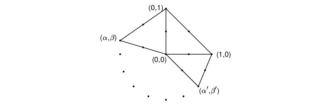
Figure 2: A local patch containing the reference triangle.

The next theorem gives practical criteria of checking the well-posedness of Rh0R_{h}^{0} and Rh1R_{h}^{1}.

Theorem 4.1

Let 𝐳\bm{z} be a vertex in 𝒯h\mathcal{T}_{h}. If #​𝒯​(ωz)≥5\#\mathcal{T}(\omega_{z})\geq 5 and the sum of each pair of adjacent angles in ωz\omega_{z} is ≤π\leq\pi, then there exists a unique 𝐪z\bm{q}_{z} at 𝐳\bm{z} for Rh0R_{h}^{0}. If #​𝒯​(ωz)≥4\#\mathcal{T}(\omega_{z})\geq 4, then there exists a unique 𝐪z\bm{q}_{z} at 𝐳\bm{z} for Rh1R_{h}^{1}.

Proof

Assume Πhr​𝒒z=0\Pi_{h}^{r}\bm{q}_{z}=0 on ωz\omega_{z}. By Lemma 4.2, 𝒒z=∇⟂w\bm{q}_{z}=\nabla^{\perp}w for some w∈𝒫r+2​(ωz)w\in\mathcal{P}_{r+2}(\omega_{z}). If r=0r=0, then w∈𝒫2​(ωz)w\in\mathcal{P}_{2}(\omega_{z}) vanishes at all vertices in ωz\omega_{z} and thus w=0w=0 by Theorem 2.3 in [22]. Hence 𝒒z=𝟎.\bm{q}_{z}=\bm{0}.

If r=1r=1, w∈𝒫3​(ωz)w\in\mathcal{P}_{3}(\omega_{z}) vanishes at all vertices and midpoints of edges in ωz\omega_{z}. Without loss of generality, we can assume that 𝒛=(0,0)\bm{z}=(0,0) and the reference triangle T^\hat{T} spanned by (0,0),(0,1),(1,0)(0,0),(0,1),(1,0) is in 𝒯h​(ωz)\mathcal{T}_{h}(\omega_{z}).

If ww is reducible, then the zero set w−1​(0)w^{-1}(0) is the union of three straight lines(counting multiplicity) or the union of a straight line and a conic. Clearly three lines cannot pass all vertices and midpoints in ωz\omega_{z} provided #​𝒯h​(ωz)≥4\#\mathcal{T}_{h}(\omega_{z})\geq 4. If w−1​(0)w^{-1}(0) contains a conic branch CC, then CC must contain at least two vertices 𝒂,𝒃\bm{a},\bm{b} in ωz\omega_{z} because #​𝒯h​(ωz)≥4\#\mathcal{T}_{h}(\omega_{z})\geq 4. However, CC cannot pass through (𝒂+𝒃)/2(\bm{a}+\bm{b})/2 by elementary geometry.

Hence reducible ww cannot vanish at all nodes in ωz\omega_{z} and we can assume

w=c1​x13+c2​x12​x2+c3​x1​x22+c4​x23+c5​x22+c6​x1​x2+c7​x22+c8​x1+c9​x2w=c_{1}x_{1}^{3}+c_{2}x_{1}^{2}x_{2}+c_{3}x_{1}x_{2}^{2}+c_{4}x_{2}^{3}+c_{5}x_{2}^{2}+c_{6}x_{1}x_{2}+c_{7}x_{2}^{2}+c_{8}x_{1}+c_{9}x_{2}

is irreducible. Furthermore, we can assume one of the coefficients of highest order terms is 11, say c1=1c_{1}=1(similar argument for c2,c3c_{2},c_{3} or c4=1c_{4}=1). Let (α,β)(\alpha,\beta) be the vertex outside T^\hat{T} next to (0,1)(0,1), see Fig. 2. Solving the linear system of equations

w⁡(1,0)=w⁡(0,1)=w⁡(1/2,0)=w⁡(0,1/2)=w⁡(1/2,1/2)\displaystyle w(1,0)=w(0,1)=w(1/2,0)=w(0,1/2)=w(1/2,1/2)
=w⁡(α,β)=w⁡(α2,β+12)=w⁡(α2,β2)=0,\displaystyle=w(\alpha,\beta)=w\left(\frac{\alpha}{2},\frac{\beta+1}{2}\right)=w\left(\frac{\alpha}{2},\frac{\beta}{2}\right)=0,

we have

c1=3−3​α1+β,c2=3​α​(α−1)β⁡(1+β).c_{1}=\frac{3-3\alpha}{1+\beta},\quad c_{2}=\frac{3\alpha(\alpha-1)}{\beta(1+\beta)}. (4.2)

Note that β≠0,β≠−1\beta\neq 0,\beta\neq-1 in (4.2), otherwise the irreducible cubic curve w−1​(0)w^{-1}(0) intersects with a line at five distinct points, which is impossible by Bézout’s theorem (see [25]). Also α≠1\alpha\neq 1 otherwise it violates the topology of the patch ωz\omega_{z}. Hence α/β=−c2/c1\alpha/\beta=-c_{2}/c_{1}. Let (α′,β′)(\alpha^{\prime},\beta^{\prime}) be the vertex outside T^\hat{T} next to (1,0)(1,0). Similarly we have α′/β′=−c2/c1\alpha^{\prime}/\beta^{\prime}=-c_{2}/c_{1}. Then it forces (α,β)=(α′,β′),(\alpha,\beta)=(\alpha^{\prime},\beta^{\prime}), which contradicts #​𝒯h​(ωz)≥4\#\mathcal{T}_{h}(\omega_{z})\geq 4. Hence w≡0w\equiv 0 and 𝒒z≡0.\bm{q}_{z}\equiv 0.

Therefore by Lemma 4.1, there exists a unique 𝒒z\bm{q}_{z} for r=0,1r=0,1. ∎

We say a vertex 𝒛\bm{z} is good if the condition in Theorem 4.1 holds at 𝒛\bm{z}, otherwise it is a bad vertex. In practice, 𝒯h\mathcal{T}_{h} typically has a few bad vertices, e.g., boundary vertices. There are several ways of dealing with a bad vertex 𝒛\bm{z}. If 𝒛\bm{z} is directly connected to a good vertex 𝒛′\bm{z}^{\prime}, one can define ωz:=ωz′\omega_{z}:=\omega_{z^{\prime}} and thus 𝑨z\bm{A}_{z} is of full column rank. A more convenient way is to empirically add some extra elements to the patch ωz\omega_{z} in practice, e.g., enlarge ωz\omega_{z} by one layer. Alternatively, one can solve a rank-deficient local least squares problem, which might reduce the rate of superconvergence of Rhr.R^{r}_{h}.

In the rest of this paper, we assume that

At each vertex 𝒛, there exists a unique 𝒒z.\text{At each vertex $\bm{z}$, there exists a unique $\bm{q}_{z}$}.

Using the uniqueness of the LS solution, we obtain the boundedness of RhrR_{h}^{r}.

Theorem 4.2

For 𝐪h∈𝒬hr\bm{q}_{h}\in\mathcal{Q}_{h}^{r} and T∈𝒯hT\in\mathcal{T}_{h},

∥Rhr𝒒∥0,T≲∥𝒒∥0,ωT,r=0,1.\|R_{h}^{r}\bm{q}\|_{0,T}\lesssim\|\bm{q}\|_{0,\omega_{T}},\quad r=0,1.
Proof

For 𝒛∈𝒩h,\bm{z}\in\mathcal{N}_{h}, Let σmin\sigma_{\min} and σmax\sigma_{\max} be the minimum and maximum singular values of 𝑨^z\hat{\bm{A}}_{z} respectively. The goal is to show that σmin\sigma_{\min} is uniformly bounded away from 00. MAC implies #​𝒯h​(ωz)≤Nmax=2​π/Θ\#\mathcal{T}_{h}(\omega_{z})\leq N_{\max}=2\pi/\Theta. Hence it suffices to consider the case #​𝒯h​(ωz)=N\#\mathcal{T}_{h}(\omega_{z})=N for some fixed N≤NmaxN\leq N_{\max}. In this case, #​ℰh​(ωz)=2​N\#\mathcal{E}_{h}(\omega_{z})=2N. Let N1=2​N,N2=6N_{1}=2N,N_{2}=6 provided r=0r=0 and N1=6​N,N2=12N_{1}=6N,N_{2}=12 provided r=1r=1. Let MN1×N2M_{N_{1}\times N_{2}} and SN1×N2S_{N_{1}\times N_{2}} be the set of N1×N2N_{1}\times N_{2} matrices and N1×N2N_{1}\times N_{2} rank-deficient matrices, respectively. It is well known that σmin=dist​(𝑨^z,SN1×N2)\sigma_{\min}=\text{dist}(\hat{\bm{A}}_{z},S_{N_{1}\times N_{2}}), the distance (measured by matrix 22-norm) from 𝑨^z\hat{\bm{A}}_{z} to rank-deficient matrices. dist​(⋅,SN1×N2)\text{dist}(\cdot,S_{N_{1}\times N_{2}}) is continuous on MN1×N2M_{N_{1}\times N_{2}}. Recall that 𝑨^z\hat{\bm{A}}_{z} is the scaled LS coefficient matrix determined by ωz\omega_{z}. Consider all possible ωz\omega_{z} and define

𝒜z={𝑨^z∈MN1×N2:#𝒯h(ωz)=N,ωz satisfies MAC}.\mathcal{A}_{z}=\{\hat{\bm{A}}_{z}\in M_{N_{1}\times N_{2}}:\#\mathcal{T}_{h}(\omega_{z})=N,\omega_{z}\text{ satisfies MAC}\}.

Clearly 𝒜z\mathcal{A}_{z} is a compact set in MN1×N2M_{N_{1}\times N_{2}} and any 𝑨^z∈𝒜z\hat{\bm{A}}_{z}\in\mathcal{A}_{z} is of full rank by the uniqueness assumption. Hence σmin=dist​(𝑨^z,SN1×N2)≥C1>0\sigma_{\min}=\text{dist}(\hat{\bm{A}}_{z},S_{N_{1}\times N_{2}})\geq C_{1}>0, where C1C_{1} depends only on the minimum angle Θ\Theta. The maximum singular value σmax≤C2\sigma_{\max}\leq C_{2}, where C2C_{2} only depends on Ω\Omega. For 𝒒h∈𝒬hr\bm{q}_{h}\in\mathcal{Q}_{h}^{r},

|𝒄^z|\displaystyle|\hat{\bm{c}}_{z}| ≤‖(𝑨^z⊺​𝑨^z)−1‖2​|𝑨^z⊺​𝒅z|≤σmin−2​σmax​|𝒅z|\displaystyle\leq\|(\hat{\bm{A}}_{z}^{\intercal}\hat{\bm{A}}_{z})^{-1}\|_{2}|\hat{\bm{A}}_{z}^{\intercal}\bm{d}_{z}|\leq\sigma_{\min}^{-2}\sigma_{\max}|\bm{d}_{z}| (4.3)
≤C1−2​C2​‖𝒒h‖0,∞,ωz≲hz−1​‖𝒒h‖0,ωz,\displaystyle\leq C_{1}^{-2}C_{2}\|\bm{q}_{h}\|_{0,\infty,\omega_{z}}\lesssim h_{z}^{-1}\|\bm{q}_{h}\|_{0,\omega_{z}},

where |⋅||\cdot| is the Euclidean norm. Finally by (4.3), we have

‖Rhr​𝒒h‖0,T≲h​‖Rhr​𝒒h‖0,∞,T≲h​|𝒄^z|≲‖𝒒h‖0,ωT,\|R_{h}^{r}\bm{q}_{h}\|_{0,T}\lesssim h\|R_{h}^{r}\bm{q}_{h}\|_{0,\infty,T}\lesssim h|\hat{\bm{c}}_{z}|\lesssim\|\bm{q}_{h}\|_{0,\omega_{T}},

which completes the proof. ∎

The super-approximation property of RhR_{h} follows from the uniqueness and boundedness results.

Theorem 4.3

For 𝐪∈Hr+2​(Ω)\bm{q}\in H^{r+2}(\Omega),

‖𝒒−Rhr​𝒒‖0,Ω≲hr+2|𝒒|r+2,Ω,r=0,1.\|\bm{q}-R_{h}^{r}\bm{q}\|_{0,\Omega}\lesssim h^{r+2}|\bm{q}|_{r+2,\Omega},\quad r=0,1.
Proof

Let T=𝒛1​𝒛2​𝒛3¯∈𝒯hT=\overline{\bm{z}_{1}\bm{z}_{2}\bm{z}_{3}}\in\mathcal{T}_{h} and T1⊂Ω¯T_{1}\subset\overline{\Omega} be a smallest local triangle containing ωT\omega_{T}. Let 𝒒r+1∈𝒫r+1​(T1)2\bm{q}_{r+1}\in\mathcal{P}_{r+1}(T_{1})^{2} be the degree-(r+1)(r+1) local Lagrange interpolant of 𝒒\bm{q} using based on T1T_{1}. By the uniqueness assumption, Rhr​𝒒r+1=𝒒r+1R_{h}^{r}\bm{q}_{r+1}=\bm{q}_{r+1} on TT. It then follows from Rhr​Πhr=RhrR_{h}^{r}\Pi_{h}^{r}=R_{h}^{r} that

‖𝒒−Rhr​𝒒‖0,T≤‖𝒒−𝒒r+1‖0,T+‖Rhr​Πhr​(𝒒r+1−𝒒)‖0,T.\|\bm{q}-R_{h}^{r}\bm{q}\|_{0,T}\leq\|\bm{q}-\bm{q}_{r+1}\|_{0,T}+\|R_{h}^{r}\Pi_{h}^{r}(\bm{q}_{r+1}-\bm{q})\|_{0,T}. (4.4)

Using the boundedness from Theorem 4.2, the stability in (2.3), and (1.6),

‖Rhr​Πhr​(𝒒r+1−𝒒)‖0,T≲‖Πhr​(𝒒r+1−𝒒)‖0,ωT\displaystyle\|R_{h}^{r}\Pi_{h}^{r}(\bm{q}_{r+1}-\bm{q})\|_{0,T}\lesssim\|\Pi_{h}^{r}(\bm{q}_{r+1}-\bm{q})\|_{0,\omega_{T}} (4.5)
≲h​‖Πhr​(𝒒r+1−𝒒)‖0,∞,ωT≲h​‖𝒒r+1−𝒒‖0,∞,ωT≲hr+2​|𝒒|r+2,T1.\displaystyle\lesssim h\|\Pi_{h}^{r}(\bm{q}_{r+1}-\bm{q})\|_{0,\infty,\omega_{T}}\lesssim h\|\bm{q}_{r+1}-\bm{q}\|_{0,\infty,\omega_{T}}\lesssim h^{r+2}|\bm{q}|_{r+2,T_{1}}.

Combining (4.4), (4.5) and the shape regularity 𝒯h\mathcal{T}_{h} completes the proof. ∎

In the end, we present the superconvergent recovery estimate.

Theorem 4.4

Assume that 𝒯h\mathcal{T}_{h} satisfies the (α,β)(\alpha,\beta)-condition. Then

∥𝒑−Rhr𝒑hr∥0,Ω≲hr+1+min⁡(12,α,β2)(|𝒑|r+1,∞,Ω+∥𝒑∥r+2,Ω),r=0,1.\|\bm{p}-R_{h}^{r}\bm{p}_{h}^{r}\|_{0,\Omega}\lesssim h^{r+1+\min(\frac{1}{2},\alpha,\frac{\beta}{2})}\big(|\bm{p}|_{r+1,\infty,\Omega}+\|\bm{p}\|_{r+2,\Omega}\big),\quad r=0,1.
Proof

The theorem follows from

‖𝒑−Rhr​𝒑hr‖0,Ω≤‖𝒑−Rhr​𝒑‖0,Ω+‖Rhr​(Πhr​𝒑−𝒑hr)‖0,Ω,\|\bm{p}-R_{h}^{r}\bm{p}_{h}^{r}\|_{0,\Omega}\leq\|\bm{p}-R_{h}^{r}\bm{p}\|_{0,\Omega}+\|R_{h}^{r}(\Pi_{h}^{r}\bm{p}-\bm{p}_{h}^{r})\|_{0,\Omega},

Theorems 4.2 and 4.3, Theorem 3.2(r=1r=1) or Theorem 4.5(r=0r=0) in [19]. ∎

5 Proof of Lemma 2.1

The following elementary triangular identities hold:

cosθk=(ℓk−12+ℓk+12−ℓk2)/(2ℓk−1ℓk+1),sinθk=ℓk/d,dk=ℓk−1ℓk+1/d,\displaystyle\cos\theta_{k}=(\ell_{k-1}^{2}+\ell_{k+1}^{2}-\ell_{k}^{2})/(2\ell_{k-1}\ell_{k+1}),\quad\sin\theta_{k}=\ell_{k}/d,\quad d_{k}=\ell_{k-1}\ell_{k+1}/d, (5.1)
𝒏k−1=−sinθk+1𝒕k−cosθk+1𝒏k,𝒏k+1=sinθk−1𝒕k−cosθk−1𝒏k,\displaystyle\bm{n}_{k-1}=-\sin\theta_{k+1}\bm{t}_{k}-\cos\theta_{k+1}\bm{n}_{k},\quad\bm{n}_{k+1}=\sin\theta_{k-1}\bm{t}_{k}-\cos\theta_{k-1}\bm{n}_{k},
∂𝒕k−12=cos2θk+1∂𝒕k2−2cosθk+1sinθk+1∂2𝒕k​𝒏k+sin2θk+1∂𝒏k2,\displaystyle\partial_{\bm{t}_{k-1}}^{2}{}=\cos^{2}\theta_{k+1}\partial_{\bm{t}_{k}}^{2}{}-2\cos\theta_{k+1}\sin\theta_{k+1}\partial^{2}_{\bm{t}_{k}\bm{n}_{k}}+\sin^{2}\theta_{k+1}\partial_{\bm{n}_{k}}^{2}{},
∂𝒕k+12=cos2θk−1∂𝒕k2+2cosθk−1sinθk−1∂2𝒕k​𝒏k+sin2θk−1∂𝒏k2.\displaystyle\partial_{\bm{t}_{k+1}}^{2}{}=\cos^{2}\theta_{k-1}\partial_{\bm{t}_{k}}^{2}{}+2\cos\theta_{k-1}\sin\theta_{k-1}\partial^{2}_{\bm{t}_{k}\bm{n}_{k}}+\sin^{2}\theta_{k-1}\partial_{\bm{n}_{k}}^{2}{}.

For each edge eke_{k}, we define several associated geometric quantities {αj​l,ki}1≤i,j,l≤2\{\alpha_{jl,k}^{i}\}_{1\leq i,j,l\leq 2}

α11,k1=124​d​ℓk2​ℓk−1​ℓk+1​(3​ℓk4−(ℓk−12−ℓk+12)2),\displaystyle\alpha^{1}_{11,k}=\frac{1}{24d\ell_{k}^{2}}\ell_{k-1}\ell_{k+1}\big(3\ell_{k}^{4}-(\ell_{k-1}^{2}-\ell_{k+1}^{2})^{2}\big),
α112,k=α121,k=112​d2​ℓkℓk−12ℓk+12(ℓk−12−ℓk+12),α122,k=−16​d3ℓk+13ℓk−13,\displaystyle\alpha^{1}_{12,k}=\alpha^{1}_{21,k}=\frac{1}{12d^{2}\ell_{k}}\ell_{k-1}^{2}\ell_{k+1}^{2}(\ell_{k-1}^{2}-\ell_{k+1}^{2}),\quad\alpha^{1}_{22,k}=-\frac{1}{6d^{3}}\ell_{k+1}^{3}\ell_{k-1}^{3},
α11,k2=148​ℓk3​(ℓk−12−ℓk+12)​(9​ℓk4−(ℓk−12−ℓk+12)2),\displaystyle\alpha^{2}_{11,k}=\frac{1}{48\ell_{k}^{3}}(\ell_{k-1}^{2}-\ell_{k+1}^{2})\big(9\ell_{k}^{4}-(\ell_{k-1}^{2}-\ell_{k+1}^{2})^{2}\big),
α212,k=α221,k=−α111,k,α222,k=−α112,k.\displaystyle\alpha^{2}_{12,k}=\alpha^{2}_{21,k}=-\alpha^{1}_{11,k},\quad\alpha^{2}_{22,k}=-\alpha^{1}_{12,k}.

To prove Lemma 2.1, we introduce cubic bubble functions

ψ0=λ1​λ2​λ3,ψk=λk−1​λk+1​(λk−1−λk+1),1≤k≤3.\psi_{0}=\lambda_{1}\lambda_{2}\lambda_{3},\quad\psi_{k}=\lambda_{k-1}\lambda_{k+1}(\lambda_{k-1}-\lambda_{k+1}),\quad 1\leq k\leq 3.

By counting the dimension, it is clear that {ψk}k=03\{\psi_{k}\}_{k=0}^{3} can span polynomials in 𝒫3​(T)\mathcal{P}_{3}(T) that vanish at {𝒛k}k=13\{\bm{z}_{k}\}_{k=1}^{3} and midpoints of {ek}k=13\{e_{k}\}_{k=1}^{3}. In fact, {ψk}k=03\{\psi_{k}\}_{k=0}^{3} has been used to derive superconvergence of quadratic Lagrange elements (cf.[15]) and a posteriori error estimators (cf.[5]).

Lemma 5.1

For 𝐩2∈𝒫2​(T)2\bm{p}_{2}\in\mathcal{P}_{2}(T)^{2},

𝒑2−Πh1​𝒑2=∇⟂w,\bm{p}_{2}-\Pi_{h}^{1}\bm{p}_{2}=\nabla^{\perp}w,

where

w=αj​l,βi​𝒟i,βj​l​(𝒑2)​ψ0+∑k=13ℓk312​𝒟2,k11​(𝒑2)​ψk,∀1≤β≤3.w=\alpha^{i}_{jl,\beta}\mathcal{D}_{i,\beta}^{jl}(\bm{p}_{2})\psi_{0}+\sum_{k=1}^{3}\frac{\ell_{k}^{3}}{12}\mathcal{D}_{2,k}^{11}(\bm{p}_{2})\psi_{k},\quad\forall 1\leq\beta\leq 3.
Proof

By Πh1​(𝒑2−Πh1​𝒑2)=0\Pi_{h}^{1}(\bm{p}_{2}-\Pi_{h}^{1}\bm{p}_{2})=0 and using Lemma 4.2, we have

𝒑2−Πh1​𝒑2=∇⟂(∑k=03ck​ψk).\bm{p}_{2}-\Pi_{h}^{1}\bm{p}_{2}=\nabla^{\perp}\big(\sum_{k=0}^{3}c_{k}\psi_{k}\big). (5.2)

For a unit vector 𝒅\bm{d} and the directional derivative ∂𝒅\partial_{\bm{d}}, the definition of ℛ​𝒯1​(T)\mathcal{RT}_{1}(T) implies that ∂𝒅2Πh1​𝒑2\partial_{\bm{d}}^{2}{\Pi_{h}^{1}\bm{p}_{2}} is proportional to 𝒅\bm{d}. Then applying 𝒅⟂⋅∂𝒅2\bm{d}^{\perp}\cdot\partial_{\bm{d}}^{2} to (5.2) gives

𝒅⟂⋅∂𝒅2𝒑2=∑k=03ck​∂𝒅3ψk.\bm{d}^{\perp}\cdot\partial_{\bm{d}}^{2}{\bm{p}_{2}}=\sum_{k=0}^{3}c_{k}\partial_{\bm{d}}^{3}\psi_{k}. (5.3)

By direct calculation,

∂𝒅3ψ0=6​∂𝒅λ1​∂𝒅λ2​∂𝒅λ3,\displaystyle\partial_{\bm{d}}^{3}\psi_{0}=6\partial_{\bm{d}}\lambda_{1}\partial_{\bm{d}}\lambda_{2}\partial_{\bm{d}}\lambda_{3}, (5.4a)
∂𝒅3ψk=6​∂𝒅λk−1​∂𝒅λk+1​(∂𝒅λk−1−∂𝒅λk+1),1≤k≤3.\displaystyle\partial_{\bm{d}}^{3}\psi_{k}=6\partial_{\bm{d}}\lambda_{k-1}\partial_{\bm{d}}\lambda_{k+1}(\partial_{\bm{d}}\lambda_{k-1}-\partial_{\bm{d}}\lambda_{k+1}),\quad 1\leq k\leq 3. (5.4b)

In particular, ∂𝒕k3ψ0=0\partial_{\bm{t}_{k}}^{3}\psi_{0}=0 and ∂𝒕k3ψj=−12δj​k/ℓk3.\partial_{\bm{t}_{k}}^{3}\psi_{j}=-12\delta_{jk}/\ell_{k}^{3}. By (5.4) and (5.3) with 𝒅=𝒕k\bm{d}=\bm{t}_{k}, we have

ck=ℓk312​𝒏k⋅∂𝒕k2𝒑2=ℓk312​𝒟2,k11​(𝒑2),1≤k≤3.c_{k}=\frac{\ell_{k}^{3}}{12}\bm{n}_{k}\cdot\partial_{\bm{t}_{k}}^{2}{\bm{p}_{2}}=\frac{\ell_{k}^{3}}{12}\mathcal{D}_{2,k}^{11}(\bm{p}_{2}),\quad 1\leq k\leq 3. (5.5)

It remains to determine c0c_{0}. (5.3) with 𝒅=𝒏k\bm{d}=\bm{n}_{k} implies that

𝒟1,k22​(𝒑2)=c0​∂𝒏k3ψ0+ck​∂𝒏k3ψk+ck−1​∂𝒏k3ψk−1+ck+1​∂𝒏k3ψk+1,\mathcal{D}_{1,k}^{22}(\bm{p}_{2})=c_{0}\partial_{\bm{n}_{k}}^{3}{\psi_{0}}+c_{k}\partial_{\bm{n}_{k}}^{3}{\psi_{k}}+c_{k-1}\partial_{\bm{n}_{k}}^{3}{\psi_{k-1}}+c_{k+1}\partial_{\bm{n}_{k}}^{3}{\psi_{k+1}}, (5.6)

By ∂𝒏kλk=−1/dk,∂𝒏kλk+1=cosθk−1/dk+1,∂𝒏kλk−1=cosθk+1/dk−1,\partial_{\bm{n}_{k}}\lambda_{k}=-1/d_{k},\partial_{\bm{n}_{k}}\lambda_{k+1}=\cos\theta_{k-1}/d_{k+1},\partial_{\bm{n}_{k}}\lambda_{k-1}=\cos\theta_{k+1}/d_{k-1}, (5.4) with 𝒅=𝒏k\bm{d}=\bm{n}_{k}, (5.5), and (5.6), we obtain

c0\displaystyle c_{0} =−dk−1​dk​dk+16cosθk−1cosθk+1​𝒟1,k22​(𝒑2)\displaystyle=-\frac{d_{k-1}d_{k}d_{k+1}}{6\cos\theta_{k-1}\cos\theta_{k+1}}\mathcal{D}_{1,k}^{22}(\bm{p}_{2}) (5.7)
+ℓk312​dk​(cos⁡θk+1dk−1−cos⁡θk−1dk+1)​𝒟2,k11​(𝒑2)\displaystyle+\frac{\ell_{k}^{3}}{12}d_{k}\left(\frac{\cos\theta_{k+1}}{d_{k-1}}-\frac{\cos\theta_{k-1}}{d_{k+1}}\right)\mathcal{D}_{2,k}^{11}(\bm{p}_{2})
−ℓk−1312​dk−1cos⁡θk+1​(1dk+cos⁡θk−1dk+1)​𝒟2,k−111​(𝒑2)\displaystyle-\frac{\ell_{k-1}^{3}}{12}\frac{d_{k-1}}{\cos\theta_{k+1}}\left(\frac{1}{d_{k}}+\frac{\cos\theta_{k-1}}{d_{k+1}}\right)\mathcal{D}_{2,k-1}^{11}(\bm{p}_{2})
+ℓk+1312​dk+1cos⁡θk−1​(1dk+cos⁡θk+1dk−1)​𝒟2,k+111​(𝒑2).\displaystyle+\frac{\ell_{k+1}^{3}}{12}\frac{d_{k+1}}{\cos\theta_{k-1}}\left(\frac{1}{d_{k}}+\frac{\cos\theta_{k+1}}{d_{k-1}}\right)\mathcal{D}_{2,k+1}^{11}(\bm{p}_{2}).

Then using (5.1) and (5.7), we obtain c0=αj​l,ki​𝒟i,kj​l​(𝒑2),1≤k≤3.c_{0}=\alpha^{i}_{jl,k}\mathcal{D}_{i,k}^{jl}(\bm{p}_{2}),1\leq k\leq 3. ∎

Now we can prove Lemma 2.1. In the proof, we shall use the integral formula

∫Tλ1m1​λ2m2​λ3m3=2​|T|​m1!​m2!​m3!(m1+m2+m3+2)!,∫eλ1m1​λ2m2=|e|​m1!​m2!(m1+m2+1)!,\int_{T}\lambda_{1}^{m_{1}}\lambda_{2}^{m_{2}}\lambda_{3}^{m_{3}}=\frac{2|T|m_{1}!m_{2}!m_{3}!}{(m_{1}+m_{2}+m_{3}+2)!},\quad\int_{e}\lambda_{1}^{m_{1}}\lambda_{2}^{m_{2}}=\frac{|e|m_{1}!m_{2}!}{(m_{1}+m_{2}+1)!}, (5.8)

where λ1,λ2\lambda_{1},\lambda_{2} are barycentric coordinates w.r.t. the edge ee.

Proof

Using (2.1) and Lemma 5.1, we have

∫T(𝒑2−Πh1​𝒑2)⋅∇⟂w2=∑k=13∫ekw​∇⟂w2⋅𝒕k−∫Tw​Δ​w2:=I+I​I.\displaystyle\int_{T}(\bm{p}_{2}-\Pi_{h}^{1}\bm{p}_{2})\cdot\nabla^{\perp}w_{2}=\sum_{k=1}^{3}\int_{e_{k}}w\nabla^{\perp}w_{2}\cdot\bm{t}_{k}-\int_{T}w\Delta w_{2}:=I+II. (5.9)

Recall that ϕk=λk−1​λk+1\phi_{k}=\lambda_{k-1}\lambda_{k+1} and let IhI_{h} be the linear interpolation. Then using the hierarchical representation

w2−Ihw2=−12∑k=13ℓk2ϕk∂𝒕k2w2,w_{2}-I_{h}w_{2}=-\frac{1}{2}\sum_{k=1}^{3}\ell_{k}^{2}\phi_{k}\partial_{\bm{t}_{k}}^{2}{w_{2}}, (5.10)

and Δϕk=2∇λk−1⋅∇λk+1=−2cosθk/(dk−1dk+1)\Delta\phi_{k}=2\nabla\lambda_{k-1}\cdot\nabla\lambda_{k+1}=-2\cos\theta_{k}/(d_{k-1}d_{k+1}), we obtain

Δw2=14​|T|2∑k=13ℓk2ℓk−1ℓk+1cosθk∂𝒕k2w2.\Delta w_{2}=\frac{1}{4|T|^{2}}\sum_{k=1}^{3}\ell_{k}^{2}\ell_{k-1}\ell_{k+1}\cos\theta_{k}\partial_{\bm{t}_{k}}^{2}w_{2}. (5.11)

It then follows from Lemma 5.1, (5.11), and ∫Tψ0=|T|/60,\int_{T}\psi_{0}=|T|/60, ∫Tψk=0,1≤k≤3,\int_{T}\psi_{k}=0,1\leq k\leq 3, that

II=−|T|60c0Δw2=−1240​|T|∑k=13c0ℓk2ℓk−1ℓk+1cosθk∂𝒕k2w2\displaystyle II=-\frac{|T|}{60}c_{0}\Delta w_{2}=-\frac{1}{240|T|}\sum_{k=1}^{3}c_{0}\ell_{k}^{2}\ell_{k-1}\ell_{k+1}\cos\theta_{k}\partial_{\bm{t}_{k}}^{2}{w_{2}} (5.12)
=−1120∑k=13∫ekαij​l,k𝒟i,kj​l(𝒑2)ℓkcotθk∂𝒕k2w2.\displaystyle=-\frac{1}{120}\sum_{k=1}^{3}\int_{e_{k}}\alpha^{i}_{jl,k}\mathcal{D}_{i,k}^{jl}(\bm{p}_{2})\ell_{k}\cot\theta_{k}\partial_{\bm{t}_{k}}^{2}{w_{2}}.

By the elementary identity 𝒕k=cos⁡θk+1sin⁡θk​𝒏k+1−cos⁡θk−1sin⁡θk​𝒏k−1,\bm{t}_{k}=\frac{\cos\theta_{k+1}}{\sin\theta_{k}}\bm{n}_{k+1}-\frac{\cos\theta_{k-1}}{\sin\theta_{k}}\bm{n}_{k-1}, Lemma 5.1, and ψk=−ℓk∂𝒕k(ϕk2)/2\psi_{k}=-\ell_{k}\partial_{\bm{t}_{k}}(\phi_{k}^{2})/2, we have

I\displaystyle I =−∑k=13112∫ekℓk3𝒟2,k11(𝒑2)ψk∇⟂w2⋅(cos⁡θk−1sin⁡θk𝒏k−1−cos⁡θk+1sin⁡θk𝒏k+1)\displaystyle=-\sum_{k=1}^{3}\frac{1}{12}\int_{e_{k}}\ell_{k}^{3}\mathcal{D}_{2,k}^{11}(\bm{p}_{2})\psi_{k}\nabla^{\perp}w_{2}\cdot\left(\frac{\cos\theta_{k-1}}{\sin\theta_{k}}\bm{n}_{k-1}-\frac{\cos\theta_{k+1}}{\sin\theta_{k}}\bm{n}_{k+1}\right) (5.13)
=∑k=13124​∫ekℓk4​𝒟2,k11​(𝒑2)​ϕk2​(cos⁡θk−1sin⁡θk​∂𝒕k​𝒕k−12w2−cos⁡θk+1sin⁡θk​∂𝒕k​𝒕k+12w2).\displaystyle=\sum_{k=1}^{3}\frac{1}{24}\int_{e_{k}}\ell_{k}^{4}\mathcal{D}_{2,k}^{11}(\bm{p}_{2})\phi^{2}_{k}\left(\frac{\cos\theta_{k-1}}{\sin\theta_{k}}\partial_{\bm{t}_{k}\bm{t}_{k-1}}^{2}w_{2}-\frac{\cos\theta_{k+1}}{\sin\theta_{k}}\partial_{\bm{t}_{k}\bm{t}_{k+1}}^{2}w_{2}\right).

Then using the quadrature rule (5.8),

I=1720​∑k=13ℓk5​𝒟2,k11​(𝒑2)​(cos⁡θk−1sin⁡θk​∂𝒕k​𝒕k−12w2−cos⁡θk+1sin⁡θk​∂𝒕k​𝒕k+12w2).\displaystyle I=\frac{1}{720}\sum_{k=1}^{3}\ell_{k}^{5}\mathcal{D}_{2,k}^{11}(\bm{p}_{2})\left(\frac{\cos\theta_{k-1}}{\sin\theta_{k}}\partial_{\bm{t}_{k}\bm{t}_{k-1}}^{2}w_{2}-\frac{\cos\theta_{k+1}}{\sin\theta_{k}}\partial_{\bm{t}_{k}\bm{t}_{k+1}}^{2}w_{2}\right).

In addition, (5.10) gives

∂𝒕k​𝒕k−12w2\displaystyle\partial_{\bm{t}_{k}\bm{t}_{k-1}}^{2}w_{2} =−ℓk2​ℓk−1∂𝒕k2w2+ℓk+122​ℓk−1​ℓk∂𝒕k+12w2−ℓk−12​ℓk∂𝒕k−12w2,\displaystyle=-\frac{\ell_{k}}{2\ell_{k-1}}\partial_{\bm{t}_{k}}^{2}{w_{2}}+\frac{\ell_{k+1}^{2}}{2\ell_{k-1}\ell_{k}}\partial_{\bm{t}_{k+1}}^{2}{w_{2}}-\frac{\ell_{k-1}}{2\ell_{k}}\partial_{\bm{t}_{k-1}}^{2}{w_{2}},
∂𝒕k​𝒕k+12w2\displaystyle\partial_{\bm{t}_{k}\bm{t}_{k+1}}^{2}w_{2} =−ℓk2​ℓk+1∂𝒕k2w2−ℓk+12​ℓk∂𝒕k+12w2+ℓk−122​ℓk​ℓk+1∂𝒕k−12w2.\displaystyle=-\frac{\ell_{k}}{2\ell_{k+1}}\partial_{\bm{t}_{k}}^{2}{w_{2}}-\frac{\ell_{k+1}}{2\ell_{k}}\partial_{\bm{t}_{k+1}}^{2}{w_{2}}+\frac{\ell_{k-1}^{2}}{2\ell_{k}\ell_{k+1}}\partial_{\bm{t}_{k-1}}^{2}{w_{2}}.

Therefore,

I\displaystyle I =11440∑k=13∫ek{ℓk5sin⁡θk𝒟2,k11(𝒑2)(cos⁡θk+1ℓk+1−cos⁡θk−1ℓk−1)\displaystyle=\frac{1}{1440}\sum_{k=1}^{3}\int_{e_{k}}\left\{\frac{\ell_{k}^{5}}{\sin\theta_{k}}\mathcal{D}_{2,k}^{11}(\bm{p}_{2})\left(\frac{\cos\theta_{k+1}}{\ell_{k+1}}-\frac{\cos\theta_{k-1}}{\ell_{k-1}}\right)\right. (5.14)
+ℓk−14sin⁡θk−1𝒟2,k−111(𝒑2)(cosθk+ℓkℓk+1cosθk+1)\displaystyle+\frac{\ell_{k-1}^{4}}{\sin\theta_{k-1}}\mathcal{D}_{2,k-1}^{11}(\bm{p}_{2})\left(\cos\theta_{k}+\frac{\ell_{k}}{\ell_{k+1}}\cos\theta_{k+1}\right)
−ℓk+14sin⁡θk+1𝒟2,k+111(𝒑2)(ℓkℓk−1cosθk−1+cosθk)}∂𝒕k2w2\displaystyle-\left.\frac{\ell_{k+1}^{4}}{\sin\theta_{k+1}}\mathcal{D}_{2,k+1}^{11}(\bm{p}_{2})\left(\frac{\ell_{k}}{\ell_{k-1}}\cos\theta_{k-1}+\cos\theta_{k}\right)\right\}\partial_{\bm{t}_{k}}^{2}w_{2}

Combining (5.9), (5.12), (5.14) and using (5.1), we obtain Lemma 2.1. ∎

6 Numerical experiments

Refer to caption
Figure 3: Delaunay initial grid on a square.
Refer to caption
Figure 4: (left)Regular refinement, 5504 elements. (right)Newest vertex bisection, 5504 elements.

We test our recovery operators RhrR_{h}^{r} with r=1,2,3r=1,2,3 by the Poisson equation

−Δ​u=f​ in ​Ω,-\Delta u=f\text{ in }\Omega,

where Ω\Omega and uu will be given in the next three experiments. Readers are referred to [19] for numerical results on recovery superconvergence of the R​T0RT_{0} element. The experiments are implemented using the iFEM package [8] in Matlab 2018b. In tables, ∥⋅∥\|\cdot\| is the L2L^{2}-norm ∥⋅∥0,Ω\|\cdot\|_{0,\Omega}, ‘nt’ denotes the number of triangles. The order of convergence is pp such that error≈\approx ndof−p2{}^{-\frac{p}{2}}, where ndof is the number of degrees of freedom. The value of pp is computed by least squares.

Problem 1. In the first experiment, let Ω\Omega be the unit square [0,1]2[0,1]^{2} and

u=exp⁡(x1+x2)​sin⁡(2​π​x1)​sin⁡(π​x2)u=\exp(x_{1}+x_{2})\sin(2\pi x_{1})\sin(\pi x_{2})

be the exact solution. We test the performance of Rh1R_{h}^{1}. Due to Theorem 4.1, we do not enlarge the patch ωz\omega_{z} when zz is an interior vertex. If zz is a boundary vertex, extra neighboring elements are added to ωz\omega_{z} such that #​ωz≥8.\#\omega_{z}\geq 8. It turns out that all local least squares problems are uniquely solvable. We start with the Delaunay triangulation in Fig. 3, and computed a sequence of meshes by regular refinement, i.e., dividing an element into four similar subelements by connecting the midpoints of each edge, see Table 1. We also computed a sequence of meshes by newest vertex bisection (cf. [20, 8]), see Fig. 4 and Table 2.

For regular refinement, the sequence of grids satisfies (α,β)(\alpha,\beta)-condition with (α,β)=(∞,1)(\alpha,\beta)=(\infty,1). For R​T1RT_{1} elements, Theorem 3.2 predicts that ‖Πh1​𝒑−𝒑h1‖=O⁡(h2.5)\|\Pi_{h}^{1}\bm{p}-\bm{p}_{h}^{1}\|=O(h^{2.5}), which is confirmed by Table 1. In view of the high order recovery superconvergence ‖𝒑−Rh1​𝒑h1‖=O⁡(h3.4)\|\bm{p}-R_{h}^{1}\bm{p}_{h}^{1}\|=O(h^{3.4}), our supercloseness estimate ‖𝒑−Rh1​𝒑h1‖=O⁡(h2.5)\|\bm{p}-R_{h}^{1}\bm{p}_{h}^{1}\|=O(h^{2.5}) in Theorem 4.4 may be suboptimal.

The sequence of grids created by newest vertex bisection is far from uniformly parallel, i.e., almost no pair of adjacent triangles forms an O⁡(h1+α)O(h^{1+\alpha}) approximate parallelogram with some positive α\alpha. Hence there is no supercloseness in Table 2. Surprisingly, we still observe apparent superconvergence for ‖𝒑−Rh1​𝒑h1‖\|\bm{p}-R_{h}^{1}\bm{p}_{h}^{1}\|.

Problem 2: Although our supercloseness estimates only work for R​T0RT_{0} and R​T1RT_{1} elements, we perform numerical experiments on the recovery operators Rh2R_{h}^{2} and Rh3R_{h}^{3} for R​T2RT_{2} and R​T3RT_{3} elements. We use the same Ω,u,\Omega,u, and initial mesh with regular refinement in Problem 1. Local patches ωz\omega_{z} is chosen in the same way as in Problem 1. The numerical results are presented in Tables 3 and 4.

As mentioned in Problem 1, the sequence of grids satisfies (α,β)(\alpha,\beta)-condition with (α,β)=(∞,1)(\alpha,\beta)=(\infty,1). Unlike R​T0RT_{0} and R​T1RT_{1} elements, there is no supercloseness phenomenon for R​T2RT_{2} and R​T3RT_{3} even on regularly refined meshes. However, it can be observed that the rate of recovery superconvergence is at least ‖𝒑−Rhr​𝒑hr‖=O⁡(hr+2)\|\bm{p}-R_{h}^{r}\bm{p}_{h}^{r}\|=O(h^{r+2}) with r=2,3r=2,3. Therefore, the supercloseness estimate is not a necessary ingredient of superconvergence analysis. We conjecture that the superconvergence is due to a large number of locally symmetric patches, see [24] for the theory of Lagrange elements.

Problem 3. Postprocessing superconvergence is often used to develop recovery-type a posteriori error estimator and adaptive FEMs. In the end, we test the adaptivity performance of Rh1R_{h}^{1} on the domain Ω=[−1,1]2\Ω0\Omega=[-1,1]^{2}\backslash\Omega_{0}, where Ω0\Omega_{0} is a right triangle whose smallest angle is ω=π/24\omega=\pi/24, see Fig. 5(left). Let

u⁡(r,θ)=rπ2​π−ω​sin⁡(π2​π−ω​θ)−r24,u(r,\theta)=r^{\frac{\pi}{2\pi-\omega}}\sin\left(\frac{\pi}{2\pi-\omega}\theta\right)-\frac{r^{2}}{4},

where (r,θ)(r,\theta) is the polar coordinate. The corresponding source f=−Δ​u=1f=-\Delta u=1. We use the classical adaptive feedback loop (cf. [10, 21])

SOLVE→ESTIMATE→MARK→REFINE.\textsf{SOLVE}\rightarrow\textsf{ESTIMATE}\rightarrow\textsf{MARK}\rightarrow\textsf{REFINE}.

It will return a sequence of meshes {𝒯hℓ}ℓ≥0\{\mathcal{T}_{h_{\ell}}\}_{\ell\geq 0} and numerical solutions {𝒑hℓ}ℓ≥0\{\bm{p}_{h_{\ell}}\}_{\ell\geq 0}. The algorithm starts from the initial grid 𝒯h0\mathcal{T}_{h_{0}} in Fig. 5(left). In the procedure ESTIMATE, ηℓ,T=‖Rhℓ1​𝒑hℓ1−𝒑hℓ1‖0,T\eta_{\ell,T}=\|R_{h_{\ell}}^{1}\bm{p}_{h_{\ell}}^{1}-\bm{p}_{h_{\ell}}^{1}\|_{0,T} serves as a posteriori error estimator on each triangle T∈𝒯hℓT\in\mathcal{T}_{h_{\ell}}. The procedure MARK selects a collection of triangles ℳℓ⊂𝒯hℓ\mathcal{M}_{\ell}\subset\mathcal{T}_{h_{\ell}} such that

∑T∈ℳℓηℓ,T2≥0.3​∑T∈𝒯hℓηℓ,T2.\sum_{T\in\mathcal{M}_{\ell}}\eta_{\ell,T}^{2}\geq 0.3\sum_{T\in\mathcal{T}_{h_{\ell}}}\eta_{\ell,T}^{2}.

Then the elements in ℳℓ\mathcal{M}_{\ell} and necessary neighboring elements are refined by local mesh refinement strategy to yield a conforming subtriangulation 𝒯hℓ+1\mathcal{T}_{h_{\ell+1}} of 𝒯hℓ\mathcal{T}_{h_{\ell}}. In particular, we use regular refinement with bisection closure in the procedure REFINE, see Fig. 5(right) for an adaptively refined triangulation. The numerical results are presented in Fig. 6.

It can be observed that the adaptive algorithm yields optimal rate of convergence and apparent recovery superconvergence. A distinct feature of the a posteriori error estimator ηhℓ:=‖Rhℓ1​𝒑hℓ1−𝒑hℓ1‖0,Ω=(∑T∈𝒯hℓηℓ,T2)12\eta_{h_{\ell}}:=\|R_{h_{\ell}}^{1}\bm{p}_{h_{\ell}}^{1}-\bm{p}_{h_{\ell}}^{1}\|_{0,\Omega}=\big(\sum_{T\in\mathcal{T}_{h_{\ell}}}\eta_{\ell,T}^{2}\big)^{\frac{1}{2}} is the well-known asymptotic exactness:

limℓ→∞ηhℓ‖𝒑−𝒑hℓ1‖0,Ω=1,\displaystyle\lim_{\ell\rightarrow\infty}\frac{\eta_{h_{\ell}}}{\|\bm{p}-\bm{p}^{1}_{h_{\ell}}\|_{0,\Omega}}=1,

which can be numerically confirmed using the rates of superconvergence in Fig. 6 with a triangle inequality, see, e.g., [4, 27] for details.

Table 1: R​T1RT_{1} with regular refinement
nt ‖𝒑−𝒑h1‖\|\bm{p}-\bm{p}_{h}^{1}\| ‖Πh1​𝒑−𝒑h1‖\|\Pi_{h}^{1}\bm{p}-\bm{p}_{h}^{1}\| ‖𝒑−Rh1​𝒑h1‖\|\bm{p}-R_{h}^{1}\bm{p}_{h}^{1}\|
86 3.176e-1 4.297e-2 5.186e-1
344 8.000e-2 7.852e-3 5.560e-2
1376 2.006e-2 1.397e-3 5.344e-3
5504 5.022e-3 2.461e-4 4.929e-4
22106 1.256e-3 4.336e-5 4.616e-5
order 1.998 2.501 3.414
Table 2: R​T1RT_{1} with bisection refinement
nt ‖𝒑−𝒑h1‖\|\bm{p}-\bm{p}_{h}^{1}\| ‖Πh1​𝒑−𝒑h1‖\|\Pi_{h}^{1}\bm{p}-\bm{p}_{h}^{1}\| ‖𝒑−Rh1​𝒑h1‖\|\bm{p}-R_{h}^{1}\bm{p}_{h}^{1}\|
86 3.176e-1 4.297e-2 5.186e-1
344 1.325e-1 1.092e-1 7.453e-2
1376 3.401e-2 2.682e-2 1.005e-2
5504 8.604e-3 6.607e-3 1.610e-3
22016 2.164e-3 1.637e-3 3.336e-4
order 1.979 2.020 2.605
Table 3: R​T2RT_{2} with regular refinement
nt ‖𝒑−𝒑h2‖\|\bm{p}-\bm{p}_{h}^{2}\| ‖Πh2​𝒑−𝒑h2‖\|\Pi_{h}^{2}\bm{p}-\bm{p}_{h}^{2}\| ‖𝒑−Rh2​𝒑h2‖\|\bm{p}-R_{h}^{2}\bm{p}_{h}^{2}\|
86 2.378e-2 5.201e-3 1.505e-1
344 3.022e-3 5.488e-4 1.005e-2
1376 3.792e-4 6.501e-5 5.247e-4
5504 4.745e-5 8.002e-6 2.551e-5
22106 5.933e-6 9.953e-7 1.351e-6
order 2.993 3.080 4.215
Table 4: R​T3RT_{3} with regular refinement
nt ‖𝒑−𝒑h3‖\|\bm{p}-\bm{p}_{h}^{3}\| ‖Πh3​𝒑−𝒑h3‖\|\Pi_{h}^{3}\bm{p}-\bm{p}_{h}^{3}\| ‖𝒑−Rh3​𝒑h3‖\|\bm{p}-R_{h}^{3}\bm{p}_{h}^{3}\|
86 3.733e-3 3.394e-3 4.022e-2
344 2.359e-4 2.140e-4 1.180e-3
1376 1.478e-5 1.338e-5 2.668e-5
5504 9.242e-7 8.354e-7 6.377e-7
22106 5.777e-8 5.217e-8 2.116e-8
order 3.995 3.998 5.257
Refer to caption
Figure 5: (left)Initial grid for the adaptive algorithm. (right)Adaptive grid, 2026 elements.
Refer to caption
Figure 6: Error curves for R​T1RT_{1}.

7 Concluding remarks

In this paper, we develop supercloseness estimate for the second lowest order RT element and a family of postprocessing operators RhrR_{h}^{r} for higher order RT elements applied to second order elliptic equations. Since both the analysis of supercloseness and postprocessing operators are local, our superconvergence results can be adapted to Neumann and mixed boundary conditions. In practice, RhrR_{h}^{r} can be extended to 3-dimensional RT elements in a straightforward way although the theoretical analysis in this paper may need significant modifications, e.g., the supercloseness estimate and well-posedness of the local least squares problem would be more complicated. Readers are also referred to [13] for numerical experiments on a different postprocessing operator for the lowest order RT elements in ℝ3\mathbb{R}^{3}.

References

  • (1) Arnold, D.N., Falk, R.S., Winther, R.: Finite element exterior calculus, homological techniques, and applications. Acta Numer. 15, 1–155 (2006)
  • (2) Arnold, D.N., Falk, R.S., Winther, R.: Finite element exterior calculus: from Hodge theory to numerical stability. Bull. Amer. Math. Soc. 47(2), 281–354 (2010)
  • (3) Bank, R.E., Xu, J.: Asymptotically exact a posteriori error estimators. I. grids with superconvergence. SIAM J. Numer. Anal. 41(6), 2294–2312 (2003)
  • (4) Bank, R.E., Xu, J.: Asymptotically exact a posteriori error estimators. II. general unstructured grids. SIAM J. Numer. Anal. 41(6), 2313–2332 (2003)
  • (5) Bank, R.E., Xu, J., Zheng, B.: Superconvergent derivative recovery for lagrange triangular elements of degree p on unstructured grids. SIAM J. Numer. Anal. 45(5), 2032–2046 (2007)
  • (6) Brandts, J.H.: Superconvergence and a posteriori error estimation for triangular mixed finite elements. Numer. Math. 68(3), 311–324 (1994)
  • (7) Brandts, J.H.: Superconvergence for triangular order k=1 raviart-thomas mixed finite elements and for triangular standard quadratic finite element methods. Appl. Numer. Math. 34(1), 39–58 (2000)
  • (8) Chen, L.: iFEM: an innovative finite element method package in Matlab (2009). University of California Irvine, Technical report
  • (9) Chen, L., Holst, M., Xu, J.: Convergence and optimality of adaptive mixed finite element methods. Math. Comp. 78(265), 35–53 (2009)
  • (10) Dörfler, W.: A convergent adaptive algorithm for Poisson’s equation. SIAM J. Numer. Anal. 33(3), 1106–1124 (1996)
  • (11) Douglas J., J., Milner, F.A.: Interior and superconvergence estimates for mixed methods for second order elliptic problems. RAIRO Modél. Math. Anal. Numér. 19(3), 397–428 (1985)
  • (12) Douglas Jim, J., Roberts, J.E.: Global estimates for mixed methods for second order elliptic equations. Math. Comp. 44(169), 39–52 (1985)
  • (13) Dupont, T.F., Keenan, P.T.: Superconvergence and postprocessing of fluxes from lowest-order mixed methods on triangles and tetrahedra. SIAM J. Sci. Comput. 19(4), 1322–1332 (1998)
  • (14) Durán, R.: Superconvergence for rectangular mixed finite elements. Numer. Math. 58(3), 287–298 (1990)
  • (15) Huang, Y., Xu, J.: Superconvergence of quadratic finite elements on mildly structured grids. Math. Comp. 77(263), 1253–1268 (2008)
  • (16) Lakhany, A.M., Marek, I., Whiteman, J.R.: Superconvergence results on mildly structured triangulations. Comput. Methods Appl. Mech. Engrg. 189, 1–75 (2000)
  • (17) Li, B., Zhang, Z.: Analysis of a class of superconvergence patch recovery techniques for linear and bilinear finite elements. Numer. Methods Partial Differential Equations 15(2), 151–167 (1999)
  • (18) Li, Y.: Some convergence and optimality results of adaptive mixed methods in finite element exterior calculus. SIAM J. Numer. Anal. 57(4), 2019–2042 (2019)
  • (19) Li, Y.W.: Global superconvergence of the lowest-order mixed finite element on mildly structured meshes. SIAM J. Numer. Anal. 56(2), 792–815 (2018)
  • (20) Mitchell, W.F.: A comparison of adaptive refinement techniques for elliptic problems. ACM Trans. Math. Software 15(4), 326–347 (1989)
  • (21) Morin, P., Nochetto, R.H., Siebert, K.G.: Data oscillation and convergence of adaptive FEM. SIAM J. Numer. Anal. 38(2), 466–488 (2000)
  • (22) Naga, A., Zhang, Z.: A posteriori error estimates based on the polynomial preserving recovery. SIAM J. Numer. Anal. 42(4), 1780–1800 (2004)
  • (23) Raviart, P.A., Thomas, J.M.: A mixed finite element method for 2nd order elliptic problems, Lecture Notes in Mathematics, vol. 606, pp. 292–315. Springer, Berlin (1977)
  • (24) Schatz, A.H., Sloan, I.H., Wahlbin, L.B.: Superconvergence in finite element methods and meshes that are locally symmetric with respect to a point. SIAM J. Numer. Anal. 33(2), 505–521 (1996)
  • (25) Shafarevich, I.R.: Basic algebraic geometry. 1. Varieties in projective space, thrid edition edn. Springer, Heidelberg (2013)
  • (26) Wu, H., Zhang, Z.: Can we have superconvergent gradient recovery under adaptive meshes? SIAM J. Numer. Anal. 45(4), 1701–1722 (2007)
  • (27) Xu, J., Zhang, Z.: Analysis of recovery type a posteriori error estimators for mildly structured grids. Math. Comp. 73(247), 1139–1152 (2004)
  • (28) Zhang, Z., Naga, A.: A new finite element gradient recovery method: superconvergence property. SIAM J. Sci. Comput. 26(4), 1192–1213 (2005)
  • (29) Zienkiewicz, O.C., Zhu, J.: The superconvergent patch recovery and a posteriori error estimates. II. error estimates and adaptivity. Internat. J. Numer. Methods Engrg. 33(7), 1365–1382 (1992)
  • (30) Zienkiewicz, O.C., Zhu, J.Z.: The superconvergent patch recovery and a posteriori error estimates. I. the recovery technique. Internat. J. Numer. Methods Engrg. 33(7), 1331–1364 (1992)