Large-Scale Sparse Inverse Covariance Estimation via Thresholding and Max-Det Matrix CompletionThanks: Proceedings of the 35-th International Conference on Machine Learning, Stockholm, Sweden, PMLR 80, 2018. Copyright 2018 by the author(s). This work was supported by the ONR grants N00014-17-1-2933 and N00014-15-1-2835, DARPA grant D16AP00002, and AFOSR grant FA9550-17-1-0163.

The high practical cost of graphical lasso has inspired a number of heuristics, which enjoy less guarantees but are significantly cheaper to use. Indeed, heuristics are often the only viable option once $n$ exceeds the order of a few tens of thousands.

One simple idea is to threshold the sample covariance matrix $C$: to examine all of its elements and keep only the ones whose magnitudes exceed some threshold. Thresholding can be fast—even for very large-scale datasets—because it is embarassingly parallel; its quadratic $O(n^{2})$ total work can be spread over thousands or millions of parallel processors, in a GPU or distributed on cloud servers. When the number of samples $N$ is small, i.e. $N\ll n$, thresholding can also be performed using $O(n)$ memory, by working directly with the $n\times N$ centered matrix-of-samples $\mathbf{X}=[\mathbf{x}_{1}-\bar{\mathbf{x}},\mathbf{x}_{2}-\bar{\mathbf{x}},\ldots,\mathbf{x}_{N}-\bar{\mathbf{x}}]$ satisfying $C=\frac{1}{N}\mathbf{X}\mathbf{X}^{T}$.

In a recent line of work [26, 39, 12, 13], the simple heuristic of thresholding was shown to enjoy some surprising guarantees. In particular, [39, 12] proved that when the lasso weight is imposed over only the off-diagonal elements of $X$ that—under some assumptions—the sparsity pattern of the associated graphical lasso estimator can be recovered by performing a soft-thresholding operation on $C$, as in

$$(C_{\lambda})_{i,j}=\begin{cases}C_{i,j}&i=j,\\ C_{i,j}-\lambda&C_{i,j}>\lambda,\;i\not=j,\\ 0&|C_{i,j}|\leq\lambda\;i\not=j,\\ C_{i,j}+\lambda&-\lambda\leq C_{i,j}\,i\not=j,\end{cases}$$

(2)

and recovering

$$G=\{(i,j)\in\{1,\ldots,n\}^{2}:(C_{\lambda})_{i,j}\neq 0\}.$$

(3)

The associated graph (also denoted as $G$ when there is no ambiguity) is obtained by viewing each nonzero element $(i,j)$ in $G$ as an edge between the $i$-th and $j$-th vertex in an undirected graph on $n$ nodes. Moreover, they showed that the estimator $X$ can be recovered by solving a version of (1) in which the sparsity pattern $G$ is explicitly imposed, as in

	$\displaystyle\underset{X\succ 0}{\text{minimize }}$	$\displaystyle\mathrm{tr}\,C_{\lambda}X-\log\det X$		(4)
	subject to	$\displaystyle X_{i,j}=0\quad\forall(i,j)\notin G.$

Recovering the exact value of $X$ (and not just its sparsity pattern) is important because it provides a shrinkage MLE when the true MLE is ill-defined; for Gaussian fields, its nonzero values encode the partial correlations between variables. Problem (4) is named the maximum determinant matrix completion (MDMC) in the literature, for reasons explained below. The problem has a recursive closed-form solution whenever the graph of $G$ is acyclic (i.e. a tree or forest) [12], or more generally, if it is chordal [13]. It is worth emphasizing that the closed-form solution is extremely fast to evaluate: a chordal example in [13] with 13,659 variables took just $\approx 5$ seconds to solve on a laptop computer.

The assumptions needed for graphical lasso to be equivalent to thresolding are hard to check but relatively mild. Indeed, [12] proves that they are automatically satisfied whenever $\lambda$ is sufficiently large relative to the sample covariance matrix. Their numerical study found “sufficiently large” to be a fairly loose criterion in practice, particularly in view of the fact that large values of $\lambda$ are needed to induce a sufficiently sparse estimate of $\Sigma^{-1}$, e.g. with $\approx 10n$ nonzero elements.

However, the requirement for $G$ to be chordal is very strong. Aside from trivial chordal graphs like trees and cliques, thresholding will produce a chordal graph with probability zero. When $G$ is nonchordal, no closed-form solution exists, and one must resort to an iterative algorithm. The state-of-the-art for nonchordal MDMC is to embed the nonchordal graph within a chordal graph, and to solve the resulting problem as a semidefinite program using an interior-point method [8, 2].

The purpose of this paper is two-fold. First, we derive an extension of the guarantees derived by [26, 39, 12, 13] for a slightly more general version of the problem that we call restricted graphical lasso (RGL):

	$\displaystyle\hat{X}=\underset{X\succ 0}{\text{minimize }}$	$\displaystyle\mathrm{tr}\,CX-\log\det X+\sum_{i=1}^{n}\sum_{j=i+1}^{n}\lambda_{i,j}|X_{i,j}|$		(5)
	subject to	$\displaystyle X_{i,j}=0\qquad\forall(i,j)\notin H.$

In other words, RGL is (1) penalized by a weighted lasso penalty $\lambda_{i,j}$ on the off-diagonals, and with an a priori sparsity pattern $H$ imposed as an additional constraint. We use the sparsity pattern $H$ to incorporate prior information on the structure of the graphical model. For example, if the sample covariance $C$ is collected over a graph, such as a communication system or a social network, then far-away variables can be assumed as pairwise conditionally independent [33, 19, 7]. Including these neighborhood relationships into $H$ can regularize the statistical problem, as well as reduce the numerical cost for a solution.

In Section 2, we describe a procedure to transform RGL (5) into MDMC (4), in the same style as prior results by [12, 13] for graphical lasso. More specifically, we soft-threshold the sample covariance $C$ and then project this matrix onto the sparsity pattern $H$. We give conditions for the resulting sparsity pattern to be equivalent to the one obtained by solving (5). Furthermore, we prove that the resulting estimator $X$ can be recovered by solving the same MDMC problem (4) with $C_{\lambda}$ appropriately modified.

The second purpose is to describe an efficient algorithm to solve MCDC when the graph $G$ is nonchordal, based on the chordal embedding approach of [8, 2, 4]. We embed $G$ within a chordal $\tilde{G}\supset G$, to result in a convex optimization problem over $\mathbb{S}_{\tilde{G}}^{n}$, the space of real symmetric matrices with sparsity pattern $\tilde{G}$. This way, the constraint $X\in\mathbb{S}_{\tilde{G}}^{n}$ is implicitly imposed, meaning that we simply ignore the nonzero elements not in $\tilde{G}$. Next, we solve an optimization problem on $\mathbb{S}_{\tilde{G}}^{n}$ using a custom Newton-CG method¹¹ 1 The MATLAB source code for our solver can be found at http://alum.mit.edu/www/ryz. The main idea is to use an inner conjugate gradients (CG) loop to solve the Newton subproblem of an outer Newton’s method. The actual algorithm has a number of features designed to exploit problem structure, including the sparse chordal property of $\tilde{G}$, duality, and the ability for CG and Newton to converge superlinearly; these are outlined in Section 3.

Assuming that the chordal embedding is sparse with $|\tilde{G}|=O(n)$ nonzero elements, we prove in Section 3.4, that our algorithm converges to an $\epsilon$-accurate solution of MDMC (4) in

$$O(n\cdot\log\epsilon^{-1}\cdot\log\log\epsilon^{-1})\text{ time and }O(n)\text{ memory.}$$

(6)

Most importantly, the algorithm is highly efficient in practice. In Section 4, we present computation results on a suite of test cases. Both synthetic and real-life graphs are considered. Using our approach, we solve sparse inverse covariance estimation problems containing as many as 200,000 variables, in less than an hour on a laptop computer.

Graphical lasso with prior information. A number of approaches are available in the literature to introduce prior information to graphical lasso. The weighted version of graphical lasso mentioned before is an example, though RGL will generally be more efficient to solve due to a reduction in the number of variables. [11] introduced a class of graphical lasso in which the true graphical model is assumed to have Laplacian structure. This structure commonly appears in signal and image processing [28]. For the a priori graph-based correlation structure described above, [17] introduced a pathway graphical lasso method similar to RGL.

Algorithms for graphical lasso. Algorithms for graphical lasso are usually based on some mixture of Newton [32], proximal Newton [21, 20], iterative thresholding [35], and (block) coordinate descent [14, 40]. All of these suffer fundamentally from the need to keep track and act on all $O(n^{2})$ elements in the matrix $X$ decision variable. Even if the final solution matrix were sparse with $O(n)$ nonzeros, it is still possible for the algorithm to traverse through a “dense region” in which the iterate $X$ must be fully dense. Thresholding heuristics have been proposed to address issue, but these may adversely affect the outer algorithm and prevent convergence. It is generally impossible to guarantee a figure lower than $O(n^{2})$ time per-iteration, even if the solution contains only $O(n)$ nonzeros. Most of the algorithms mentioned above actually have worst-case per-iteration costs of $O(n^{3})$.

Graphical lasso via thresholding. The elementary estimator for graphical models (EE-GM) [43] is another thresholding-based low-complexity method that is able to recover the actual graphical lasso estimator. Both EE-GM and our algorithm have a similar level of performance in practice, because both algorithm are bottlenecked by the initial thresholding step, which is a quadratic $O(n^{2})$ time operation.

Algorithms for MDMC. Our algorithm is inspired by a line of results [8, 2, 4, 23] for minimizing the log-det penalty on chordal sparsity patterns, culminating in the CVXOPT package [3]. These are Newton algorithms that solve the Newton subproblem by explicitly forming and factoring the fully-dense Newton matrix. When $|\tilde{G}|=O(n)$, these algorithms cost $O(nm^{2}+m^{3})$ time and $O(m^{2})$ memory per iteration, where $m$ is the number of edges added to $G$ to yield the chordal $\tilde{G}$. In practice, $m$ is usually a factor of 0.1 to 20 times $n$, so these algorithms are cubic $O(n^{3})$ time and $O(n^{2})$ memory. Our algorithm solves the Newton subproblem iteratively using CG. We prove that CG requires just $O(n)$ time to compute the Newton direction to machine precision (see Section 3.4). In practice, CG converges much faster than its worst-case bound, because it is able to exploit eigenvalue clustering to achieve superlinear convergence.

Let $\mathbb{R}^{n}$ be the set of $n\times 1$ real vectors, and $\mathbb{S}^{n}$ be the set of $n\times n$ real symmetric matrices. (We denote $x\in\mathbb{R}^{n}$ using lower-case, $X\in\mathbb{S}^{n}$ using upper-case, and index the $(i,j)$-th element of $X$ as $X_{i,j}$.) We endow $\mathbb{S}^{n}$ with the usual matrix inner product $X\bullet Y=\mathrm{tr}\,XY$ and Euclidean (i.e. Frobenius) norm $\|X\|_{F}^{2}=X\bullet X$. Let $\mathbb{S}_{+}^{n}\subset\mathbb{S}^{n}$ and $\mathbb{S}_{++}^{n}\subset\mathbb{S}_{+}^{n}$ be the associated set of positive semidefinite and positive definite matrices. We will frequently write $X\succeq 0$ to mean $X\in\mathbb{S}_{+}^{n}$ and write $X\succ 0$ to mean $X\in\mathbb{S}_{++}^{n}$. Given a sparsity pattern $G$, we define $\mathbb{S}_{G}^{n}\subseteq\mathbb{S}^{n}$ as the set of $n\times n$ real symmetric matrices with this sparsity pattern.

Following [8], we begin by reformulating (4) into a sparse chordal matrix program

	$\displaystyle\hat{X}=\text{ minimize }$	$\displaystyle\mathrm{tr}\,CX-\log\det X$		(12)
	subject to	$\displaystyle X_{i,j}=0\quad\forall(i,j)\in\tilde{G}\backslash G.$
		$\displaystyle X\in\mathbb{S}_{\tilde{G}}^{n}.$

in which $\tilde{G}$ is a chordal embedding for $G$: a sparsity pattern $\tilde{G}\supset G$ whose graph contains no induced cycles greater than three. This can be implemented using standard algorithms for large-and-sparse linear equations, due to the following result.

Note that $\tilde{G}$ can be determined directly from $G$ using a symbolic Cholesky algorithm, which simulates the steps of Gaussian elimination using Boolean logic. Moreover, we can substantially reduce the number of edges added to $G$ by reordering the columns and rows of $C$ using a fill-reducing ordering.

The problem of finding the best choice of $\Pi$ is known as the fill-minimizing problem, and is NP-complete [44]. However, good orderings are easily found using heuristics developed for numerical linear algebra, like minimum degree ordering [15] and nested dissection [16, 1]. In fact, [16] proved that nested dissection is $O(\log(n))$ suboptimal for bounded-degree graphs, and notes that “we do not know a class of graphs for which [nested dissection is suboptimal] by more than a constant factor.”

If $G$ admits sparse chordal embeddings, then a good-enough $|\tilde{G}|=O(n)$ will usually be found using minimum degree or nested dissection. In MATLAB, the minimum degree ordering and symbolic factorization steps can be performed in two lines of code; see the snippet in Figure 1.

Define the cone of sparse positive semidefinite matrices $\mathcal{K}$, and the cone of sparse matrices with positive semidefinite completions $\mathcal{K}_{*}$, as the following

$$\mathcal{K}=\mathbb{S}_{+}^{n}\cap\mathbb{S}_{\tilde{G}}^{n},\qquad\mathcal{K}_{*}=\{S\bullet X\geq 0:S\in\mathbb{S}_{\tilde{G}}\}=P_{\tilde{G}}(\mathbb{S}_{+}^{n}).$$

Then (12) can be posed as the primal-dual pair:

	$\displaystyle\arg\min_{X\in\mathcal{K}}$	$\displaystyle\{C\bullet X+f(X):A^{T}(X)=0\},$		(13)
	$\displaystyle\arg\max_{S\in\mathcal{K}_{*},y\in\mathbb{R}^{m}}$	$\displaystyle\{-f_{*}(S):S=C-A(y)\},$		(14)

with in which $f$ and $f_{*}$ are the “log-det” barrier functions on $\mathcal{K}$ and $\mathcal{K}_{*}$ as introduced by [8, 2, 4]

$$f(X)=-\log\det X,\qquad f_{*}(S)=-\min_{X\in\mathcal{K}}\{S\bullet X-\log\det X\}.$$

The linear map $A:\mathbb{R}^{m}\to\mathbb{S}_{\tilde{G}\backslash G}^{n}$ converts a list of $m$ variables into the corresponding matrix in $\tilde{G}\backslash G$. The gradients of $f$ are simply the projections of their usual values onto $\mathbb{S}_{\tilde{G}}^{n}$, as in

$$\nabla f(X)=-P_{\tilde{G}}(X^{-1}),\qquad\nabla^{2}f(X)[Y]=P_{\tilde{G}}(X^{-1}YX^{-1}).$$

Given any $S\in\mathcal{K}_{*}$ let $X\in\mathcal{K}$ be the unique matrix satisfying $P_{\tilde{G}}(X^{-1})=S$. Then we have

$$f_{*}(S)=n+\log\det X,\qquad\nabla f_{*}(S)=-X,\qquad\nabla^{2}f_{*}(S)[Y]=\nabla^{2}f(X)^{-1}[Y].$$

Assuming that $\tilde{G}$ is sparse and chordal, all six operations can be efficiently evaluated in $O(n)$ time and $O(n)$ memory, using the numerical recipes described in [4].

Our algorithm actually solves the dual problem (14), which can be rewritten as an unconstrained optimization problem

$$\hat{y}\equiv\arg\min_{y\in\mathbb{R}^{m}}g(y)\equiv f_{*}(C_{\lambda}-A(y)).$$

(15)

After the solution $\hat{y}$ is found, we can recover the optimal estimator for the primal problem via $\hat{X}=-\nabla f_{*}(C_{\lambda}-A(y))$. The dual problem (14) is easier to solve than the primal (13) because the origin $y=0$ often lies very close to the solution $\hat{y}$. To see this, note that $y=0$ produces a candidate estimator $\tilde{X}=-\nabla f_{*}(C_{\lambda})$ that solves the chordal matrix completion problem

$$\tilde{X}=\arg\min\{\mathrm{tr}\,C_{\lambda}X-\log\det X:X\in\mathbb{S}_{\tilde{G}}^{n}\},$$

which is a relaxation of the nonchordal problem posed over $\mathbb{S}_{G}^{n}$. As observed by several previous authors [8], this relaxation is a high quality guess, and $\tilde{X}$ is often “almost feasible” for the original nonchordal problem posed over $\mathbb{S}_{G}^{n}$, as in $\tilde{X}\approx P_{G}(\tilde{X})$. Some simple algebra shows that the gradient $\nabla g$ evaluated at the origin has Euclidean norm $\|\nabla g(0)\|=\|\tilde{X}-P_{G}(\tilde{X})\|_{F}$, so if $\tilde{X}\approx P_{G}(\tilde{X})$ holds true, then the origin $y=0$ is close to optimal. Starting from this point, we can expect Newton’s method to rapidly converge at a quadratic rate.

The most computationally expensive part of Newton’s method is the solution of the Newton direction $\Delta y$ via the $m\times m$ system of equations

$$\nabla^{2}g(y)\Delta y=-\nabla g(y).$$

(16)

The Hessian matrix $\nabla^{2}g(y)$ is fully dense, but matrix-vector products are linear $O(n)$ time using the algorithms in Section . This insight motivates solving (16) using an iterative Krylov subspace method like conjugate gradients (CG), which is a matrix-free method that requires a single matrix-vector product with $\nabla^{2}g(y)$ at each iteration [6]. Starting from the origin $p=0$, the method converges to an $\epsilon$-accurate search direction $p$ satisfying

$$(p-\Delta y)^{T}\nabla^{2}g(y)(p-\Delta y)\leq\epsilon|\Delta y^{T}\nabla g(y)|$$

in at most

$$\left\lceil\sqrt{\kappa_{g}}\log(2/\epsilon)\right\rceil\text{ CG iterations,}$$

(17)

where $\kappa_{g}=\|\nabla^{2}g(y)\|\|\nabla^{2}g(y)^{-1}\|$ is the condition number of the Hessian matrix [18, 38]. In many important convex optimization problems, the condition number $\kappa_{g}$ grows like $O(1/\epsilon)$ or $O(1/\epsilon^{2})$ as the outer Newton iterates approach an $\epsilon$-neighborhood of the true solution. As a consequence, Newton-CG methods typically require $O(1/\sqrt{\epsilon})$ or $O(1/\epsilon)$ CG iterations.

It is therefore surprising that we are able to bound $\kappa_{g}$ globally for the MDMC problem. Below, we state our main result, which says that the condition number $\kappa_{g}$ depends polynomially on the problem data and the quality of the initial point, but is independent of the problem dimension $n$ and the accuracy of the current iterate $\epsilon$.

Applying Theorem 6 to (17) shows that CG solves each Newton subproblem to $\epsilon$-accuracy in $O(\log\epsilon^{-1})$ iterations. Multiplying this figure by the $O(\log\log\epsilon^{-1})$ Newton steps to converge yields a global iteration bound of

$$O(\log\epsilon^{-1}\cdot\log\log\epsilon^{-1})\approx O(1)\text{ CG iterations.}$$

Multiplying this figure by the $O(n)$ cost of each CG iteration proves the claimed time complexity in (6). In practice, CG typically converges much faster than this worst-case bound, due to its ability to exploit the clustering of eigenvalues in $\nabla^{2}g(y)$; see [18, 38]. Moreover, accurate Newton directions are only needed to guarantee quadratic convergence close to the solution. During the initial Newton steps, we may loosen the error tolerance for CG for a significant speed-up. Inexact Newton steps can be used to obtain a speed-up of a factor of 2-3.

To summarize, we begin by computing a chordal embedding $\tilde{G}$ for the sparsity pattern $G$ of $C_{\lambda}$, using the code snippet in Figure 1. We use the embedding to reformulate (4) as (12), and solve the unconstrained problem $\hat{y}=\min_{y}g(y)$ defined in (15), using Newton’s method

$\displaystyle y_{k+1}$

$\displaystyle=y_{k}+\alpha_{k}\Delta y_{k},$

$\displaystyle\Delta y_{k}$

$\displaystyle\equiv-\nabla^{2}g(y_{k})^{-1}\nabla g(y_{k})$

starting at the origin $y_{0}=0$. The function value $g(y)$, gradient $\nabla g(y)$ and Hessian matrix-vector products are all evaluated using the numerical recipes described by [4].

At each $k$-th Newton step, we compute the Newton search direction $\Delta y_{k}$ using conjugate gradients. A loose tolerance is used when the Newton decrement $\delta_{k}=|\Delta y_{k}^{T}\nabla g(y_{k})|$ is large, and a tight tolerance is used when the decrement is small, implying that the iterate is close to the true solution.

Once a Newton direction $\Delta y_{k}$ is computed with a sufficiently large Newton decrement $\delta_{k}$, we use a backtracking line search to determine the step-size $\alpha_{k}$. In other words, we select the first instance of the sequence $\{1,\rho,\rho^{2},\rho^{3},\dots\}$ that satisfies the Armijo–Goldstein condition

$$g(y+\alpha\Delta y)\leq g(y)+\gamma\alpha\Delta y^{T}\nabla g(y),$$

in which $\gamma\in(0,0.5)$ and $\rho\in(0,1)$ are line search parameters. Our implementation used $\gamma=0.01$ and $\rho=0.5$. We complete the step and repeat the process, until convergence.

We terminate the outer Newton’s method if the Newton decrement $\delta_{k}$ falls below a threshold. This implies either that the solution has been reached, or that CG is not converging to a good enough $\Delta y_{k}$ to make significant progress. The associated estimator for $\Sigma^{-1}$ is recovered by evaluating $\hat{X}=-\nabla f_{*}(C_{\lambda}-A(\hat{y}))$.

The first case study aims to verify the claimed $O(n)$ complexity of our algorithm for MDMC. Here, we avoid the proposed thresholding step, and focus solely on the MDMC (4) problem. Each sparsity pattern $G$ is a corrupted banded matrices with bandwidth $101$. The off-diagonal nonzero elements of $C$ are selected from the uniform distribution in $[-2,0)$ and then corrupted to zero with probability 0.3. The diagonal elements are fixed to $5$. Our numerical experiments fix the bandwidth and vary the number of variables $n$ from 1,000 to 200,000. A time limit of 2 hours is set for both algorithms.

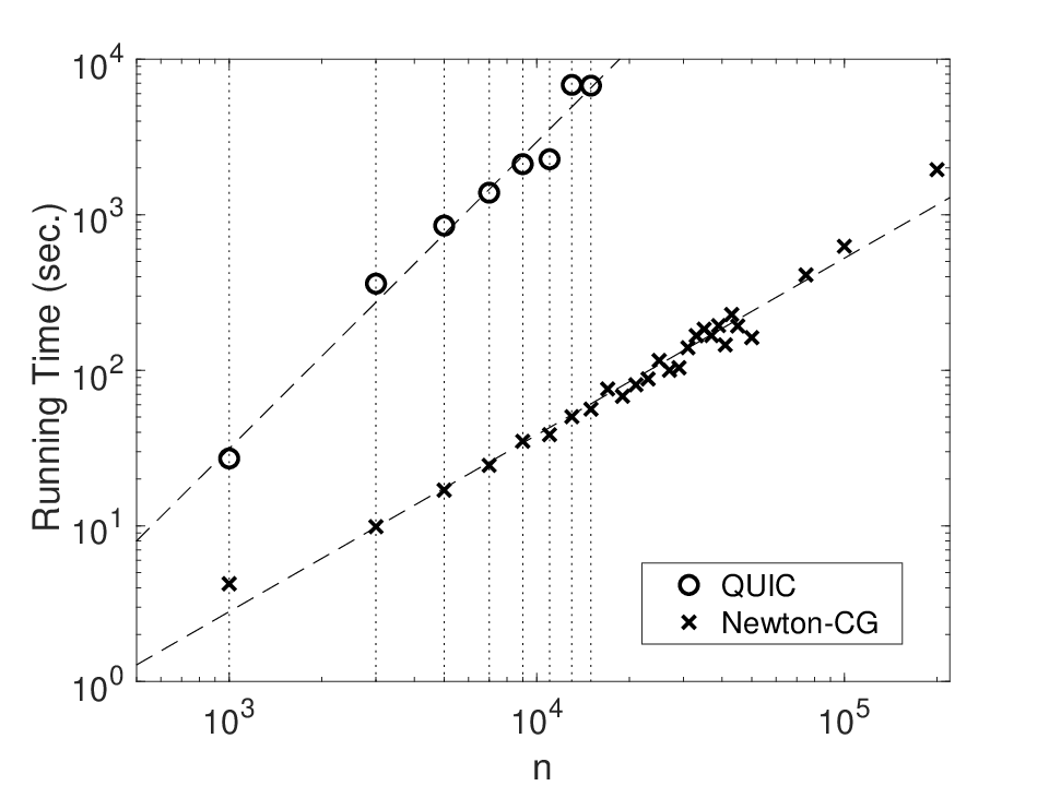
Figure 2a compares the running time of both algorithms. A log-log regression results in an empirical time complexity of $O(n^{1.1})$ for our algorithm, and $O(n^{2})$ for QUIC. The extra 0.1 in the exponent is most likely an artifact our MATLAB implementation. In either case, QUIC’s quadratic complexity limits it to $n=1.5\times 10^{4}$. By contrast, our algorithm solves an instance with $n=2\times 10^{5}$ in less than 33 minutes. The resulting solutions are extremely accurate, with optimality and feasibility gaps of less than $10^{-16}$ and $10^{-7}$, respectively.

The second case study aims to benchmark the full thresholding-MDMC procedure for sparse inverse covariance estimation on real-life graphs. The actual graphs (i.e. the sparsity patterns) for $\Sigma^{-1}$ are chosen from SuiteSparse Matrix Collection [9]—a publicly available dataset for large-and-sparse matrices collected from real-world applications. Our chosen graphs vary in size from $n=3918$ to $n=201062$, and are taken from applications in chemical processes, material science, graph problems, optimal control and model reduction, thermal processes and circuit simulations.

For each sparsity pattern $G$, we design a corresponding $\Sigma^{-1}$ as follows. For each $(i,j)\in G$, we select $(\Sigma^{-1})_{i,j}=(\Sigma^{-1})_{j,i}$ from the uniform distribution in $[-1,1]$, and then corrupt it to zero with probability $0.3$. Then, we set each diagonal to $(\Sigma^{-1})_{i,i}=1+\sum_{j}|(\Sigma^{-1})_{i,j}|$. Using this $\Sigma$, we generate $N=5000$ samples i.i.d. as $\mathbf{x}_{1},\ldots,\mathbf{x}_{N}\sim\mathcal{N}(0,\Sigma)$. This results in a sample covariance matrix $C=\frac{1}{N}\sum_{i=1}^{N}\mathbf{x}_{i}\mathbf{x}_{i}^{T}$.

We solve graphical lasso and RGL with the $C$ described above using our proposed soft-thresholding-MDMC algorithm and QUIC, in order to estimate $\Sigma^{-1}$. In the case of RGL, we assume that the graph $G$ is known a priori, while noting that 30% of the elements of $\Sigma^{-1}$ have been corrupted to zero. Our goal here is to discover the location of these corrupted elements. In all of our simulations, the threshold $\lambda$ is set so that the number of nonzero elements in the the estimator is roughly the same as the ground truth. We limit both algorithms to 3 hours of CPU time.

Figure 2b compares the CPU time of both two algorithms for this case study; the specific details are provided in Table 1. A log-log regression results in an empirical time complexity of $O(n^{1.64})$ and $O(n^{1.55})$ for graphical lasso and RGL using our algorithm, and $O(n^{2.46})$ and $O(n^{2.52})$ for the same using QUIC. The exponents of our algorithm are $\geq 1$ due to the initial soft-thresholding step, which is quadratic-time on a serial computer, but $\leq 2$ because the overall procedure is dominated by the solution of the MDMC. Both algorithms solve graphs with $n\leq 1.5\times 10^{4}$ within the allotted time limit, though our algorithm is 11 times faster on average. Only our algorithm is able to solve the estimation problem with $n\approx 2\times 10^{5}$ in a little more than an hour.

To check whether thresholding-MDMC really does solve graphical lasso and RGL, we substitute the two sets of estimators back into their original problems (1) and (5). The corresponding objective values have a relative difference $\leq 4\times 10^{-4}$, suggesting that both sets of estimators are about equally optimal. This observation verifies our claims in Theorem 2 and Corollary 3 that (1) and (5): thresholding-MDMC does indeed solve graphical lasso and RGL.

References

- [1] Ajit Agrawal, Philip Klein, and R Ravi. Cutting down on fill using nested dissection: Provably good elimination orderings. In Graph Theory and Sparse Matrix Computation, pages 31–55. Springer, 1993.
- [2] Martin S Andersen, Joachim Dahl, and Lieven Vandenberghe. Implementation of nonsymmetric interior-point methods for linear optimization over sparse matrix cones. Mathematical Programming Computation, 2(3):167–201, 2010.
- [3] Martin S Andersen, Joachim Dahl, and Lieven Vandenberghe. CVXOPT: A Python package for convex optimization. Available at cvxopt. org, 54, 2013.
- [4] Martin S Andersen, Joachim Dahl, and Lieven Vandenberghe. Logarithmic barriers for sparse matrix cones. Optimization Methods and Software, 28(3):396–423, 2013.
- [5] Onureena Banerjee, Laurent El Ghaoui, and Alexandre d’Aspremont. Model selection through sparse maximum likelihood estimation for multivariate Gaussian or binary data. Journal of Machine learning research, 9:485–516, 2008.
- [6] Richard Barrett, Michael W Berry, Tony F Chan, James Demmel, June Donato, Jack Dongarra, Victor Eijkhout, Roldan Pozo, Charles Romine, and Henk Van der Vorst. Templates for the solution of linear systems: building blocks for iterative methods, volume 43. Siam, 1994.
- [7] D. Croft, G. O’Kelly, G. Wu, R. Haw, M. Gillespie, L. Matthews, M. Caudy, P. Garapati, G. Gopinath, B. Jassal, and S. Jupe. Reactome: a database of reactions, pathways and biological processes. Nucleic acids research, 39:691–697, 2010.
- [8] Joachim Dahl, Lieven Vandenberghe, and Vwani Roychowdhury. Covariance selection for nonchordal graphs via chordal embedding. Optimization Methods & Software, 23(4):501–520, 2008.
- [9] Timothy A. Davis and Yifan Hu. The university of florida sparse matrix collection. ACM Transactions on Mathematical Software (TOMS), 38(1):1, 2011.
- [10] Steven N. Durlauf. Nonergodic economic growth. The Review of Economic Studies, 60(2):349–366, 1993.
- [11] Hilmi E. Egilmez, Eduardo Pavez, and Antonio Ortega. Graph learning from data under laplacian and structural constraints. IEEE Journal of Selected Topics in Signal Processing, 11(6):825–841, 2017.
- [12] Salar Fattahi and Somayeh Sojoudi. Graphical lasso and thresholding: Equivalence and closed-form solutions. https://arxiv.org/abs/1708.09479, 2017.
- [13] Salar Fattahi, Richard Y Zhang, and Somayeh Sojoudi. Sparse inverse covariance estimation for chordal structures. https://arxiv.org/abs/1711.09131, 2018.
- [14] Jerome Friedman, Trevor Hastie, and Robert Tibshirani. Sparse inverse covariance estimation with the graphical lasso. Biostatistics, 9(3):432–441, 2008.
- [15] Alan George and Joseph WH Liu. The evolution of the minimum degree ordering algorithm. Siam review, 31(1):1–19, 1989.
- [16] John Russell Gilbert. Some nested dissection order is nearly optimal. Information Processing Letters, 26(6):325–328, 1988.
- [17] Maxim Grechkin, Maryam Fazel, Daniela M. Witten, and Su-In Lee. Pathway graphical lasso. AAAI, pages 2617–2623, 2015.
- [18] Anne Greenbaum. Iterative methods for solving linear systems, volume 17. Siam, 1997.
- [19] Jean Honorio, Dimitris Samaras, Nikos Paragios, Rita Goldstein, and Luis E. Ortiz. Sparse and locally constant gaussian graphical models. Advances in Neural Information Processing Systems, pages 745–753, 2009.
- [20] C. J. Hsieh, M. A. Sustik, I. S. Dhillon, and P. Ravikumar. Quic: quadratic approximation for sparse inverse covariance estimation. Journal of Machine Learning Research, 15(1):2911–2947, 2014.
- [21] Cho-Jui Hsieh, Mátyás A Sustik, Inderjit S Dhillon, Pradeep K Ravikumar, and Russell Poldrack. Big & quic: Sparse inverse covariance estimation for a million variables. In Advances in neural information processing systems, pages 3165–3173, 2013.
- [22] Junzhou Huang and Tong Zhang. The benefit of group sparsity. The Annals of Statistics, 38(4):1978–2004, 2010.
- [23] Jinchao Li, Martin S Andersen, and Lieven Vandenberghe. Inexact proximal newton methods for self-concordant functions. Mathematical Methods of Operations Research, 85(1):19–41, 2017.
- [24] Stan Z. Li. Markov random field models in computer vision. European conference on computer vision, pages 351–370, 1994.
- [25] Christopher D. Manning and Hinrich Schütze. Foundations of statistical natural language processing. MIT press, 1999.
- [26] Rahul Mazumder and Trevor Hastie. Exact covariance thresholding into connected components for large-scale graphical lasso. Journal of Machine Learning Research, 13:781–794, 2012.
- [27] Nicolai Meinshausen and Peter Bühlmann. High-dimensional graphs and variable selection with the lasso. The annals of statistics, 1436–1462, 2006.
- [28] Peyman Milanfar. A tour of modern image filtering: New insights and methods, both practical and theoretical. IEEE Signal Processing Magazine, 30(1):106–128, 2013.
- [29] Sahand Negahban and Martin J. Wainwright. Joint support recovery under high-dimensional scaling: Benefits and perils of -regularization. Proceedings of the 21st International Conference on Neural Information Processing Systems, pages 1161–1168, 2008.
- [30] Yurii Nesterov. Introductory lectures on convex optimization: A basic course, volume 87. Springer Science & Business Media, 2013.
- [31] Guillaume Obozinski, Martin J. Wainwright, and Michael I. Jordan. Union support recovery in high-dimensional multivariate regression. Communication, Control, and Computing, 2008 46th Annual Allerton Conference on, pages 21–26, 2008.
- [32] Figen Oztoprak, Jorge Nocedal, Steven Rennie, and Peder A Olsen. Newton-like methods for sparse inverse covariance estimation. In Advances in neural information processing systems, pages 755–763, 2012.
- [33] Dongjoo Park and Laurence R. Rilett. Forecasting freeway link travel times with a multilayer feedforward neural network. Computer Aided Civil and Infrastructure Engineering, 14(5):357–367, 1999.
- [34] P. Ravikumar, M. J. Wainwright, G. Raskutti, and B. Yu. High-dimensional covariance estimation by minimizing -penalized log-determinant divergence. Electronic Journal of Statistics, 5:935–980, 2011.
- [35] Benjamin Rolfs, Bala Rajaratnam, Dominique Guillot, Ian Wong, and Arian Maleki. Iterative thresholding algorithm for sparse inverse covariance estimation. In Advances in Neural Information Processing Systems, pages 1574–1582, 2012.
- [36] Donald J Rose. Triangulated graphs and the elimination process. Journal of Mathematical Analysis and Applications, 32(3):597–609, 1970.
- [37] Adam J. Rothman, Peter J. Bickel, Elizaveta Levina, and Ji Zhu. Sparse permutation invariant covariance estimation. Electronic Journal of Statistics, 2:494–515, 2008.
- [38] Yousef Saad. Iterative methods for sparse linear systems, volume 82. Siam, 2003.
- [39] Somayeh Sojoudi. Equivalence of graphical lasso and thresholding for sparse graphs. Journal of Machine Learning Research, 17(115):1–21, 2016.
- [40] Eran Treister and Javier S Turek. A block-coordinate descent approach for large-scale sparse inverse covariance estimation. In Advances in neural information processing systems, pages 927–935, 2014.
- [41] Lieven Vandenberghe, Martin S Andersen, et al. Chordal graphs and semidefinite optimization. Foundations and Trends® in Optimization, 1(4):241–433, 2015.
- [42] Martin J Wainwright. Sharp thresholds for high-dimensional and noisy sparsity recovery using -constrained quadratic programming (lasso). IEEE transactions on information theory, 55(5):2183–2202, 2009.
- [43] Eunho Yang, Aurélie C. Lozano, and Pradeep K. Ravikumar. Elementary estimators for graphical models. Advances in neural information processing systems, pages 2159–2167, 2014.
- [44] Mihalis Yannakakis. Computing the minimum fill-in is NP-complete. SIAM Journal on Algebraic Discrete Methods, 2(1):77–79, 1981.
- [45] Ming Yuan and Yi Lin. Model selection and estimation in the Gaussian graphical model. Biometrika, pages 19–35, 2007.
Appendix A Restricted graphical Lasso and MDMC
Our aim is to elucidate the connection between the RGL and MDMC problem under the assumption that the regularization coefficients are chosen to be large, i.e., when a sparse solution for the RGL is sought. Recall that RGL is formulated as follows