The generation of helical magnetic field in a viable scenario of Inflationary Magnetogenesis

Cosmic magnetic fields have been detected from planetery scales [1] to galaxy clusters scales [2, 3, 4]. $\gamma$-ray observations of Blazars suggest their presence in the voids as well [5, 6]. However the origin of these fields do not have a fully satisfactory explanation. Astrophysical scenarios [7, 8, 9, 10, 11] for generating these fields involve battery effects to create a seed field which is later amplified to the observed strength by the dynamo action [12, 13, 14, 15]. However, the presence of coherent magnetic fields in void regions favor primordial scanarios of generation. Several possible scenarios for this have been suggested in literature [16, 17, 18, 19, 20, 21, 22, 23, 24, 25, 26, 27, 28, 29, 30, 31, 32, 33, 34, 35, 36, 37] (for reviews, see [38, 39, 40, 41, 42]).

Inflationary magnetogenesis is one of the possible scenarios to generate fields that are coherent over large scales. However the generation of magnetic field during inflation in the standard physics is not possible due to the conformal invariance of the electromagnetic field [43]. A breaking of conformal invariance is necessary. This has been done in many models by taking a time dependent function coupled with the kinetic energy term of the electromagnetic (EM) field. This time dependent coupling term can arise through the coupling between inflaton field and EM field (Ratra model) [18] or by taking a non-minimal coupling of the EM field to the gravitational field [16].

Although Ratra model generates sufficient strength of the magnetic field, it potentially suffers from strong coupling and back-reaction problems [44]. These problems have been resolved by further modification of the Ratra model [29, 31, 45]. In Ref. [45], to resolve these problems $f$ is assumed to increase during inflation and decrease back to its initial value post inflation. Firstly this behaviour of $f$ circumvents the strong coupling problem. Moreover, for a small enough inflationary and reheating scales, the model also does not suffer from the back-reaction problem. Indeed demanding no back-reaction post inflation, bounds on the inflationary scale and reheating scale has been obtained. The generated magnetic field strength in this model can also explain the magnetic field strength suggested by $\gamma$-ray observation, below a certain reheating scale.

In the model discussed above, the generated magnetic field is of non-helical nature. In this paper we look at the possible generation of helical magnetic fields. The non-linear evolution of magnetic field in helical case differs from non-helical one. Due to the helicity conservation, the magnetic field strength decreases at a slower rate and the correlation length increases at a higher rate compared to the non-helical case. Helicity conservation gives us a more optimistic evolution of the magnetic field and this can relax the bound on the reheating scale given in [45] further.

Moreover, it has been claimed in the literature that gamma ray observations of the Blazars indicate the presence of helical magnetic field in intergalactic medium [46, 47]. To generate helical magnetic field, we add a parity breaking term in the Electromagnetic action. We also compare our generated magnetic field strength with the constraints from $\gamma$-ray observation.

This paper is organised as follows. In section II we discuss the generation of helical magnetic field during inflation. Section III discusses the generation of the field post inflation to reheating and we obtain a relation between inflationary scale and reheating scale by demanding no back-reaction post inflation. Section IV incorporates the nonlinear evolution of magnetic field and its correlation length after generation. Results of our model are also given there. In section V, we compare our results with the $\gamma$-ray observation. Our conclusions are presented in VI.

We start with the action for the electromagnetic field in which the conformal invariance is explicitly broken by introducing a time dependent function $f^{2}$ multiplying $F^{\mu\nu}F_{\mu\nu}$ in the action. To generate helical magnetic field, we also add a $f^{2}{F_{\mu\nu}}{\tilde{F}^{\mu\nu}}$ in the action. Thus we take the action to be of the form,

	$\displaystyle S$	$\displaystyle=-\int\sqrt{-g}d^{4}x[\frac{f^{2}(\phi)}{16\pi}\left({F_{\mu\nu}}{F^{\mu\nu}}+{F_{\mu\nu}}{\tilde{F}^{\mu\nu}}\right)+j^{\mu}A_{\mu}]$			(1)
		$\displaystyle-\int\sqrt{-g}d^{4}x\Big[\frac{1}{2}\partial^{\nu}\phi\partial_{\nu}\phi+V(\phi)\Big]$

Here $F_{\mu\nu}=\partial_{\mu}A_{\nu}-\partial_{\nu}A_{\mu}$ and $\tilde{F}^{\mu\nu}=(1/2)\epsilon^{\mu\nu\alpha\beta}F_{\alpha\beta}$, where $A_{\mu}$ is the EM 4-potential and $\epsilon^{\mu\nu\alpha\beta}$ is fully antisymmetric tensor defined as $\epsilon^{\mu\nu\alpha\beta}=1/\sqrt{-g}~\eta^{\mu\nu\alpha\beta}$. $\eta^{\mu\nu\alpha\beta}$ is levi-civita symbol whose values are $\pm 1$ only. The term $j^{\mu}A_{\mu}$ represents the interaction where $j^{\mu}$ is the four current density. Remaining part of the action incorporates the evolution of the inflaton field. In this paper we adopt the following nomenclature. Greek indices $\mu,\nu....$ are for space-time coordinates and Roman indices $i,j,k....$ are for spatial coordinates. Our metric convention is $g_{\mu\nu}=diag(-,+,+,+)$. For further analysis we assume negligible free charge density during inflation. Hence, we neglect the interaction term. To obtain the equation of motion of 4-potential $A_{\mu}$ we vary the action with respect to the $A_{\mu}$.

	$\displaystyle[f^{2}\left(F^{\mu\nu}+\tilde{F}^{\mu\nu}\right)]_{;\nu}$	$\displaystyle=0$
	$\displaystyle\frac{1}{\sqrt{-g}}\frac{\partial}{\partial x^{\nu}}\Bigg[\sqrt{-g}f^{2}(\phi)\Big(g^{\mu\alpha}g^{\nu\beta}F_{\alpha\beta}$
	$\displaystyle+\frac{1}{\sqrt{-g}}\eta^{\mu\nu\alpha\beta}F_{\alpha\beta}\Big)\Bigg]$	$\displaystyle=0$		(2)

Varying the action with respect to scalar field we obtain the equation governing the evolution of the scalar field as

	$\displaystyle\frac{1}{\sqrt{-g}}\frac{\partial}{\partial x^{\nu}}\Big[\sqrt{-g}g^{\mu\nu}\partial_{\mu}\phi\Big]-\frac{dV}{d\phi}$	$\displaystyle=\frac{f}{2}\frac{df}{d\phi}\Big(F_{\mu\nu}F^{\mu\nu}$
		$\displaystyle+F_{\mu\nu}\tilde{F}^{\mu\nu}\Big)$		(3)

Here EM field is assumed to be a test field. Hence, it will not affect the geometry of spacetime. In the inflationary era the universe is dominated by scalar field $\phi$ which is a time dependent homogeneous field. We work in a frame work of homogeneous and isotropic universe, described by the FRW line element.

	$\displaystyle ds^{2}$	$\displaystyle=$	$\displaystyle-dt^{2}+a^{2}(t)[dx^{2}+dy^{2}+dz^{2}]$		(4)
		$\displaystyle=$	$\displaystyle a^{2}(\eta)[-d\eta^{2}+dx^{2}+dy^{2}+dz^{2}]$

In this new coordinate system $(\eta,x,y,z)$, we can define fundamental observers with four velocity $(\frac{1}{a},0,0,0)$. It is convenient to work in Coulomb gauge,

$$\partial_{j}A^{j}=0\quad,\quad A_{0}=0$$

For $\mu=i$, Eq. (2) is

$$A_{i}^{\prime\prime}+2\frac{f^{\prime}}{f}\left(A_{i}^{\prime}+\eta_{ijk}\partial_{j}A_{k}\right)-a^{2}\partial_{j}\partial^{j}A_{i}=0$$

(5)

Here prime(’) denotes derivative with respect to $\eta$ and $\partial^{j}$ is defined as $\partial^{j}\equiv g^{jk}\partial_{k}=a^{-2}\delta^{jk}\partial_{k}$. $\eta_{ijk}$ represents the three dimensional levi-civita symbol. To quantize the EM field, we calculate the conjugate momentum ($\Pi^{i}$)of $A^{i}$ field, promote these fields to operators and impose the canonical quantization condition,

$\displaystyle\Pi^{i}=\frac{\delta L}{\delta\dot{A}_{i}},$

(6)

$\displaystyle[A^{i},\Pi_{j}]=i\int\frac{d^{3}k}{2\pi^{3}}e^{\vec{k}\cdot(\vec{x}-\vec{y})}P^{i}_{j}(k).$

(7)

Here $P^{i}_{j}=\delta^{i}_{j}-\delta_{jm}(k^{i}k^{m}/k^{2})$ is used to ensure the coulomb gauge condition. We fourier transform $A_{i}$ using the momentum space operators ($b_{\lambda}$ and $b_{\lambda}^{\dagger}$).

	$\displaystyle A^{i}(\vec{x},\eta)$	$\displaystyle=\sqrt{4\pi}\int\frac{d^{3}k}{2\pi^{3}}\sum_{\lambda=1,2}\epsilon^{i}_{\lambda}\Big[A_{\lambda}(k,\eta)b_{\lambda}(\vec{k})e^{i\vec{k}\cdot\vec{x}}$
		$\displaystyle+A_{\lambda}^{*}(k,\eta)b^{\dagger}_{\lambda}(\vec{k})e^{-i\vec{k}\cdot\vec{x}}\Big].$		(8)

Here $\epsilon^{i}_{\lambda}$ represents the polarisation vector which can be written in terms of the 3-dimensional orthonormal unit vectors as

$\displaystyle\epsilon^{i}_{\lambda}=\frac{\hat{\epsilon}^{i}_{\lambda}}{a}~~,~~\epsilon^{i}_{3}=\frac{\hat{k}}{a}$

(9)

Here $\hat{\epsilon}^{i}_{\lambda}$ are unit 3-vectors, orthogonal to $\hat{k}$ and each other. It is useful to define a new variable $\bar{A}_{\lambda}$ as, $\bar{A}_{\lambda}=aA_{\lambda}(k,\eta)$. Substituting Eq.(8) in Eq.(5).

$$\sum_{\lambda}b_{\lambda}\Big[\hat{\epsilon}_{i\lambda}\left(\bar{A}_{\lambda}^{\prime\prime}+2\frac{f^{\prime}}{f}\bar{A}_{\lambda}^{\prime}+k^{2}\bar{A}_{\lambda}\right)+\frac{2f^{\prime}}{f}\eta_{ijm}\hat{\epsilon}_{m\lambda}k_{j}\bar{A}_{\lambda}\Big]=0$$

(10)

To simplify this equation further let’s choose a different set of basis vector defined as $\hat{\epsilon}_{+}=(\hat{\epsilon}_{1}+i\hat{\epsilon}_{2})/2$ and $\hat{\epsilon}_{-}=(\hat{\epsilon}_{1}-i\hat{\epsilon}_{2})/2$. In terms of these new basis vectors, $\sum_{\lambda}\bar{A}_{\lambda}\hat{\epsilon}_{\lambda}b_{\lambda}=\bar{A}_{+}\hat{\epsilon}_{+}b_{+}+\bar{A}_{-}\hat{\epsilon}_{-}b_{-}$. This set of basis vectors are known as the helicity basis. Then Eq.(10) reduces to

$$\bar{A}_{h}^{\prime\prime}+2\frac{f^{\prime}}{f}\left(\bar{A}_{h}^{\prime}+hk\bar{A}_{h}\right)+k^{2}\bar{A}_{h}=0$$

(11)

Here $h=\pm 1$ represents the helicity sign. The equation of motion in terms of $\mathcal{A}_{h}=f\bar{A}_{h}(k,\eta)$ turns out to be,

$$\mathcal{A}_{h}^{\prime\prime}(k,\eta)+\Big(k^{2}-\frac{f^{\prime\prime}}{f}+2hk\frac{f^{\prime}}{f}\Big)\mathcal{A}_{h}(k,\eta)=0$$

(12)

Before we solve the above equation for a particular $f(\phi)$, it will be of interest to calculate the energy density of the EM field. To do this we calculate the energy momentum tensor of the EM field.

	$\displaystyle T_{\mu\nu}$	$\displaystyle\equiv-\frac{2}{\sqrt{-g}}\frac{\delta\sqrt{-g}\mathcal{L}}{\delta g^{\mu\nu}}$
		$\displaystyle=\frac{f^{2}}{4\pi}\left[g^{\alpha\beta}F_{\mu\alpha}F_{\nu\beta}-g_{\mu\nu}\frac{F^{\alpha\beta}F_{\alpha\beta}}{4}\right]$		(13)

We define the electric and magnetic field four vectors as $B^{\mu}\equiv\tilde{F}^{\mu\nu}u_{\nu}$ and $E^{\mu}\equiv F^{\mu\nu}u_{\nu}$. For the observer $u^{\mu}=(1/a,0,0,0)$, the time component of these vectors are zero. The spatial components are given by $B_{i}=(1/a)\eta_{ijk}\delta^{jm}\delta^{kn}\partial_{m}A_{n}$ and $E_{i}=-(1/a)\partial_{\eta}A_{i}$. Then the EM energy densities of ground state measured by the observer with 4-velocity $u^{\mu}=(1/a,0,0,0)$ are given by,

$\displaystyle\rho_{B}=\langle 0|T^{B}_{\mu\nu}u^{\mu}u^{\nu}|0\rangle\quad\text{and}\quad\rho_{E}=\langle 0|T^{E}_{\mu\nu}u^{\mu}u^{\nu}|0\rangle,$

(14)

where we have separated the total energy density into the magnetic part and the electric part. We express these parts in terms of $A^{i}$ as,

	$\displaystyle\rho_{B}$	$\displaystyle=$	$\displaystyle\langle 0|\frac{f^{2}}{8\pi}\left[\partial_{i}A_{n}\partial_{j}A_{l}\left(g^{ij}g^{nl}-g^{il}g^{nj}\right)\right]|0\rangle$		(15)
		$\displaystyle=$	$\displaystyle\langle 0|\frac{f^{2}}{8\pi}B^{i}B_{i}|0\rangle$
	$\displaystyle\text{and}\quad\rho_{E}$	$\displaystyle=$	$\displaystyle\langle 0|\frac{f^{2}}{8\pi}\left[A^{\prime}_{i}A^{\prime}_{j}g^{ij}\right]|0\rangle$		(16)
		$\displaystyle=$	$\displaystyle\langle 0|\frac{f^{2}}{8\pi}E^{i}E_{i}|0\rangle$

After substituting $A_{i}$ from Eq.(8) into Eq.(15) and Eq.(16), and using the helicity basis, we reduce the energy densities in terms of $\mathcal{A_{+}}$ and $\mathcal{A_{-}}$.

	$\displaystyle\rho_{B}\equiv\int\frac{dk}{k}\frac{d\rho_{B}(k,\eta)}{d\ln k}$	$\displaystyle=$	$\displaystyle\int\frac{dk}{k}\frac{1}{(2\pi)^{2}}\frac{k^{5}}{a^{4}}\Big(|\mathcal{A}_{+}(k,\eta)|^{2}$		(17)
		$\displaystyle+$	$\displaystyle|\mathcal{A}_{-}(k,\eta)|^{2}\Big)$
	$\displaystyle\rho_{E}\equiv\int\frac{dk}{k}\frac{d\rho_{E}(k,\eta)}{d\ln k}$	$\displaystyle=$	$\displaystyle\int\frac{dk}{k}\frac{f^{2}}{(2\pi)^{2}}\frac{k^{3}}{a^{4}}\Bigg(\left|\Big[\frac{\mathcal{A}_{+}(k,\eta)}{f}\Big]^{\prime}\right|^{2}$		(18)
		$\displaystyle+$	$\displaystyle\left|\Big[\frac{\mathcal{A}_{-}(k,\eta)}{f}\Big]^{\prime}\right|^{2}\Bigg)$

In deriving the above expressions we have used the following properties,

$\displaystyle b_{h}|0\rangle=0~~~~\langle 0|b_{h}(\vec{k})b^{\dagger}_{h^{\prime}}(\vec{k^{\prime}})|0\rangle=(2\pi)^{3}\delta_{hh^{\prime}}\delta^{3}(\vec{k}-\vec{k^{\prime}})$

In our analysis, we work with the spectral energy densities of magnetic and electric fields given by $(d\rho_{B}(k,\eta)/d\ln k)$ and $(d\rho_{E}(k,\eta)/d\ln k)$ respectively. These spectral densities represent the energy contained in logarithmic interval in k-space.

We now turn to calculation of the magnetic and electric spectral energy densities for a particular type of coupling function. Let us assume the form of the coupling function to be a simple power law as,

$$f_{1}(a)=f_{i}\left(\frac{a}{a_{i}}\right)^{\alpha}.$$

(19)

We assume that during inflation $f(\phi)$ has a form such that $f$ evolves with $a$ as given in (19). Here $a_{i}$ represents the value of scale factor at the beginning of inflation and $\alpha$ is a real constant. By assuming the background to be purely de-sitter during inflation ($a\propto\eta^{-1}$), we get the following

$$\frac{f_{1}^{\prime\prime}}{f_{1}}=\frac{\alpha(\alpha+1)}{\eta^{2}}.$$

(20)

For this form of coupling function Eq.(12) reduces to

$$\mathcal{A}_{h}^{\prime\prime}(k,\eta)+\Big(k^{2}-\frac{\alpha(\alpha+1)}{\eta^{2}}-2hk\frac{\alpha}{\eta}\Big)\mathcal{A}_{h}(k,\eta)=0.$$

(21)

To solve Eq.(21), we rewrite it by defining some new variables, $\mu^{2}\equiv\alpha(\alpha+1)+\frac{1}{4},\quad\kappa\equiv i\alpha h,\quad z\equiv 2ik\eta$. Then the equation takes the form,

$$\frac{\partial^{2}\mathcal{A}_{h}(k,\eta)}{\partial z^{2}}+\left[\frac{1}{z^{2}}\left(\frac{1}{4}-\mu^{2}\right)+\frac{\kappa}{z}-\frac{1}{4}\right]\mathcal{A}_{h}(k,\eta)=0.$$

(22)

The solutions of this equation are Whittaker functions [48],

$$\mathcal{A}_{h}=c_{1}W_{\kappa,\mu}(z)+c_{2}W_{-\kappa,\mu}(-z).$$

(23)

To determine the coefficients $c_{1}$ and $c_{2}$, we have matched the solution with the bunch davies vacuum in the sub horizon limit $|-k\eta|>>1$, $\mathcal{A}_{h}=\frac{e^{-ik\eta}}{\sqrt{2k}}$. After matching we get,

$$\mathcal{A}_{h}=\frac{e^{\frac{i\pi\kappa}{2}}}{\sqrt{2k}}W_{\kappa,\mu}(z)=\frac{e^{\frac{-h\pi\alpha}{2}}}{\sqrt{2k}}W_{i\alpha h,\alpha+\frac{1}{2}}(2ik\eta)$$

At the end of the inflation, all the modes of cosmological interest will be outside the horizon. To get the spectral magnetic energy density of these modes, we need to write the above expression in the super horizon limit.

	$\displaystyle\mathcal{A}_{h}$	$\displaystyle=\frac{C_{h}}{\sqrt{2k}}\Big[(-k\eta)^{-\alpha}+h(-k\eta)^{-\alpha+1}\Big]+$
		$\displaystyle~~~\frac{D_{h}}{\sqrt{2k}}\Big[(-k\eta)^{1+\alpha}-\frac{h\alpha}{1+\alpha}(-k\eta)^{2+\alpha}\Big]$		(24)

Here

	$\displaystyle C_{h}$	$\displaystyle=e^{\frac{-h\pi\alpha}{2}}\frac{(-2i)^{-\alpha}\Gamma(1+2\alpha)}{\Gamma(1+\alpha+ih\alpha)},$
	$\displaystyle D_{h}$	$\displaystyle=e^{\frac{-h\pi\alpha}{2}}\frac{(-2i)^{1+\alpha}\Gamma(-1-2\alpha)}{\Gamma(-\alpha-ih\alpha)}.$		(25)

Substituting Eq.(24) into Eq.(17) the spectral magnetic energy density comes out to be,

	$\displaystyle\frac{d\rho_{B}}{d\ln k}$	$\displaystyle=$	$\displaystyle\frac{1}{8\pi^{2}}H_{f}^{4}\Big[\left(|C_{+}|^{2}+|C_{-}|^{2}\right)(-k\eta)^{-2\alpha+4}$		(26)
		$\displaystyle+$	$\displaystyle\left(|D_{+}|^{2}+|D_{-}|^{2}\right)(-k\eta)^{2\alpha+6}\Big].$

Similarly the spectral electric energy density is given by,

	$\displaystyle\frac{d\rho_{E}}{d\ln k}$	$\displaystyle=$	$\displaystyle\frac{1}{8\pi^{2}}H_{f}^{4}\Big[\left(|C_{+}|^{2}+|C_{-}|^{2}\right)(-k\eta)^{-2\alpha+4}$		(27)
		$\displaystyle+$	$\displaystyle\left(|D_{+}|^{2}+|D_{-}|^{2}\right)(1+2\alpha)^{2}(-k\eta)^{2\alpha+4}\Big].$

For the expressions in Eq.(26) and Eq.(27), we have only kept the dominant terms.

The reason of two branches in the above expressions is that $\alpha$ can be positive or negative. In the magnetic field spectrum the first branch dominates when $\alpha>1/2$ and the other branch dominates when $\alpha<1/2$. For the electric field spectrum the first branch dominates when $\alpha>-1/2$ and the other branch dominates when $\alpha<-1/2$. There are two possible value of $\alpha$ (namely, $\alpha=2,-3$) for which the magnetic field spectrum is scale invariant.

For the case $\alpha=-3$, when the magnetic field is scale invariant the electric field spectrum diverges as $(-k\eta)^{-2}$. This implies that the electric field energy density may overshoot the inflaton energy density during inflation in this case and our assumption of EM field being a test field would no longer be valid. This problem is known as the back-reaction problem [44].

However, for the case $\alpha=2$, both the magnetic and electric field spectrum are scale invariant, and this avoids the back reaction problem. For this case the coupling function $f$ is proportional to $a^{2}$, which means that $f$ will be very large at the end of inflation compared to its initial value. If we assume that $f$ becomes a constant at the end of inflation, then the effective EM charge $e_{f}=1/f^{2}$. Suppose we demand that at the end of inflation $e_{f}$ should have the observed value, then it will be very large at the beginning of inflation. Due to this large value of $e_{f}$, our perturbative analysis of field theory would no longer be valid. This problem is known as strong coupling problem [44]. On the other hand, if $e_{f}$ has the observed value at the beginning of inflation, it will have a very small value at the end of inflation, avoiding the strong coupling problem. This case is further explored in the next section.

The branch $\alpha=2$ is also preferred, as we discussed in detail in Ref. [45], because it evades the constraints imposed by the possibility of increased conductivity due to the Schwinger effect [31]. The magnetic energy spectrum at the end of inflation for $\alpha=2$,

$\displaystyle\frac{d\rho_{B}}{d\ln k}$

$\displaystyle\approx\frac{9~e^{4\pi}}{320\pi^{3}}H_{f}^{4}$

(28)

We note that this value is larger than the non-helical case by a factor of $(e^{4\pi}/80\pi)\approx 10^{3}$.

As discussed in the last section, there are two possible scenarios for obtaining a scale invariant magnetic spectrum. The case in which $f$ is increasing during inflation avoids the back-reaction problem. Moreover if we assume that $f$ begins with a value of unity at the onset of inflation and increases during the inflationary phase, there will be no strong coupling problem. At end of inflation, however, the EM field will be very weakly coupled to the charged particles as $f$ is much larger than unity. We address this issue in [45] by postulating that from the end of inflation onwards $f$ decreases and attains a value of unity at reheating and remains unity thereafter. This ensures that EM action is again in the standard conformally invariant form after the reheating era. Thus the deviation from the standard form is onset of inflation to the reheating.

We assume the universe to be matter dominated from the end of inflation to reheating. We consider $\alpha>1/2$ for further analysis. In this era the evolution of the scale factor is as follows,

$$a=\frac{a_{f}^{3}H_{f}^{2}}{4}\left(\eta+\frac{3}{a_{f}H_{f}}\right)^{2}$$

and the coupling function $f$ is assumed to evolve as

$\displaystyle f\propto\left(\frac{a}{a_{f}}\right)^{-\beta}$

Here $a_{f}$ is the value of scale factor at the end of inflation. We calculate the constant of proportionality by demanding the continuity of $f$ at the end of inflation.

$\displaystyle f_{2}=f_{i}\left(\frac{a_{f}}{a_{i}}\right)^{\alpha}\left(\frac{a}{a_{f}}\right)^{-\beta}$

To estimate the EM energy densities in this era, we need to solve Eq.(21) for this new coupling function. Solution is given by,

$$\mathcal{A}_{2h}=d_{1}M_{2i\beta h,-(2\beta+\frac{1}{2})}(2ik\zeta)+d_{2}M_{2i\beta h,2\beta+\frac{1}{2}}(2ik\zeta)$$

(29)

Here $\zeta=\eta+3/(a_{f}H_{f})$ and $M_{2i\beta h,-(2\beta+\frac{1}{2})}(2ik\zeta)$ represents the second kind of whittaker function [48]. To calculate $d_{1}$ and $d_{2}$, we need the above expression in the super horizon limit. In this limit Eq.(29) becomes,

	$\displaystyle\mathcal{A}_{2h}$	$\displaystyle=d_{1}(2i)^{-2\beta}\left[(k\zeta)^{-2\beta}-h(k\zeta)^{-2\beta+1}\right]$
		$\displaystyle+d_{2}(2i)^{2\beta+1}\left[(k\zeta)^{2\beta+1}+\frac{2h\beta}{1+2\beta}(k\zeta)^{2\beta+2}\right]$

and,

	$\displaystyle\bar{A}_{2h}=\frac{\mathcal{A}_{2h}}{f_{2}}$	$\displaystyle=\left(\frac{k}{H_{f}}\right)^{-2\beta}\Bigg(d_{3}\left(1-h(k\zeta)\right)$
		$\displaystyle+d_{4}\left((k\zeta)^{4\beta+1}+\frac{2h\beta}{1+2\beta}(k\zeta)^{4\beta+2}\right)\Bigg)$		(30)

Here $d_{3}$ and $d_{4}$ are two new constants. They can be expressed in terms of $d_{1}$ and $d_{2}$. We demand that at the end of the inflation both $\bar{A}_{h}$, $\bar{A}_{2h}$ and their derivatives have to be matched. After matching we get,

$\displaystyle d_{3}$

$\displaystyle=\frac{C_{h}}{\sqrt{2k}}\left(\frac{k}{H_{f}}\right)^{-\alpha+2\beta}\left(1+3h\left(\frac{k}{a_{f}H_{f}}\right)\right)$

and

	$\displaystyle d_{4}$	$\displaystyle=\frac{C_{h}}{\sqrt{2k}}\left(\frac{k}{H_{f}}\right)^{-\alpha+2\beta}\frac{3h^{2}}{2(4\beta+1)}\left(\frac{2k}{a_{f}H_{f}}\right)^{-4\beta+1}$
		$\displaystyle\left(1-\frac{2h\beta}{1+2\beta}\frac{4\beta+2}{4\beta+1}\left(\frac{2k}{a_{f}H_{f}}\right)\right)^{-1}$

In $d_{3}$ and $d_{4}$ expressions, we only take the contribution of dominant terms. Energy densities after inflation evolve as

	$\displaystyle\frac{d\rho_{B}}{d\ln k}$	$\displaystyle=\frac{C_{1}}{8\pi^{2}}\frac{k^{4}}{a^{4}}f_{2}^{2}(a)\left(\frac{k}{H_{f}}\right)^{-2\alpha}\Bigg(1+\frac{9}{4(4\beta+1)^{2}}$
		$\displaystyle\left(\frac{2k}{a_{f}H_{f}}\right)^{-8\beta+2}\left(\frac{2k}{aH}\right)^{8\beta+2}+\frac{3h^{2}}{(4\beta+1)}$
		$\displaystyle\left(\frac{2k}{a_{f}H_{f}}\right)^{-4\beta+1}\left(\frac{2k}{aH}\right)^{4\beta+1}\Bigg)$

	$\displaystyle\frac{d\rho_{E}}{d\ln k}$	$\displaystyle=\frac{1}{8\pi^{2}}\frac{k^{4}}{a^{4}}f_{2}^{2}(a)\left(\frac{k}{H_{f}}\right)^{-2\alpha}\Bigg(C_{1}+\frac{9}{4}C_{1}$
		$\displaystyle\left(\frac{2k}{a_{f}H_{f}}\right)^{-8\beta+2}\left(\frac{2k}{aH}\right)^{8\beta}+3C_{2}$
		$\displaystyle\left(\frac{2k}{a_{f}H_{f}}\right)^{-4\beta+1}\left(\frac{2k}{aH}\right)^{4\beta}\Bigg)$

Here $C_{1}=\left|C_{+}\right|^{2}+\left|C_{-}\right|^{2}$ and $C_{2}=\left|C_{+}\right|^{2}-\left|C_{-}\right|^{2}$. At the end of inflation, the first term inside the bracket in the expressions of $d\rho_{B}/d\ln k$ dominates for all the modes outside the horizon and gives a scale invariant magnetic field spectrum for $\alpha=2$. As $f$ decreases post inflation, this term also decreases and becomes very small at reheating. Although the second and third term are very small compared to the first term for the mode $k_{i}=a_{i}H_{f}$ at the end of inflation, the contribution from these terms compared to the first term increases as $f$ decreases post inflation. Consequently, the second and third term overshoot the first term before reheating. The second term is $36/((4\beta+1)^{2}a_{f}^{4})\times(a_{r}/a_{f})^{4\beta+1}$ times larger than the first term and $6/((4\beta+1)a_{f}^{2})\times(a_{r}/a_{f})^{2\beta+1/2}$ times larger than the third term at reheating for the mode which exit the horizon at the beginning of inflation ($k_{i}=a_{i}H_{f}$). It is even larger for all other modes of interest. After taking the contribution of the dominant term at reheating in the above expressions, we get the following expression for EM energy densities at reheating,

	$\displaystyle\frac{d\rho_{B}}{d\ln k}\Bigg|_{r}$	$\displaystyle=\frac{9}{32\pi^{2}}\frac{k^{4}}{a_{r}^{4}}f_{2}^{2}(a_{r})\left(\frac{k}{H_{f}}\right)^{-2\alpha}C_{1}$
		$\displaystyle\frac{1}{(4\beta+1)^{2}}\left(\frac{2k}{a_{f}H_{f}}\right)^{-8\beta+2}\left(\frac{2k}{a_{r}H_{r}}\right)^{8\beta+2}$		(31)

	$\displaystyle\frac{d\rho_{E}}{d\ln k}\Bigg|_{r}$	$\displaystyle=\frac{9}{32\pi^{2}}\frac{k^{4}}{a_{r}^{4}}f_{2}^{2}(a_{r})\left(\frac{k}{H_{f}}\right)^{-2\alpha}C_{1}$
		$\displaystyle\left(\frac{2k}{a_{f}H_{f}}\right)^{-8\beta+2}\left(\frac{2k}{a_{r}H_{r}}\right)^{8\beta}$		(32)

Here $a_{r}$ and $H_{r}$ are the scale factor and Hubble parameter at reheating respectively.

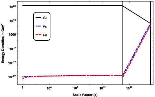
Fig. (1) shows the evolution of EM and the inflaton energy densities with the scale factor, both during and after inflation. From Fig.(1) one can see that EM energy densities are increasing after inflation. It is necessary that EM energy density does not overshoot the energy density of the universe before the coupling function $f$ reaches to its pre-inflationary value. Since EM energy density has a monotonically increasing behaviour, if $\rho_{E}+\rho_{B}<\rho_{\phi}$ is satisfied at reheating, it will be valid throughout the post inflationary era prior to reheating. The total EM energy density at reheating is,

	$\displaystyle\rho_{E}+\rho_{B}\Big|_{r}$	$\displaystyle=\int_{a_{i}H_{f}}^{k_{r}}d\ln k\left(\frac{d\rho_{E}(k,\eta)}{d\ln k}\Big|_{r}+\frac{d\rho_{B}(k,\eta)}{d\ln k}\Big|_{r}\right)$
		$\displaystyle=\int_{a_{i}H_{f}}^{k_{r}}d\ln k\Bigg[\frac{9}{32\pi^{2}}\frac{k^{4}}{a_{r}^{4}}f_{2}^{2}(a_{r})C_{1}\left(\frac{k}{H_{f}}\right)^{-2\alpha}\left(\frac{2k}{a_{f}H_{f}}\right)^{-8\beta+2}\left(\frac{2k}{a_{r}H_{r}}\right)^{8\beta}\left(1+\frac{1}{(4\beta+1)^{2}}\left(\frac{2k}{a_{r}H_{r}}\right)^{2}\right)\Bigg]$
		$\displaystyle=\frac{9}{32\pi^{2}}\frac{f_{2}^{2}(a_{r})}{a_{r}^{4}}C_{1}\left(\frac{k_{r}}{H_{f}}\right)^{-2\alpha}\left(\frac{2k_{r}}{a_{f}H_{f}}\right)^{-8\beta+2}\left(\frac{2k_{r}}{a_{r}H_{r}}\right)^{8\beta}k_{r}^{4}\left(\frac{1}{6-2\alpha}+\frac{1}{(8-2\alpha)(4\beta+1)^{2}}\left(\frac{2k_{r}}{a_{r}H_{r}}\right)^{2}\right)$		(33)

For further analysis we have used two new variable defined as,

$$N=\ln\left(\frac{a_{f}}{a_{i}}\right)~~~~~~\text{and}~~~~~N_{r}=\ln\left(\frac{a_{r}}{a_{f}}\right)$$

After substituting $k_{r}=a_{r}H_{r}=a_{f}H_{f}e^{-N_{r}/2}$ in Eq.(33) and using the definition of $N$ and $N_{r}$, we get

$\displaystyle\rho_{E}+\rho_{B}\Big|_{r}$

$\displaystyle=C_{3}H_{f}^{4}e^{\alpha(2N+N_{r})-7N_{r}}$

(34)

Here

$$C_{3}=\frac{9C_{1}}{8\pi^{2}}\left(\frac{1}{6-2\alpha}+\frac{4}{(8-2\alpha)(4\beta+1)^{2}}\right).$$

In the above expression, we also use $\beta=\alpha N/N_{r}$ which is obtained by demanding $f(a_{r})=1$.

In order that $\rho_{E}+\rho_{B}|_{r}<\rho_{\phi}|_{r}$, we require

$\displaystyle 2\alpha(N+N_{r})-(7+\alpha)N_{r}<\ln\left(\frac{\pi^{2}g_{r}}{30C_{3}}\right)-4\ln\frac{H_{f}}{T_{r}}.$

(35)

Here we use $\rho_{\phi}|_{r}=g_{r}(\pi^{2}/30)T_{r}^{4}$ where $T_{r}$ and $g_{r}$ represent reheating temperature and relativistic degree of freedom, respectively, at reheating. We have several variables in the above expression but they are all not independent. To reduce the expression in terms of the minimum number of variables (independent variables), we use the following constraint.

From the isotropy of the cosmic microwave background radiation, we find the following relation.

$\displaystyle N+N_{r}$

$\displaystyle>66.9-\ln\left(\frac{T_{r}}{H_{f}}\right)-\frac{1}{3}\ln\frac{g_{r}}{g_{0}}.$

(36)

Here, $g_{0}$ is the relativistic degree of freedom in the universe at present. The above relation has been derived from the fact that the present observable universe has to be inside the Hubble radius at the beginning of inflation. In the above expression, we also assume a radiation dominated era from reheating till today.

By the assumption of matter dominance post inflation to reheating, $N_{r}$ can be written in terms of $H_{f}$ and $T_{r}$.

$\displaystyle N_{r}=\frac{1}{3}\ln\frac{\rho_{\phi}|_{inf}}{\rho_{\phi}|_{r}}=\frac{1}{3}\ln\left[\frac{90H^{2}_{f}}{8\pi G\pi^{2}g_{r}T_{r}^{4}}\right]$

(37)

Substituting Eq.(36) and Eq.(37) into Eq.(35) and writing $N_{r}$ in terms of $H_{f}$ and $T_{r}$, the bound in Eq.(35) reduces to

		$\displaystyle\ln\Bigg[\frac{C_{3}}{g_{r}}\left(\frac{g_{0}}{g_{r}}\right)^{\frac{2\alpha}{3}}\left(\frac{g_{r}\pi^{2}}{30}\right)^{\frac{7+\alpha}{3}}\Bigg]+134\alpha+(2\alpha+4)\ln\frac{H_{f}}{T_{r}}$
		$\displaystyle-\frac{4(7+\alpha)}{3}\ln\left(\sqrt[4]{\frac{3H_{f}^{2}}{8\pi G}}\frac{1}{T_{r}}\right)<0.$		(38)

If reheating temperature and the scale of inflation satisfy the above bound, there will not be any back-reaction and strong coupling problem in our prescribed model till reheating.

For further analysis, we assume a particular value of $\alpha$ and calculate the possible inflationary scales ($H_{f}$) for different reheating scales ($T_{r}$) using the bound in Eq. (38). For these $T_{r}$ and $H_{f}$, we calculate $N$ and $N_{r}$. We have also calculated correlation length of magnetic field and its strength at this scale at reheating using the following expressions,

	$\displaystyle L_{c}$	$\displaystyle=a_{r}\frac{\int_{0}^{k_{r}}\frac{2\pi}{k}\frac{d\rho_{B}(k,\eta)}{d\ln k}{d\ln k}}{\int_{0}^{k_{r}}\frac{d\rho_{B}(k,\eta)}{d\ln k}d\ln k}$
	$\displaystyle B[L_{c}]$	$\displaystyle=\sqrt{8\pi\frac{d\rho_{B}(k,\eta)}{d\ln k}}\Big|_{k=\frac{2\pi a_{r}}{L_{c}}}.$		(39)

References

- [1] D. J. Stevenson, Space Sci. Rev. 152, 651 (2010).
- [2] R. Beck, Space Sci. Rev. 99, 243 (2001), arXiv:astro-ph/0012402 [astro-ph] .
- [3] T. E. Clarke, P. P. Kronberg, and H. Boehringer, Astrophys. J. 547, L111 (2001), arXiv:astro-ph/0011281 [astro-ph] .
- [4] L. M. Widrow, Reviews of Modern Physics 74, 775 (2002), astro-ph/0207240 .
- [5] A. Neronov and I. Vovk, Science 328, 73 (2010), arXiv:1006.3504 [astro-ph.HE] .
- [6] A. M. Taylor, I. Vovk, and A. Neronov, Astron. Astrophys. 529, A144 (2011), arXiv:1101.0932 [astro-ph.HE] .
- [7] L. Biermann, Zeitschrift Naturforschung Teil A 5, 65 (1950).
- [8] K. Subramanian, D. Narasimha, and S. M. Chitre, Mon. Not. Roy. Astron. Soc. 271 (1994), 10.1093/mnras/271.1.L15.
- [9] R. M. Kulsrud, R. Cen, J. P. Ostriker, and D. Ryu, Astrophys. J. 480, 481 (1997), astro-ph/9607141 .
- [10] N. Y. Gnedin, A. Ferrara, and E. G. Zweibel, Astrophys. J. 539, 505 (2000), astro-ph/0001066 .
- [11] M. J. Rees, Astronomische Nachrichten 327, 395 (2006).
- [12] I. B. Zeldovich, A. A. Ruzmaikin, and D. D. Sokolov, eds., New York, Gordon and Breach Science Publishers (The Fluid Mechanics of Astrophysics and Geophysics. Volume 3), 1983, 381 p. Translation., Vol. 3 (1983).
- [13] A. Shukurov, in Mathematical Aspects of Natural Dynamos, edited by E. Dormy and A. M. Soward (Chapman & Hall/CRC, 2007) pp. 313–359, arXiv:astro-ph/0411739 .
- [14] A. Brandenburg and K. Subramanian, Phys. Rep. 417, 1 (2005), astro-ph/0405052 .
- [15] R. M. Kulsrud and E. G. Zweibel, Reports on Progress in Physics 71, 046901 (2008), arXiv:0707.2783 .
- [16] M. S. Turner and L. M. Widrow, Phys. Rev. D 37, 2743 (1988).
- [17] T. Vachaspati, Physics Letters B 265, 258 (1991).
- [18] B. Ratra, Astrophys. J. 391, L1 (1992).
- [19] G. Sigl, A. V. Olinto, and K. Jedamzik, Phys. Rev. D55, 4582 (1997), arXiv:astro-ph/9610201 [astro-ph] .
- [20] L. S. Kisslinger, Phys. Rev. D 68, 043516 (2003), hep-ph/0212206 .
- [21] Z. Berezhiani and A. D. Dolgov, Astroparticle Physics 21, 59 (2004), astro-ph/0305595 .
- [22] K. Takahashi, K. Ichiki, H. Ohno, and H. Hanayama, Physical Review Letters 95, 121301 (2005), astro-ph/0502283 .
- [23] R. Gopal and S. Sethi, Mon. Not. Roy. Astron. Soc. 363, 521 (2005), arXiv:astro-ph/0411170 [astro-ph] .
- [24] A. G. Tevzadze, L. Kisslinger, A. Brandenburg, and T. Kahniashvili, Astrophys. J. 759, 54 (2012), arXiv:1207.0751 [astro-ph.CO] .
- [25] J. Martin and J. Yokoyama, Journal of Cosmology and Astroparticle Physics 1, 025 (2008), arXiv:0711.4307 .
- [26] L. Campanelli, P. Cea, G. L. Fogli, and L. Tedesco, Phys. Rev. D 77, 043001 (2008), arXiv:0710.2993 .
- [27] R. Durrer, L. Hollenstein, and R. K. Jain, JCAP 1103, 037 (2011), arXiv:1005.5322 [astro-ph.CO] .
- [28] I. Agullo and J. Navarro-Salas, (2013), arXiv:1309.3435 [gr-qc] .
- [29] R. J. Z. Ferreira, R. K. Jain, and M. S. Sloth, Journal of Cosmology and Astroparticle Physics 10, 004 (2013), arXiv:1305.7151 [astro-ph.CO] .
- [30] C. Caprini and L. Sorbo, JCAP 1410, 056 (2014), arXiv:1407.2809 [astro-ph.CO] .
- [31] T. Kobayashi, Journal of Cosmology and Astroparticle Physics 2014, 040 (2014).
- [32] K. Atmjeet, I. Pahwa, T. R. Seshadri, and K. Subramanian, Phys. Rev. D 89, 063002 (2014), arXiv:1312.5815 [astro-ph.CO] .
- [33] K. Atmjeet, T. R. Seshadri, and K. Subramanian, Phys. Rev. D91, 103006 (2015), arXiv:1409.6840 [astro-ph.CO] .
- [34] L. Sriramkumar, K. Atmjeet, and R. K. Jain, JCAP 1509, 010 (2015), arXiv:1504.06853 [astro-ph.CO] .
- [35] L. Campanelli, The European Physical Journal C 75, 278 (2015).
- [36] G. Tasinato, Journal of Cosmology and Astroparticle Physics 2015, 040 (2015).
- [37] D. Chowdhury, L. Sriramkumar, and R. K. Jain, Phys. Rev. D94, 083512 (2016), arXiv:1604.02143 [gr-qc] .
- [38] D. Grasso and H. R. Rubinstein, Phys. Rep. 348, 163 (2001), astro-ph/0009061 .
- [39] R. Durrer and A. Neronov, Astron. Astrophys. Rev. 21, 62 (2013), arXiv:1303.7121 [astro-ph.CO] .
- [40] K. Subramanian, Astronomische Nachrichten 331, 110 (2010), arXiv:0911.4771 .
- [41] A. Kandus, K. E. Kunze, and C. G. Tsagas, Phys. Rept. 505, 1 (2011), arXiv:1007.3891 [astro-ph.CO] .
- [42] K. Subramanian, Reports on Progress in Physics 79, 076901 (2016), arXiv:1504.02311 .
- [43] L. Parker, Physical Review Letters 21, 562 (1968).
- [44] V. Demozzi, V. Mukhanov, and H. Rubinstein, Journal of Cosmology and Astroparticle Physics 8, 025 (2009), arXiv:0907.1030 [astro-ph.CO] .
- [45] R. Sharma, S. Jagannathan, T. R. Seshadri, and K. Subramanian, Phys. Rev. D 96, 083511 (2017), arXiv:1708.08119 .
- [46] H. Tashiro, W. Chen, F. Ferrer, and T. Vachaspati, Mon. Not. Roy. Astron. Soc. 445, L41 (2014), arXiv:1310.4826 [astro-ph.CO] .
- [47] H. Tashiro and T. Vachaspati, Mon. Not. Roy. Astron. Soc. 448, 299 (2015), arXiv:1409.3627 [astro-ph.CO] .
- [48] I. S. Gradshteyn, I. M. Ryzhik, A. Jeffrey, and D. Zwillinger, Table of Integrals, Series, and Products, Seventh Edition by I. S. Gradshteyn, I. M. Ryzhik, Alan Jeffrey, and Daniel Zwillinger. Elsevier Academic Press, 2007. ISBN 012-373637-4 (2007).
- [49] R. Banerjee and K. Jedamzik, Phys. Rev. D 70, 123003 (2004), astro-ph/0410032 .
- [50] M. Christensson, M. Hindmarsh, and A. Brandenburg, Phys. Rev. E64, 056405 (2001), arXiv:astro-ph/0011321 [astro-ph] .
- [51] T. Kahniashvili, A. G. Tevzadze, A. Brandenburg, and A. Neronov, Phys. Rev. D 87, 083007 (2013), arXiv:1212.0596 [astro-ph.CO] .
- [52] T. Kahniashvili, A. Brandenburg, and A. G. Tevzadze, ICTP Summer School on Cosmology 2014 Trieste, Italy, August 4-21, 2014, Phys. Scripta 91, 104008 (2016), arXiv:1507.00510 [astro-ph.CO] .
- [53] A. Brandenburg and T. Kahniashvili, Phys. Rev. Lett. 118, 055102 (2017), arXiv:1607.01360 [physics.flu-dyn] .
- [54] A. Brandenburg, T. Kahniashvili, S. Mandal, A. R. Pol, A. G. Tevzadze, and T. Vachaspati, (2017), arXiv:1711.03804 [astro-ph.CO] .
- [55] P. F. de Salas, M. Lattanzi, G. Mangano, G. Miele, S. Pastor, and O. Pisanti, Phys. Rev. D 92, 123534 (2015), arXiv:1511.00672 .
- [56] A. Linde, Phys. Rev. D 49, 748 (1994), astro-ph/9307002 .
- [57] S. K. Sethi and K. Subramanian, Mon. Not. Roy. Astron. Soc. 356, 778 (2005), arXiv:astro-ph/0405413 [astro-ph] .
- [58] P. Trivedi, T. R. Seshadri, and K. Subramanian, Phys. Rev. Lett. 108, 231301 (2012), arXiv:1111.0744 [astro-ph.CO] .
- [59] P. Trivedi, K. Subramanian, and T. R. Seshadri, Phys. Rev. D89, 043523 (2014), arXiv:1312.5308 [astro-ph.CO] .
- [60] P. A. R. Ade et al. (Planck), Astron. Astrophys. 594, A19 (2016), arXiv:1502.01594 [astro-ph.CO] .
- [61] K. L. Pandey, T. R. Choudhury, S. K. Sethi, and A. Ferrara, Mon. Not. Roy. Astron. Soc. 451, 1692 (2015), arXiv:1410.0368 [astro-ph.CO] .
- [62] K. E. Kunze and E. Komatsu, JCAP 1506, 027 (2015), arXiv:1501.00142 [astro-ph.CO] .
- [63] K. E. Kunze and M. . Vázquez-Mozo, JCAP 1512, 028 (2015), arXiv:1507.02614 [astro-ph.CO] .
- [64] J. Chluba, D. Paoletti, F. Finelli, and J.-A. Rubiño-Martín, Mon. Not. Roy. Astron. Soc. 451, 2244 (2015), arXiv:1503.04827 [astro-ph.CO] .
- [65] J. M. Wagstaff and R. Banerjee, Phys. Rev. D92, 123004 (2015), arXiv:1508.01683 [astro-ph.CO] .