Generation and stabilization of Bell states via repeated projective measurements on a driven ancilla qubit
Abstract
A protocol is proposed to generate Bell states in two non-directly interacting qubits by means of repeated measurements of the state of a central ancilla connected to both qubits. An optimal measurement rate is found that minimizes the time to stably encode a Bell state in the target qubits, being of advantage in order to reduce detrimental effects from possible interactions with the environment. The quality of the entanglement is assessed in terms of the concurrence and the distance between the qubits state and the target Bell state is quantified by the fidelity.
I Introduction
Preparing entangled states is a basic requirement for many quantum technologies [1, 2],
notably for quantum information [3] and quantum metrology [4, 5]. Being entanglement an exquisite non-classical feature, its quantification is of fundamental interest [6, 7, 8].
Several protocols to generate entangled states have been developed to date, including control of quantum dynamics [9, 10, 11, 12] and engineered dissipation [13, 14, 15, 16, 17, 18, 19, 20, 21, 22].
An intriguing route towards this goal is to exploit the quantum backaction of measurements performed on a part or on the whole system.
In this context, different schemes have been proposed [23, 24, 25, 55, 26, 27, 28] and implemented [29, 30, 31]
which rely on the use of a parity meter on the collective state of two qubits. The introduction of a feedback control based on the readout of a continuous weak measurement of parity provides further means to entangle bipartite systems [32, 33, 34, 35].
A parity meter of the state of two qubits, and , discriminates if they are in an even or odd parity collective state, associated to the two eigenvalues and of the parity operator , respectively. Consider the one-qubit state expressed in the eigenbasis of .
A parity measurement on the two-qubit system prepared in the separable joint state
projects the system onto one of the Bell states and , corresponding to even and odd parity outcome, respectively.
An advantage of the class of schemes based on parity measurements is that they do not require direct interaction between the qubits, a feature that makes them suitable for linear optics setups, e.g., the scheme for quantum computing discussed in Ref [36].
In practical implementations, the parity measurements may involve the coupling to an ancillary qubit upon which measurements are performed, and the use of multi-qubit gates to prepare the ancilla qubit as a parity meter [29, 30].
On the other hand, the action on the ancilla to drive the system state, allows for keeping the target qubits more isolated from the environment (which in general includes the measurement apparatus). In such a situation, the ancillary system can thus be considered as a so-called quantum actuator (see Ref. [37] and references therein) accomplishing the indirect control of the system state.
In the present work we exploit the idea of a shared ancilla driven by the measurement backaction [38, 39, 40] to circumvent the use of collective unitary gates to generate Bell states in a bipartite target system.
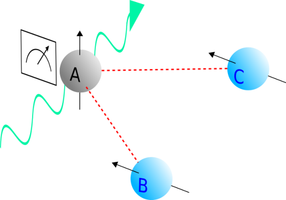
Specifically, we encode and stabilize the Bell states in a couple of mutually noninteracting qubits ( and ) by repeated projective measurements of the state of a shared ancilla qubit () which may also driven by local control fields (see Fig. 1). The sequence of measurements is performed starting with the full system in the factorized state with the three qubits in the same spin state. A readily implementable form of feedback, i.e., a ramp of the control field on triggered by a specific outcome of the measurement, ensures that in the ideal case of perfect isolation from the environment the protocol yields a Bell state with probability 1. Moreover, the sequence of outcomes of the measurements on , unambiguously identifies the specific Bell state in which the target qubits and are left asymptotically. One can then switch among the four Bell states encoded in by addressing locally either or with a single qubit operation [41], an action that does not require proximity or interaction between the entangled qubits. The feasibility of our scheme benefits from the progress in rapid high-fidelity, single-shot readout in circuit QED, superconducting qubits, and spins in solid state systems [42, 43, 44, 45, 46, 47, 48, 49, 50].
By analysing the results of the protocol with different inter-measurement times, we are able to identify the optimal rate of measurements to generate stable Bell states in a minimal amount of time. This is crucial for successfully producing a Bell state before the detrimental effects of environmental noise spoil the protocol [51]. We then use this optimal rate to examine how stable Bell states in the target qubits can be produced in a short time window, comprising measurements on ancilla , before the latter is disconnected leaving the target qubits isolated. We explicitly depict sample time evolutions of the density matrix, corresponding to different realizations of the measurement sequences.
II Setup
The model considered in our protocol consists of an open one-dimensional chain comprised of three -spins , , and (the qubits, see Fig. 1). The central spin plays the role of an ancilla and is connected to the measurement apparatus which projectively monitors its spin state in the -direction. The ancilla can be driven by a control field along the -axis. The target spins and interact exclusively with . We assume that dephasing and relaxation effects from the environment do not affect the system, at least on the time scale of the protocol with optimal monitoring rate (see below).
The inter-spin coupling and the control field are adjusted by control functions and , respectively, both assuming values in .
The Hamiltonian reads:
| (1) |
where denote the Pauli spin operators () of spin . Here the couplings and determine the magnitude of interaction and the field strength, respectively. The dynamics of the three qubit-system between consecutive measurements is induced by the Hamiltonian in Eq. (1). Thus, the time evolution of the total density matrix of the tripartite system , is governed by the Liouville-von Neumann equation
| (2) |
Throughout the present work we scale energies and times with the coupling which can be in practice very small, favoring the isolation of the target qubits, but at the expense of a longer duration of the protocol. Accordingly, we consider for the control field driving the ancilla the (maximal) value .
The state of the three qubits (ancilla and target qubits ) are expressed in the basis , where are the eigenvalues of the operators
| (3) |
with , and , respectively. We consider repeated projective measurements of which are assumed to be instantaneous, meaning that they take place on a time scale which is much smaller than the dynamical time scales of the system. Each measurement on the ancilla projects the state of the full system into one of the eigensubspaces corresponding to the eigenvalues and of .
In the next sections we study the time evolution of the system subject to repeated measurements of , starting from the fully separable initial state with set to zero. After each measurement, the density matrix evolves unitarily with respect to , until the next measurement is performed. The cycle is repeated for an overall time comprising several inter-measurement times.
III Evolution under nonselective monitoring and optimal inter-measurement time.
In our protocol, measurements of the spin state of the ancilla occur at equally-spaced times instants , where is the inter-measurement time and . The scope of the present section is to establish how the time needed to eventually reach an asymptotic state depends on . For this purpose, we study the evolution of the system undergoing a sequence of nonselective measurements in the absence of external fields, i.e., , and with . In a nonselective measurement the outcome is disregarded or simply not available, thus yielding only a probabilistic information about the post-measurement state of the system. This is in distinct contrast to the case of selective measurement where each measurement prepares the system in the eigenstate corresponding to the outcome of the measured operator. A nonselective measurement of reduces the state of the entire system to a probabilistic mixture of projections into the eigenstates and [see Eq. (3)]. This transformation is provided by the action of the projectors with . Indeed, immediately after the -th nonselective measurement, taking place at time , the density matrix of the total system can be written as
| (4) |
where is the time evolution operator from to .

In the presence of repeated nonselective measurements, the density matrix at an arbitrary time is calculated as follows. Starting at the initial time in the state , the density matrix is propagated through Eq. (2) for a time span after which the coherences between and the target qubits and are removed upon measuring the state of , according to Eq. (4). Then, the post-measurement state described by Eq. (4) is used as the initial condition for a further propagation up to time where a second measurement takes place. The above sequence is repeated and the total number of measurements occurring up to time is given by the integer part of . A scheme of this sequence is depicted in Fig. 2. We find that, for any non-pathological choice of the inter-measurement time , i.e., for inter-measurement times that do not match multiples of the free system periodicity, the asymptotic state
| (5) | |||||
is eventually reached, where the four Bell states are defined as
| (6) |
Note that the Bell state does not appear in Eq. (5). This is due to the particular initial condition chosen, as explained in Appendix A. Inspection of Eq. (5) reveals that, once the asymptotic state is attained, a further measurement on , with available outcome, yields for the target qubits and the Bell state conditioned on the readout , which occurs with probability . On the other hand, the outcome yields for the target qubits a probabilistic mixture of Bell states.
In the following section and in Appendix B,
a protocol that also yields the other entangled states and as pure states is specified.
To establish the optimal inter-measurement time for which the asymptotic state is reached in the least amount of time, we consider the trace-distance between the time-evolved density operator and the asymptotic state . This quantity is defined as
| (7) | |||||
with denoting the eigenvalues of the Hermitian matrix .
The results for the trace distance as a function of time and of the inter-measurement time are depicted in Fig. 3 for (no external field on ) and (constant qubits-ancilla coupling), see Eq. (1).

The plot in Fig. 3(a) shows that an optimal inter-measurement time around the value exists which corresponds to the minimal time needed to relax to the final state (see the horizontal dashed line). The curves depicted in Fig. 3(b) clearly show that, for , the asymptotic state is reached after few measurements whereas deviations from this optimal inter-measurement time entail a considerably larger number of measurements. Indeed, in the limit of very small – well below the optimal level – the system enters the quantum Zeno regime, as witnessed by the freezing of the trace distance from the asymptotic state at its initial value (see the lower part of Fig. 3(a)) 11 1 In a different setup [52], measurements of the joint state of two qubits are proposed to entangle the qubits by exploiting the Zeno effect occurring at large measurement rates. Here, instead, we operate in the opposite regime where measurements at an appropriate, intermediate rate produce the fastest relaxation to a target state.. On the other hand, upon increasing the inter-measurement time above the optimal value the measurements eventually synchronize with the periodicity of the free system so that oscillations persist for long evolution times around selected values of , as shown in the upper part of Fig. 3(a).
IV Selective evolution under projective measurements and feedback
Next we focus on the selective evolution of the system under the same sequence of repeated measurements on detailed in Sec. III (see Fig. 2). In this case the individual realizations of the time evolution of determined by specific sequences of random outcomes of the measurements on are considered. We show that the protocol converges to a factorized state with , with the reduced system in a Bell state.
The evolution under selective measurements is calculated as follows: Starting at with the system in the state , the full density matrix is evolved according to Eq. (2) for a time span . At time the first measurement takes place yielding a random outcome generated with probability . The state of the system is then updated to the post-measurement state which is in turn used as the initial condition for a further unitary evolution of duration and so on. The process, with the measurements taking place at times , is depicted in Fig. 2. The explicit expression for the state immediately after the -th measurement with outcome is
| (8) |
The process described yields random realizations of the time evolution of the density matrix. The expression for the probability associated to a specific realization, i.e., to a specific readout sequence , is given in Appendix B [see Eq. (28)].
In the absence of a control field (), we find two possible behaviors: Either the repeated measurements on yield an uninterrupted sequence of ’s, and the system is asymptotically left in the state , or the sequence randomly flips between the two outcomes and . In the latter case the state of the system flips between the two states and .
In Appendix B we account for this behavior by explicitly considering actual realizations of the selective evolution.

To cope with the oscillating behavior taking place in a subset of the realizations of the protocol, a simple feedback scheme can be implemented which does not require particular precision in its execution. A ramp of the control field acting on [see Eq. (1)] is turned on triggered by the first readout of a in the sequence of measurements. Specifically, the field is initially zero and is then switched on at the time when a first detection of the state of with outcome occurs during the protocol. If no outcome is found the field stays off during the evolution [see for example panel (a) of Fig. 4 below]. Let be the total duration of the protocol. The switching function is the smooth ramp
| (9) |
see Fig. 4(a)-(c).
The stabilizing effect on the oscillating sequences is due to the large value () of which makes the field term dominating with respect to the interaction term in the Hamiltonian (1). As a result, a state with a definite eigenvalue of , such as a post-measurement state, is approximately an eigenstate of the Hamiltonian and does not evolve on the time scales of the protocol. We note that this stabilizing effect – and thus the results in the present work – does not depend on the precise form of the ramp . The final part of the protocol consists in switching off the interaction strength : The interaction is held constant [] throughout the protocol and is switched off at time , i.e., , after the target qubits and have reached a steady state.
In Fig. 4, the time evolution of the reduced density matrix under selective measurements is shown for three sample realizations of the protocol. These realizations end up with the target qubits left in different Bell states, corresponding to different sequences of the measurement readouts. The readout sequences are also shown for each sample time evolution along with the behavior of the control field acting on . In the numerical simulations, the inter-measurement time is fixed at the optimal value and the switch off takes place at , namely, after measurements. A realization of the protocol leaves the target qubits in the Bell state with probability or in one of the Bells states and with total probability , (see the definitions in Eq. (6)). Although the protocol generates the Bell states non-deterministically, once the steady state is reached they are unambiguously identified by reading the sequence of outcomes of the measurements on . Having identified the Bell state encoded in the system , one can act locally on qubit or , by applying a rotation of the state of the qubit, to switch to a different Bells state [41].
A scheme of the protocol is provided in the upper panel of Fig. 5, where the three realizations in Fig (4)(a)-(c) are associated to the corresponding readout sequences and the final Bell state for the target qubits and . Note that, by using a different initial condition, the final Bell states associated to definite readout sequence can differ from the ones described here. This is exemplified in Appendix C, where the protocol is carried out with the three qubits initially prepared in the state .

To study the degree of entanglement during the protocol, we evaluate the concurrence of the reduced density matrix of the target system . This quantity is defined as , where the ’s are the ordered eigenvalues of the matrix [6, 7]. The concurrence takes values between zero and one, corresponding to non-entangled (zero) and maximally entangled states (one), respectively. The results are depicted in Fig. 4(d) for the three sample realizations displayed in panels (a)-(c). In addition, we confirm that the reduced two-qubit system is left in the specific Bell state corresponding to a particular readout sequence. This is done by calculating the fidelity [53, 54], given by the expression
| (10) |
where the referential density matrix is chosen a posteriori, as the final state that corresponds to the readout sequence (see the upper panel of Fig. 5). The time evolutions of the fidelity for the sample evolutions in Fig. 4 are depicted in the lower panel of Fig. 5.
We conclude this section by noting that, in a realistic situation, environmental effects are present, especially on the ancilla qubit which is connected to the meter. This makes the choice of the optimal time crucial in order to conclude the protocol before these detrimental effects spoil it. However, the realizations of the protocol in the classes depicted in Fig. 4(a) and (b) are expected to be more robust with respect to the environmental influence, as compared to those where the large control field acting on freezes the system in the higher energy state . In this latter case, the large energy splitting may cause the decay before the protocol is completed.
Alternatively, one may think of freezing the oscillations between and by the Zeno effect, namely by suddenly let the inter-measurement time
go to zero after a measurement on the ancilla with outcome .
V Conclusions
With this work a simple protocol is presented for generating Bell states in a couple of qubits which do not interact directly. The qubits are entangled by means of repeated projective measurements of the state of a shared ancilla qubit. We have shown that the protocol yields a definite and stable Bell state, starting from the completely factorized state of the full system. This is attained by acting on the ancilla with a suitable form of feedback, namely a ramp of a control field [see Eq.(9)], triggered by a specific readout of the ancilla state. The backaction of the repeated measurements asymptotically yields a stationary state of the form , with and , where the Bell state is unambiguously identified by reading the sequence of measurement outcomes of the ancilla.
Acknowledgments
This work is dedicated to Wolfgang P. Schleich, a great scientist and constant source of inspiration, on the occasion of his 60th birthday. P. H. and P. T. also thank Wolfgang for his vivid and illuminating many discussions and constructive debates during our yearly, alternating Augsburg-Ulm workshops. In addition P. H. likes to thank Kathy and Wolfgang for their lifetime-long wonderful friendship.
Appendix A Asymptotic state for nonselective repeated measurements with different initial conditions
To gain insight in the reasons why, with the chosen initial separable state
| (11) |
the sequence of nonselective measurement considered in Sec. III ends up with asymptotic state in Eq. (5), it is sufficient to note that the Hamiltonian (1), in the absence of control fields and with constant interaction strength, can be written as
| (12) |
The state is an eigenstate of the Hamiltonian and the only states involved that are connected by a nonzero transition amplitude are and . Thus, with the chosen initial state, the probability to get the target qubits in the Bell state is zero, as the dynamics induced by Hamiltonian (12) is confined to the subspace spanned by and the measurements on do not affect this feature. On the other hand, by starting with a different initial state, as for example , the asymptotic state reads
| (13) | |||||
[cf Eq. (5)]. A complete list of the asymptotic states attained by starting in each of the (computational) basis states is shown in Table 1.
| init. state | |
|---|---|
| Eq. (5) | |
| Eq. (13) | |
| Eq. (5) with | |
| Eq. (13) with |
To gain an intuition on how the entries in the table are obtained, let us introduce the map that propagates the density matrix for a time span and then applies a nonselective measurement on the ancilla. This map is defined by the action
| (14) | |||||
Then, the asymptotic state is given by
| (15) |
Now, let be the operation that flips the state of spin in the computational basis (the eigenbasis of ). For , both the Hamiltonian and the projectors are invariant under such operation, we have
| (16) |
and similarly and . It follows that flipping the spin of either or in the initial state returns the asymptotic state in Eq. (5) with the spin of or flipped, i.e., Eq. (13). On the other hand, flipping both the spins of and in the initial state returns the asymptotic state (5) itself, because . The above reasoning accounts for the first two rows of Table 1.
In a similar way, by writing we see that the Hamiltonian is invariant under the action of and that , which entails [see Eq. (14)]. This accounts for the last two rows of Table 1.
Appendix B Details of the selective evolution
Let us inspect the actual realizations of the time evolution given by repeatedly measuring the state of in a selective fashion, starting from the state in the absence of control fields, . The action of the time evolution operator induced by the Hamiltonian (12) for a time span is
| (17) |
with , where and depend on . The first measurement on the ancilla collapses this evolved state into one of the two alternative outcomes
| (18) |
where the indexes are used for bookkeeping the sequence of outcomes and . Then, evolving the above states for another time span we get
| (19) | |||||
| (20) |
Upon measuring again the state of the following two couples of alternative outcomes arise
and so on. From this behavior it is clear that, for , i.e., if is not a multiple of the period of the unitary evolution, a long sequence of outcomes will yield the stabilized state , meaning that a further measurement will leave the system in this same state with probability . On the other hand, the presence of zeroes in the readout sequences entails oscillations between and which last indefinitely. This behavior is very close to what is found in Ref [55] by simulating the repeated parity measurements in a couple of double quantum dot qubits. The probability associated to a specific sequence of outcomes , where , is given by
| (27) |
where, as in Eq. (4), is the time evolution operator from to . By extrapolating from the sequence in Eqs. (17)-(B) one sees that the probability to obtain an interrupted sequence of readouts is
| (28) |
Appendix C Realizations of the protocol with a different initial condition

References
- [1] W. P. Schleich 2001 Quantum Optics in Phase Space (Wiley-VCH, Berlin).
- [2] J. L. O’Brien, A. Furusawa, and J. Vučković. Photonic quantum technologies. Nat. Photonics, 3:687 EP–, 12 2009.
- [3] R. Horodecki, P. Horodecki, M. Horodecki, and K. Horodecki. Quantum entanglement. Rev. Mod. Phys., 81:865–942, Jun 2009.
- [4] V. Giovannetti, S. Lloyd, and L. Maccone. Advances in quantum metrology. Nat. Photonics, 5:222 EP, 03 2011.
- [5] G. Tóth and I. Apellaniz. Quantum metrology from a quantum information science perspective. J. Phys. A, 47(42):424006, 2014.
- [6] S. Hill and W. K. Wootters. Entanglement of a Pair of Quantum Bits. Phys. Rev. Lett., 78:5022–5025, Jun 1997.
- [7] W. K. Wootters. Entanglement of Formation of an Arbitrary State of Two Qubits. Phys. Rev. Lett., 80:2245–2248, Mar 1998.
- [8] J. P. Dahl, H. Mack, A. Wolf, and W. P. Schleich Entanglement versus negative domains of Wigner functions Phys. Rev. A, 74(4), 042323, Oct 2006.
- [9] M. Steffen, M. Ansmann, R. C. Bialczak, N. Katz, E. Lucero, R. McDermott, M. Neeley, E. M. Weig, A. N. Cleland, and J. M. Martinis. Measurement of the Entanglement of Two Superconducting Qubits via State Tomography. Science, 313(5792):1423–1425, 2006.
- [10] F. Galve, D. Zueco, S. Kohler, E. Lutz, and P. Hänggi. Entanglement resonance in driven spin chains. Phys. Rev. A, 79:032332, Mar 2009.
- [11] F. Galve, D. Zueco, G. M. Reuther, S. Kohler, and P. Hänggi. Creation and manipulation of entanglement in spin chains far from equilibrium. Eur. Phys. J. Special Topics, 180(1):237–246, 2009.
- [12] R. Blattmann, H. J. Krenner, S. Kohler, and P. Hänggi. Entanglement creation in a quantum-dot-nanocavity system by Fourier-synthesized acoustic pulses. Phys. Rev. A, 89:012327, Jan 2014.
- [13] M. B. Plenio and S. F. Huelga. Entangled Light from White Noise. Phys. Rev. Lett., 88:197901, Apr 2002.
- [14] F. Verstraete, M. M. Wolf, and J. I. Cirac. Quantum computation and quantum-state engineering driven by dissipation. Nat. Phys., 5:633 EP, 07 2009.
- [15] D. Zueco, G. M. Reuther, P. Hänggi, and S. Kohler. Entanglement and disentanglement in circuit QED architectures. Physica E, 42(3):363–368, 2010.
- [16] P.-B. Li, S.-Y. Gao, H.-R. Li, S.-L. Ma, and F.-L. Li. Dissipative preparation of entangled states between two spatially separated nitrogen-vacancy centers. Phys. Rev. A, 85:042306, Apr 2012.
- [17] Z. Leghtas, U. Vool, S. Shankar, M. Hatridge, S. M. Girvin, M. H. Devoret, and M. Mirrahimi. Stabilizing a Bell state of two superconducting qubits by dissipation engineering. Phys. Rev. A, 88:023849, Aug 2013.
- [18] M. E. Kimchi-Schwartz, L. Martin, E. Flurin, C. Aron, M. Kulkarni, H. E. Tureci, and I. Siddiqi. Stabilizing Entanglement via Symmetry-Selective Bath Engineering in Superconducting Qubits. Phys. Rev. Lett., 116:240503, Jun 2016.
- [19] M. Benito, M. J. A. Schuetz, J. I. Cirac, G. Platero, and G. Giedke. Dissipative long-range entanglement generation between electronic spins. Phys. Rev. B, 94:115404, Sep 2016.
- [20] F. Reiter, D. Reeb, and A. S. Sørensen. Scalable Dissipative Preparation of Many-Body Entanglement. Phys. Rev. Lett., 117:040501, Jul 2016.
- [21] X.-X. Li, P.-B. Li, S.-L. Ma, and F.-L. Li. Preparing entangled states between two NV centers via the damping of nanomechanical resonators. Sci. Rep., 7(1):14116, 2017.
- [22] D. X. Li, X. Q. Shao, and X. X. Yi. Entangled-state preparation by dissipation, dispersive coupling, and quantum Zeno dynamics. arXiv:1705.06471, 2017.
- [23] C. W. J. Beenakker, D. P. DiVincenzo, C. Emary, and M. Kindermann. Charge Detection Enables Free-Electron Quantum Computation. Phys. Rev. Lett., 93(2):020501, Jul 2004.
- [24] H.-A. Engel and D. Loss. Fermionic Bell-State Analyzer for Spin Qubits. Science, 309(5734):586, Jul 2005.
- [25] R. Ruskov and A. N. Korotkov. Entanglement of solid-state qubits by measurement. Phys. Rev. B, 67:241305, Jun 2003.
- [26] A. Kolli, B. W. Lovett, S. C. Benjamin, and T. M. Stace. All-Optical Measurement-Based Quantum-Information Processing in Quantum Dots. Phys. Rev. Lett., 97(25):250504, Dec 2006.
- [27] C. Hill and J. Ralph. Weak measurement and control of entanglement generation. Phys. Rev. A, 77:014305, Jan 2008.
- [28] N. S. Williams and A. N. Jordan. Entanglement genesis under continuous parity measurement. Phys. Rev. A, 78:062322, Dec 2008.
- [29] W. Pfaff, T. H. Taminiau, L. Robledo, H. Bernien, M. Markham, D. J. Twitchen, and R. Hanson. Demonstration of entanglement-by-measurement of solid-state qubits. Nat. Phys., 9:29 EP, 10 2012.
- [30] O.-P. Saira, J. P. Groen, J. Cramer, M. Meretska, G. de Lange, and L. DiCarlo. Entanglement Genesis by Ancilla-Based Parity Measurement in 2D Circuit QED. Phys. Rev. Lett., 112:070502, Feb 2014.
- [31] N. Roch, M. E. Schwartz, F. Motzoi, C. Macklin, R. Vijay, A. W. Eddins, A. N. Korotkov, K. B. Whaley, M. Sarovar, and I. Siddiqi. Observation of Measurement-Induced Entanglement and Quantum Trajectories of Remote Superconducting Qubits. Phys. Rev. Lett., 112(17):170501, Apr 2014.
- [32] A. Chantasri, M. E. Kimchi-Schwartz, N. Roch, I. Siddiqi, and A. N. Jordan. Quantum Trajectories and Their Statistics for Remotely Entangled Quantum Bits. Phys. Rev. X, 6(4):041052, Dec 2016.
- [33] L. Martin, M. Sayrafi, and K. B. Whaley. What is the optimal way to prepare a Bell state using measurement and feedback? Quantum Sci. Technol., 2(4):044006, 2017.
- [34] D. Ristè, M. Dukalski, C. A. Watson, G. de Lange, M. J. Tiggelman, Ya. M. Blanter, K. W. Lehnert, R. N. Schouten, and L. DiCarlo. Deterministic entanglement of superconducting qubits by parity measurement and feedback. Nature, 502:350 EP, 10 2013.
- [35] C. Meyer zu Rheda, G. Haack, and A. Romito. On-demand maximally entangled states with a parity meter and continuous feedback. Phys. Rev. B, 90:155438, Oct 2014.
- [36] E. Knill, R. Laflamme, and G. J. Milburn. A scheme for efficient quantum computation with linear optics. Nature, 409:46, Jan 2001.
- [37] D. Layden, E. Martín-Martínez, and A. Kempf. Universal scheme for indirect quantum control. Phys. Rev. A, 93(4):040301, Apr 2016.
- [38] H. Nakazato, M. Unoki, and K. Yuasa. Preparation and entanglement purification of qubits through Zeno-like measurements Phys. Rev. A, 70:012303, Jul 2004.
- [39] L.-A. Wu, D. A. Lidar, and S. Schneider. Long-range entanglement generation via frequent measurements Phys. Rev. A, 70:032322, Sep 2004.
- [40] G. Compagno, A. Messina, H. Nakazato, A. Napoli, M. Unoki, and K. Yuasa. Distillation of entanglement between distant systems by repeated measurements on an entanglement mediator Phys. Rev. A, 70:052316, Nov 2004.
- [41] J. Preskill. Lecture Notes on Quantum Computation. http://www.theory.caltech.edu/people/preskill/ph229/
- [42] F. Mallet, F. R. Ong, A. Palacios-Laloy, F. Nguyen, P. Bertet, D. Vion, and D. Esteve. Single-shot qubit readout in circuit quantum electrodynamics. Nat. Phys., 5:791, 09 2009.
- [43] A. Morello, J. J. Pla, F. A. Zwanenburg, K. W. Chan, K. Y. Tan, H. Huebl, M. Möttönen, C. D. Nugroho, C. Yang, J. A. van Donkelaar, A. D. C. Alves, D. N. Jamieson, C. C. Escott, L. C. L. Hollenberg, R. G. Clark, and A. S. Dzurak. Single-shot readout of an electron spin in silicon. Nature, 467:687 EP, 09 2010.
- [44] P. Neumann, J. Beck, M. Steiner, F. Rempp, H. Fedder, P. R. Hemmer, J. Wrachtrup, and F. Jelezko. Single-Shot Readout of a Single Nuclear Spin. Science, 329(5991):542, 07 2010.
- [45] L. Robledo, L. Childress, H. Bernien, B. Hensen, P. F. A. Alkemade, and R. Hanson. High-fidelity projective read-out of a solid-state spin quantum register. Nature, 477:574 EP, 09 2011.
- [46] J. J. Pla, K. Y. Tan, J. P. Dehollain, W. H. Lim, J. J. L. Morton, F. A. Zwanenburg, D. N. Jamieson, A. S. Dzurak, and A. Morello. High-fidelity readout and control of a nuclear spin qubit in silicon. Nature, 496:334 EP, 04 2013.
- [47] A. Delteil, W. Gao, P. Fallahi, J. Miguel-Sanchez, and A. Imamoǧlu. Observation of Quantum Jumps of a Single Quantum Dot Spin Using Submicrosecond Single-Shot Optical Readout. Phys. Rev. Lett., 112(11):116802, 03 2014.
- [48] P. Krantz, A. Bengtsson, M. Simoen, S. Gustavsson, V. Shumeiko, W. D. Oliver, C. M. Wilson, P. Delsing, and J. Bylander. Single-shot read-out of a superconducting qubit using a Josephson parametric oscillator. Nat. Comm., 7:11417, 2016.
- [49] T. Walter, P. Kurpiers, S. Gasparinetti, P. Magnard, A. Potočnik, Y. Salathé, M. Pechal, M. Mondal, M. Oppliger, C. Eichler, and A. Wallraff. Rapid High-Fidelity Single-Shot Dispersive Readout of Superconducting Qubits. Phys. Rev. Applied, 7:054020, May 2017.
- [50] D. M. Zajac, A. J. Sigillito, M. Russ, F. Borjans, J. M. Taylor, G. Burkard, and J. R. Petta. Resonantly driven CNOT gate for electron spins. Science, Dec 2017.
- [51] J. D. Wong-Campos, S. A. Moses, K. G. Johnson, and C. Monroe. Demonstration of Two-Atom Entanglement with Ultrafast Optical Pulses. Phys. Rev. Lett., 119(23):230501, Dec 2017.
- [52] X.-B. Wang, J. Q. You, and F. Nori. Quantum entanglement via two-qubit quantum Zeno dynamics. Phys. Rev. A, 77(6):062339, Jun 2008.
- [53] A. Uhlmann. The “transition probability” in the space of a ∗-algebra. Rep. Math. Phys., 9(2):273–279, Oct 1976.
- [54] R. Jozsa. Fidelity for Mixed Quantum States. J. Mod. Opt., 41(12):2315–2323, 12 1994.
- [55] B. Trauzettel, A. N. Jordan, C. W. J. Beenakker, and M. Büttiker. Parity meter for charge qubits: An efficient quantum entangler. Phys. Rev. B, 73:235331, Jun 2006.