The P2 Experiment
Abstract
This article describes the research and development work for
the future P2 experimental facility at the upcoming MESA
accelerator in Mainz. The facility is optimized for the detection
of order parity-violating cross section asymmetries in
electron scattering. The physics program of the facility comprises
indirect, high precision search for physics beyond the Standard
Model, measurement of the neutron distribution in nuclear physics,
single-spin asymmetries stemming from two-photon exchange and a
possible future extension to the measurement of hadronic parity
violation.
The first measurement of the P2 experiment for which the research
and development work is most advanced is described here in detail.
It aims for a high precision determination of the weak mixing
angle to a precision of at a four-momentum
transfer of GeV2. The accuracy is
comparable to existing measurements at the pole.
It comprises a sensitive test of the standard model up to a mass
scale of , extendable to .
This requires a measurement of the parity violating cross section
asymmetry
in the elastic electron-proton scattering with a total accuracy
of (1.4%) in of polarized
electron beam impinging on a target
allowing for an extraction of the weak charge of the proton
which is directly connected to the weak mixing angle .
Contributions from -box graphs become small at the
small beam energy of .
The P2 asymmetry is smaller than any asymmetry measured so far
in electron scattering with an unprecedented goal for the accuracy.
The use of a solenoid-spectrometer with
-acceptance as well as an atomic H trap polarimeter are
some new features, which have never before been used in
parity-violation experiments, and which we describe among
others, here. In order to collect the enormous statistics
required for this measurement, the new Mainz Energy Recovery
Superconducting Accelerator (MESA) is under construction. The
plans on the associated beam control system and the polarimetry
is described in this article as well. A new high-power
target design with an enormously low noise level of
needs to be constructed. We report here in addition on the
conceptual design of the P2 spectrometer, its Cherenkov detectors,
the integrating read-out electronics as well as the ultra-thin, fast tracking detectors.
There has been substantial theory work done
in preparation of the determination of . The further physics
program in particle and nuclear physics is described here as well.
pacs
11.30.ErCharge conjugation, parity, time reversal, and other discrete symmetries and 12.15.LkElectroweak radiative corrections and 13.85.DzElastic scattering and 13.88.+ePolarization in interactions and scattering and 25.30.BfElastic electron scattering and 29.20.EjLinear accelerators and 29.27.HjPolarized beams and 29.40.GxTracking and position-sensitive detectors and 29.40.KaCherenkov detectors1 Introduction and physics motivation
In the Standard Model of Elementary Particle Physics (SM) the weak interaction is the only force that violates parity. Over the past 30 years, the measurement of parity violation in weak interactions has been a well established experimental technique in atomic as well as particle and nuclear physics. The violation of parity had been postulated by the theoreticians Lee & Yang in 1956 [1]. It was proven to be an experimental fact in nuclear physics in in the course of the Wu experiment [2] by a careful analysis of the beta-decay of . In addition Garwin, Lederman and Weinrich had shown that the -decay violates parity [3]. As first pointed out by Zeldovich in 1959 [4], the existence of a neutral partner of the charged weak interaction responsible for -decay, should lead to observable parity violation in atomic physics and in electron scattering. These ideas preceded the development of the electroweak theory, and were confirmed experimentally by Prescott in electron scattering at SLAC [5] and in cesium atoms by Bouchiat [6]. In the rest of this article we concentrate on parity violation in electron scattering.
Since then, many parity-violating electron scattering experiments have been performed, all summarized in Fig. 1. Prescott’s experiment was followed by an experiment of the Mainz group of Otten and Heil [7] and another one at MIT-Bates on a 12C target [8]. Their experimental techniques were pioneering and are used still today. They were also ground-breaking in establishing parity-violation and making the first measurements of SM parameters from electron scattering (see the green points in Fig. 1 labeled “Pioneering”).
It was first pointed out by Kaplan and Manohar in 1988 [9] that one can get access to a possible contribution of strange quarks to the electromagnetic form factors of the nucleon by measuring its weak electric and magnetic form factors in parity-violating electron scattering. This triggered a whole series of parity-violation electron scattering experiments at the MIT-Bates accelerator [10, 11, 12, 13, 14, 15], at the MAMI accelerator in Mainz [16, 17, 18, 19, 20, 21, 22, 23, 24, 25, 26] as well as at JLab’s CEBAF in Newport News [27, 28, 29, 30, 31, 32, 33, 34, 35, 36, 37, 38, 39, 40] (see in addition [41, 42, 43, 44, 45] for review articles, blue points in Fig. 1 labeled “Strange Quark Studies”). An accurate measurement of the neutron distribution in heavier nuclei and especially the so called “neutron skin” can be obtained from parity-violating electron scattering on heavy nuclei like lead [46, 47]. The associated parity-violation experiments are labeled “Neutron Radius” in Fig. 1. In recent years, experiments have been performed and new proposals have been worked out to measure the weak charge of the proton or of the electron, or the ratio of quark charges. Those are labeled “Standard Model Tests” in Fig. 1 [48, 49, 50, 51, 52]. The parity-violating electron scattering experiments at the new Mainz MESA accelerator [53] are the subject of this manuscript.
In the P2 experiment, parity-violation in elastic electron-proton scattering at low momentum transfer, , will provide experimental access to the proton’s weak charge , the analog of the electric charge which determines the strength of the neutral-current weak interaction. In the SM, is related to the electroweak mixing angle, . The weak charge of the proton is particularly interesting, compared to that of other nuclei, since it is suppressed in the SM and therefore sensitive to hypothetical new physics effects. The SM also provides a firm prediction for the energy-scale dependence of the running of . This scale dependence, defined in the scheme, is shown in Fig. 2 together with the anticipated sensitivity of the measurement of the weak mixing angle at P2 compared to other forthcoming determinations (blue points) and existing measurements (red points).
A precise measurement of the weak charge provides, therefore, a precision test of the SM and its predictions. The envisaged measurement of the P2 experiment at low momentum transfer will complement other high-precision determinations, like those of the LEP and SLC experiments at the pole. The P2 experiment may thus help to resolve differences between previous measurements, or find interesting new effects.
Extensions of the SM lead to modified predictions for various observables, visible only in high-precision measurements. For example, models with dark photons predict a small shift of the running weak mixing angle at low mass scales, i.e., a change of visible at P2, but not at the -pole measurements. Other models, like supersymmetry, lead to characteristic deviations for different observables and only a combined analysis can reveal the type of new physics. A convenient way to compare the reach of different observables to the mass scale, , of new physics is based on a description with effective 4-fermion operators. Following the convention that the relevant coupling constant is normalized by , one can estimate the reach by where is the Fermi constant and the precision for the measurement of the weak charge. At P2, the measurement of the weak charge of the proton is expected to reach mass scales close to [55]. Other targets, like 12C may increase this limit even further.
Our understanding of the electroweak interactions will improve
considerably by the forthcoming high-precision experiments.
The measurement of the weak charge is expected to improve by
a factor of 3 compared to the anticipated precision achieved
by the QWeak collaboration at JLab [54].
Similarly, the MOLLER experiment at JLab
will provide us with a factor of 5 improvement of the
determination of the weak charge of the electron, compared
with the result of the E158 experiment at SLAC. Also the
ratio of - and -quark weak charges will be measured
more precisely than before at the SOLID experiment at JLab.
If completed, the combination of these experiments will
offer us a handle to distinguish extensions of the SM, which
contribute in different ways to these experiments.
The Mainz MESA electron accelerator with the P2 experimental facility for parity-violation experiments opens a door to a rich parity-violation measurement program including different targets and kinematics. This is partly described in the Sect. 7. This research program has its roots in discussions at a workshop at MIT, organised by MIT, JLab, and Mainz in 2013. For more information, see [53].
The second experimental facility at MESA is MAGIX. It will be
equipped with two magnetic spectrometers and a hydrogen cluster
jet target. MAGIX has a rich program in nucleon and nuclear
physics, including measurements of the proton radius, the
electromagnetic form factors of the nucleon, measurements of
nuclear cross sections relevant for open questions in astrophysics,
and dark photon searches in scattering and in a beam dump experiment.
Also the MAGIX research program was discussed at the
aforementioned MIT workshop.
This manuscript is organized as follows: In Section 2 we describe how – and how accurate – we can extract the weak mixing angle from the measurement of the parity-violating cross section asymmetry. In Section 3 we describe the new MESA accelerator which will be installed in a new accelerator hall from 2020 on. This Section also describes the polarimetry at MESA as well as the control of helicity-correlated and uncorrelated beam fluctuations. For the measurement proposed here, a liquid hydrogen target with the lowest possible level of density fluctuations ( in ) from boiling in the volume of the H2 or from other sources will represent one of the centerpieces. The design approach, the method to calculate the density fluctuations beforehand and the experience from the design of the H2 target at the former QWeak experiment are described in Sect. 4. The P2 spectrometer, consisting of the H2 target, the large solenoid magnet, the results of the full Geant4 simulations of the spectrometer, the integrating Cherenkov detectors, the high-resolution ADC system for the read-out as well as the tracking detector is presented in Sect. 5. The new level of experimental accuracy required in the past, and still requires, corresponding theory efforts in order to get effects from QED corrections, box graph and hadronic uncertainties and other electroweak radiative corrections under control. The relevant recent theory work is described in Sect. 6. The P2 experimental facility for parity-violating electron scattering allows for a rich measurement program, like an additional backward-angle measurement to further reduce the uncertainty from the axial form factor and the contribution from strangeness to the magnetic form factor. Both are not sizeable quantities, but still have large error bars. Another example is an additional measurement with a 12C target. This allows for an even more sensitive search for beyond Standard Model physics. A very sensitive measurement of the neutron skin thickness in lead is possible with the P2 spectrometer as well. This exciting further physics program at the P2 experimental facility is described in Sect. 7. The manuscript presented here closes with a summary.
2 Determining the Weak Mixing Angle from Parity Violating Electron Scattering
In this chapter, the experimental method for measuring the proton’s weak charge is presented and the achievable precision in the determination of the electroweak mixing angle is discussed.
2.1 Experimental method
For the P2 experiment, MESA will provide a beam of longitudinally polarized electrons. The beam energy will be
| (1) |
and the beam current is scheduled to be
| (2) |
The helicity of the beam electrons will be switched with a frequency . The beam electrons impinge on an unpolarized -target with a length of oriented along the beam direction. The electrons, which are scattered elastically off the protons, are detected in an azimuthally symmetric Cherenkov detector. Figure 3 illustrates the measurement principle.
Since the luminosity of the P2 experiment is projected to be
| (3) |
where is the elementary charge and is the proton density in , the total rate of the electrons scattered elastically off protons which needs to be detected is in the order of . This makes an integrating measurement of the event rates necessary.
2.1.1 Parity-violating asymmetry in elastic electron-proton scattering
The main observable in the P2 experiment is the parity-violating asymmetry in elastic electron-proton scattering. It is an asymmetry in the cross section which may be defined by
| (4) |
In this equation, is the differential cross section for the elastic scattering of electrons with helicity off unpolarized protons.
is due to the interference between the exchange of a virtual photon and a -boson in the scattering process, both of which are illustrated in Fig. 4. The differential cross section of the scattering process can be written
| (5) |
where is the electromagnetic coupling, is the proton mass, and
| (6) |
is the negative square of the 4-momentum transfer between electron and proton. Here, the electron mass can be neglected. is the electron’s initial state energy, the energy of the scattered electron and the scattering angle with respect to the beam direction. is the transition matrix element, at leading order given by the Feynman diagrams shown in Fig. 4.
The resulting parity-violating helicity asymmetry is written as
| (7) |
where is the Fermi coupling constant. Here, the weak charge of the proton, , is defined as the limit of the asymmetry at zero-momentum transfer, normalized such that Eq. (7) holds, i.e., . At non-zero momentum transfer, the hadronic structure of the proton has to be taken into account, parametrized by the - and energy-dependent function . The function is often written as and the energy-dependence not shown explicitly.
Based on a flavour decomposition of the matrix elements of the electromagnetic and weak neutral currents, the form factor contribution is usually written as a sum of three terms
| (8) |
where
| (9) |
is given by the proton’s electric and magnetic form factors and as well as the neutron’s electric and magnetic form factors and . depends on the proton’s axial form factor and is denoted as
| (10) |
depends on the nucleon’s strange electric and magnetic form factors and as well as the isospin-breaking form factors and :
| (11) |
In these expressions we have used the abbreviations
| (12) |
and
| (13) |
According to Eq. (7), is proportional to . In Fig. 5 we show the dependence of on for , which equals the beam energy to be used in the P2 experiment. The picture also shows the separate contributions
| (14) |
to . One can see that at low , is dominated by , while the hadronic contributions are small. A measurement of at low is therefore sensitive to the weak charge of the proton, .
2.1.2 The proton’s weak charge and the electroweak mixing angle
Neglecting radiative corrections, the tree-level expression for the proton’s weak charge in (7) is
| (15) |
where is the electroweak mixing angle or Weinberg-angle. In the following we will often use the abbreviation . Since , is small in the SM. From (15), using Gaussian error propagation, it follows that
| (16) |
Therefore, a precise measurement of will result in an approximately times more precise determination of the electroweak mixing angle. The weak charge of the proton is therefore highly sensitive to the electroweak mixing angle.
Even small corrections to may modify significantly. A wide range of beyond-SM effects can lead to such corrections. They need to be disentangled from SM radiative corrections. Higher-order corrections to will be discussed later in Sect. 6.
2.2 Achievable precision in the determination of the weak mixing angle
In order to predict the achievable precision in the determination of , error propagation calculations based on the Monte Carlo method have been carried out. The goal of these calculations was to determine the achievable uncertainty as a function of the beam energy , the central electron scattering angle and the acceptance of the azimuthally symmetric detector in , denoted . In the following, the method used to calculate will be discussed and results of the calculations will be presented. Based on these results, the beam energy and detector acceptance to be used in the P2 experiment are chosen.
2.2.1 Method to determine the achievable uncertainty of
The analysis presented in this section is based on the leading-order prediction of . Therefore we use the generic symbol for the sine of the weak mixing angle. Only if higher-order corrections are included, one will have to distinguish between the on-shell or the definitions of and, in the latter case, specify its scale-dependence.
In a parity-violation electron scattering experiment, one measures the asymmetry
| (17) |
which is determined by the total numbers of detected scattering events for the two helicity states of the beam electrons. One can write
| (18) |
where is the average polarization of the electron beam,
| (19) |
is the expected value of after averaging over the target length and the detector acceptance in . In addition, the polarization independent part of the differential cross section
| (20) |
given by the Rosenbluth formula [56] is taken into account. Furthermore, is an apparative asymmetry induced by helicity-correlated fluctuations of the electron beam’s properties. In Eq. (19), the averaging over the target’s length is done to include the mean energy loss of the beam electrons due to collision and radiation processes as they travel through the target volume. At leading-order, both and may be regarded as functions of the electron’s mean initial state energy and scattering angle . depends on the -coordinate of the interaction vertex’s position in the target and decreases with increasing penetration depth of the beam electrons.
To predict , Eq. (18) is solved for , and an error propagation calculation based on the resulting expression is performed. This expression has the general structure
| (21) | |||||
where represents parametrizations of the nucleon’s form factors which depend on a set of independent, real parameters , and are the contributions from -box graphs. Therefore, one may consider a function of a set of independent parameters :
| (22) |
with
| (23) |
The Gaussian error propagation based on Eq. (22) is not straightforward, since the integrations in Eq. (19) cannot be done analytically.
Therefore, Monte Carlo based error propagation calculations have been carried out numerically. The idea is to treat the parameters as independent random variables and to calculate a distribution of values by inserting the randomized parameters into Eq. (22). The first step to achieve this is to assign a Gaussian probability distribution to each parameter by defining the distribution’s mean value and standard deviation . One then samples a set of random values according to the assigned probability distributions using a random number generator. Substituting the randomized values into Eq. (22) leads to
| (24) |
Iterating this procedure leads to a distribution of values, from which the expected value and standard deviation can be extracted. While the mean value is expected to match the input value of used to calculate , is in the following regarded as the achievable precision in the determination of the electroweak mixing angle.
The algorithm allows to calculate the contributions of individual parameters to by sampling only the parameter whose contribution is of interest while all other parameters are kept constant at their expected values. Furthermore, it is possible to compute the expected value and the uncertainty of by sampling a distribution of -values. This distribution is generated by repeatedly calculating values of for the same choice of and . From the resulting distribution of values, both the mean value and the standard deviation are extracted.
2.2.2 Input parameters to the calculation of
The mean values and standard deviations of the parameters are chosen according to the projected experimental conditions of the experiment. Table 1 lists all parameter values related to the experimental conditions at the MESA facility. A systematic scan of the mean values of has been performed in order to determine appropriate values for these parameters for the design of the experimental apparatus.
| variable | ||
| variable | ||
| variable | ||
The expected value of the asymmetry is calculated by inserting the mean values of the relevant parameters into Eq. (18). As standard deviation the statistical uncertainty of is chosen. Assuming Poisson-statistics and starting from Eq. (18), one finds that
| (25) |
where it has been assumed that
| (26) |
In addition to the uncertainty contributions to originating from the experiment-related parameters listed in Tab. 1, one expects a significant contribution from the -box graph. At , one expects
| (27) | |||||
| (28) |
for the central value and the uncertainty of [57]. Details of the box-graph corrections and the definition of are discussed in Sect. 6.1.
It has been assumed in Eq. (21) that the nucleon form factors can be parametrized as functions , where is a set of independent, real parameters. In the following, we present the parametrizations of the nucleon form factors that have been used to carry out the error propagation calculations.
Electromagnetic form factors of the proton.
The form factors and have been parametrized using the “Dipole Polynomial-Model”, which has been developed by Bernauer et al. [58]. In this model, the standard dipole term
| (29) |
is multiplied by a polynomial
| (30) |
such that
| (31) |
where is the proton’s magnetic moment and is the nuclear magneton. In order to retrieve the parameters of the parametrization, Eq. (31) has been fitted to the data sets given in section K 2.2.3 of [58], leading to the parameter values listed in the Appendix, Tabs. 17 and 18.
Electromagnetic form factors of the neutron.
The functions used to parametrize and have been chosen as in Ref. [59]. For , a fit function according to Galster [60] has been used:
| (32) |
where is defined in Eq. (31) and in Eq. (13). The fit of Eq. (32) to the data set given in [59] leads to the parameter values listed in Tab. 19. In order to parametrize the neutron’s magnetic form factor a polynomial of degree is used:
| (33) |
Fitting Eq. (33) to the data given in [59] results in the parameters listed in Tab. 20.
Strangeness form factors.
The experimental determination of the strangeness form factors and has been the subject of a comprehensive measurement program for years in three major research facilities. Measurements with , and have been carried out by the SAMPLE, HAPPEX, G0 and the A4 Collaborations [14, 35, 33, 37, 16, 24].
Like , has been parametrized using Eq. (32). Fitting this expression to the available world data leads to the parameter values presented in Tab. 21. For , the parametrization
| (34) |
which was taken from Ref. [61], has been used along with the parameter values given in Tab. 22.
In the following it is assumed that the uncertainties of and can be reduced by factors of and , respectively, in the region of relevance to the P2 experiment. This reduction can be achieved by an additional backward-angle measurement, see Sect. 7.3.
Axial form factor of the proton.
The axial form factor of the proton can be determined from results of parity-violation electron scattering experiments with - and -targets, which have been carried out at backward scattering angles at the same values of . Appropriate measurements have been done by the SAMPLE, G0 and A4 Collaborations [15, 35, 37, 25].
For the purpose of the error propagation calculations presented in this section, has been parametrized as suggested by Musolf et al. in Ref. [41]:
| (35) |
This parametrization is used together with the parameter values given in [41] and listed in Tab. 23.
For the error propagation calculations presented in this section it has been assumed that the global uncertainty of the parametrization given by Eq. (35) can be reduced by a factor of . This reduction can be achieved by a backward-angle measurement of (see Sect. 7.3).
The requirement of reducing the uncertainties of , and in order to achieve the envisaged precision in the determination of renders the form factor measurement within the scope of the P2 experiment mandatory.
Isospin breaking electromagnetic form factors.
The parametrizations of the isospin-breaking form factors and have been done using the dataset quoted in the bachelor thesis of P. Larin [62]. Larin has extracted data from the predictions for the -dependence of the form factors given in [63]. In order to parametrize and , polynomials of degree have been used such that
| (36) |
The fits of these functions to the data given in Ref. [62] result in the parameter values collected in Tabs. 24 and 25.
2.2.3 Results of the error propagation calculations
An extensive scan in the mean values of , and has been performed using the input parameters discussed in the preceding section in order to determine suitable values of these variables to carry out the P2 experiment. In this section, selected results are presented and discussed.
Figure 6 shows the dependence of on the central electron scattering angle for and . For , the total uncertainty is dominated by the statistical uncertainty of the measured asymmetry . For scattering angles the contributions from and become more significant, because the form factors’ contribution to the asymmetry increases with . The increase of the form factor contributions and the decrease of the statistical error and the contribution stemming from with increasing lead to a minimum of at , where .
Figure 7 shows the dependence of on for and different choices of . In general, a larger value of leads to a larger and therefore to a smaller statistical uncertainty of . Since the statistical uncertainty of is the dominant contribution to , the achievable uncertainty in the electroweak mixing angle decreases with rising . The larger the acceptance, the smaller is the effect of increasing on , because contributions by the nucleon form factors become more significant at larger scattering angles. To keep the nucleon form factors’ contributions reasonably small, we have decided to use .
Figure 8 shows the dependence of on and for . Values of can be achieved in the region marked by a black curve.
To carry out the P2 experiment within the envisaged measurement time of , we have decided to use a beam energy of , a central scattering angle of and a detector acceptance . Table 2 lists the results of an error propagation calculation for this choice of kinematic parameters along with the error contributions stemming from the statistical uncertainty of , the contribution of the beam polarization as well as the contribution from helicity correlated beam fluctuations. In order to extract the electroweak mixing angle from the measured uncertainty, one has to take the nucleon form factors and radiative corrections to the proton’s weak charge into account. The expected contributions to due to uncertainties of the form factors and of are also listed in Tab. 2.
| () | |
| () | |
| () | |
| () | |
| () | |
| () | |
| () | |
| () | |
| () | |
| () | |
The expected value of the parity-violating asymmetry is
| (37) |
with an uncertainty of
| (38) |
in of measurement time. This corresponds to a relative uncertainty of
| (39) |
The expected uncertainty for the weak mixing angle is
| (40) |
corresponding to a relative uncertainty of
| (41) |
for and
| (42) |
for the proton’s weak charge.
2.2.4 Scattering off the target entry and exit windows
Beam electrons which scatter off the windows of the target cell are an additional source of uncertainty. This effect is briefly discussed here and will be included in the error propagation calculation (see Sect. 2.2.3).
Omitting all other sources of background and beam polarization, the measured asymmetry consists of two contributions:
| (43) |
where is the parity-violating asymmetry in eAl scattering and is the dilution factor
| (44) |
and is the yield of scattering events off aluminum and of elastic scattering off the proton, respectively. This equation can be solved for . Gaussian error propagation yields
| (45) |
Both the asymmetry of the aluminum scattering and the dilution factor need to be measured in the P2 experiment. For an estimation of the size of the effect we use measurements performed by the A4 experiment [16] and the QWeak experiment [64]. From the A4 measurements with an aluminum target which where performed at the same central scattering angle that is foreseen for P2, , but with higher electron energies from up to , we find a dilution factor of for a P2 target with a liquid hydrogen volume along the beam axis and a total thickness of for the aluminum entry and exit windows. Other window thicknesses can be calculated by simply applying the factor to this dilution factor. We plan to determine this dilution factor by measuring the detector yield with an empty target cell with an uncertainty of . The QWeak measurements with an aluminum target show that the asymmetry is about one order of magnitude larger than the asymmetry . We use this result to estimate in our case. We plan to perform a measurement with a thick aluminum target. Based on our rate estimation, the expected uncertainty of this measurement is .
Based on these numbers we can perform the error calculation. Figure 9 shows the contribution from the target window scattering to the uncertainty of as a function of the total thickness of the target windows. For example, with a total thickness of we obtain an error contribution of . It is of similar size as the error from the electron beam polarization and well below the anticipated statistical uncertainty.
3 The MESA Accelerator
The increased demand for experiments at the MESA accelerator has necessitated a new experimental hall which is currently being erected. The civil construction work will be finalized in 2020. Figure 10 shows the MESA accelerator layout with several components that are especially relevant for the P2 experiment. In P2, the beam will be extracted from the accelerator, directed towards the experiment and will be stopped afterwards in the heavily shielded beam dump building. The beam energy gain per pass is given by the acceleration capacity of the two cryomodules which are designed for each. After three passages through the cryomodules the beam energy at P2 reaches , ( per pass + from injector), lower energies are possible.

An spin-polarized beam of intensity is generated in a polarized source (described in Sect. 3.1) and then injected into the MEsa Low-energy Beam Apparatus, MELBA. One of the main purposes of MELBA is spin manipulation. Due to precession, the spin angle at P2 would not appear exactly longitudinal if no compensation by an additional spin rotation is provided. The additional spin angle can be achieved by a Wien-filter spin rotator of the type that is presently installed in MAMI [65]. A second Wien filter will be installed upstream of the compensating filter. The purpose of this installation is to rotate the (initially longitudinal) spin by out of the accelerator plane. This spin rotation is kept fixed. Then a longitudinal magnetic field that is created by a solenoid will rotate the spin towards transverse orientation in the accelerator plane and the second Wien filter compensates the precession. By reversing the current of the solenoid, a spin flip can be obtained with no first order change of electron optical properties of the solenoid - the focusing strength is . This spin reversal is independent from the optical spin reversal that is generated by helicity switching at the source. The procedure serves to provide a further check for beam systematics. This method was developed for the parity experiments at JLab [66]. After spin manipulation the beam is directed via an -magnet to the beam bunching and collimation system which prepares the beam for RF-acceleration in the pre-accelerator, the so-called MilliAMpere BOoster (MAMBO).
Space is available behind the -magnet in order to install a double scattering Mott polarimeter. It operates at the source energy of and will be reached by the beam after switching off the magnet. Behind MAMBO we will set-up a single scattering Mott polarimeter which uses a beam energy of . These polarimeters require transverse spin polarization which is provided by switching off the second Wien filter. The last polarimeter in the system, the Hydro-Møller, requires longitudinal polarisation which coincides with the experimental requirements. More details concerning polarimetry can be found in Sect. 3.2. Most of the components of MELBA, including the two Wien filters, are either ready for commissioning or already in operation in different test set-ups.
After three passages through the cryomodules the beam is extracted via a magnetic chicane towards the P2 beamline. It should be noted that this part of MESA (together with two of the recirculation arcs) is located in the P2 experimental hall. Handling the radiation levels coming from the target seems feasible since only relatively robust accelerator components are installed in this region. More demanding, but also feasible, is the task to shield all beamline components from the magnetic fringe field of the P2 solenoid, which has a large aperture.
After extraction, the beam is directed away from he P2 experiment into the MAGIX hall. The main idea is to obtain a long straight line in front of the experiment for beam diagnostic and stabilization purposes - see Sect. 3.3 for details. The final bend in front of the experiment can be used to create a large longitudinal dispersion which is needed for energy stabilization. The straight line will also contain the Hydro-Møller polarimeter that occupies of beam line by its cryostat. The cryostat can be installed in a rectangular opening ( width, height) in the wall between the MAGIX and the P2 hall, see Fig. 10.
3.1 Polarized source
Though a source has recently been put into operation that is capable to achieve the anticipated maximum beam currents of MESA of [67], such a device is not mandatory and maybe not even advisable for P2, since it incorporates increased technological risks. On the other hand, the source developed for MAMI [68] represents a sufficient basis for the P2 experiment. This source has been operated for decades at the MAMI accelerator [69] and has produced beams with nearly of polarization and currents well above the level needed for P2. An important factor is the operational lifetime that can be expected. The ability of the photocathode to convert light quanta into electrons, the so-called quantum efficiency, decays due to radiation damage which in turn causes a finite operational lifetime of the source. Operation of the MAMI source at [70] has revealed a charge lifetime of - that is of charge can be produced while the initial quantum efficiency drops to 1/e, i.e. to about , of its initial value. This can be handled even with the existing laser system of the polarized source at MAMI which is able to deliver . A moderate quantum efficiency of (corresponding to a photo-sensitivity of at the operational wavelength of ) is assumed for the GaAs/GaAsP superlattice photocathode that has to be employed to achieve polarizations surpassing . Then, after one lifetime, less than of laser power on the cathode will be necessary. At this power level some improvement of heat transfer from the photocathode is needed in order to limit a temperature increase which reduces the lifetime. We consider this feasible, which will allow to maintain the of lifetime – this value was observed with a cathode of much higher initial quantum efficiency. Our estimation of the continuous operation during P2 is therefore more than . This is matching the run-time schedule foreseen for MESA which has a period of composed of of run-time + of maintenance. Since the photocathodes can be regenerated within a very short time [68], the long term operation of P2 with a design based on the MAMI source is feasible. The source has been built with several improvements concerning, in particular, a better vacuum system. It has been thoroughly tested and has indeed obtained improved lifetime parameters [71]. The source is currently used in a separate lab to investigate the double scattering Mott polarimeter foreseen for P2 and will be installed at the MESA site when the civil construction work for the experimental halls of MESA is finalized.
3.2 Polarimetry
The concept of polarimetry for P2 was sketched in [72]. A chain of three polarimeters will provide for three independent polarization measurements achieving an absolute accuracy of better than with each polarimeter. The chain consists of a double Mott polarimeter at beam energy, a single scattering Mott polarimeter at and a Møller polarimeter which is located directly in front of the P2 experiment. The latter, the so-called “Hydro-Møller” will have online capability. The others are invasive devices but will allow very fast measurements. Laser-Compton back-scattering which is a very expedient way of polarimetry at energies above is not promising in our case due to the small asymmetries caused by the low beam energy. We discuss the individual features and the status of the polarimeters in the following subsections.
3.2.1 Double scattering Mott polarimeter
An intriguing approach towards high precision polarimetry is to use double scattering. The idea is to measure the effective analyzing power of a scattering experiment. All other types of polarimeters have to rely on (i) a theoretical determination of the analyzing power of the elementary scattering process and (ii) a careful determination of the deviations from the elementary process in the real experiment. The double scattering experiment does away completely with the first and offers considerable advantages with respect to the second aspect.
The method was thoroughly analyzed in a series of articles by the group of Prof. Kessler at University of Münster [73, 74, 75]. The measurement works in the following way. A first elastic scattering of an unpolarized beam produces a polarized scattered beam with a vertical polarization . This polarization is in general lower than the theoretical analyzing power of the process due to the spin diffusion in the target of finite thickness. This creates several of the systematic errors in conventional Mott polarimetry whereas it is – at least in principle – not important in this case. The secondary beam is directed under a given solid angle to an identical target where a scattering asymmetry is observed under the same solid angle. Provided that the two scatterings – notably the targets and the solid angles – can be made identical, the observed asymmetry is given by
| (46) |
This is due to the equivalence of analyzing power and polarization power in elastic scattering. Then, is obtained by taking the square root of the observed asymmetry, the sign of the analyzing power is known from theory. A challenge in such an experiment is the control of false asymmetries since the spin in the second scattering cannot easily be reversed (the initial beam is unpolarized!). However, an ingenious scheme was designed in [73] from which a control of such asymmetries in the range of can be achieved.
After this procedure the targets are calibrated and each of them can be used to analyze a polarized beam with the effective analyzing power . At , an accuracy of was claimed for the secondary target [74].
Kessler’s group used primary beams of up to . This scheme cannot be extended to much higher energies due to the rapidly falling elastic cross section. The method is therefore restricted to energies typical for polarized sources and is, of course, invasive. The MESA source will be operated at which is well suited to the application of the method. Once is determined, the polarized beam will be analyzed in single scattering, where measurements with statistical accuracies of are possible within minutes. The beam current in such measurements is several orders of magnitude smaller than needed for P2. To make sure that the spin polarization of the electron beam does not change, we will make use of the large dynamic range of the Mott polarimeter discussed in the next section.
The apparatus of the Münster group was transferred to Mainz [72] where its applicability for the P2 experiment at the MESA accelerator is tested. It has been demonstrated that the mechanically complicated apparatus can be operated very reliably together with the polarized source of MESA. Statistical errors of have been achieved, no indications of drifts of the apparatus during the several days long calibration procedure were observed. The extracted effective analyzing power is in satisfactory agreement with the values observed by the Münster group [74] but not with measurements by us and other groups that are based on polarized single scattering [76]. We will address this issue by a direct comparison of the two methods in the near future [77].
Double scattering offers another attractive feature that may allow to reduce the systematic error further. It was observed by Hopster and Abraham [78] that additional observables can be gained if a polarized primary beam is employed, provided that vertical beam polarization can be flipped while maintaining its absolute value. For the polarized source at MESA this is done by switching the circular polarization () of laser light that excites the photocathode of the source. It is assumed that under this helicity flip the following condition holds for the vector of the electron beam polarization:
| (47) |
The primary target is considered as an auxiliary target which does no longer have to have the same effective analyzing power as the second one (), but has a value instead. The double scattering experiment with unpolarized beam now yields
| (48) |
One can also move the second target including its detection system into the primary beam path, then observing
| (49) |
Scattering on the first target with the two input polarizations yields different secondary beam polarizations which depend on and on the depolarization factor of the auxiliary target , a fact that was observed in Ref. [75]:
| (50) | |||
Taking this into account, more asymmetries can be measured by double scattering:
| (51) | |||||
| (52) |
While measuring , one can also monitor the scattered beam current from the auxiliary target which is nothing else than the single scattering asymmetry:
| (53) |
One finds that the extension proposed in [78] implies considerable advantages:
- •
The five observations , , depend on the four unknowns , , and . They result in an over-determined system of equations hence allowing to extract the unknowns in five independent ways, providing systematic cross-checks.
- •
The condition of identical targets is revoked, but it is replaced by the symmetry condition expressed in Eq. (47). The equality of circular polarizations of the photo-exciting light can be determined very accurately (). In principle a solid state effect that would lead to significantly unequal spin densities after photo-absorption cannot be ruled out, but does not seem very likely.
- •
The set of double scattering observables also can help to check the validity of Eq. (47) for our experimental set-up. Note that the validity is implicitly assumed in virtually all polarized scattering experiments, including P2.
It was shown in [75] that the auxiliary target thickness can be varied by a factor eight without any observable influence on the extracted analyzing power of the second target at a level . The hard to achieve condition of identical target thicknesses is therefore not mandatory for precision polarimetry in double scattering.
3.2.2 Single scattering Mott polarimeter at
The design of the Mott polarimeter [79] at MAMI can be used at MESA with small adaptations since the beam energy will be similar. An advantage of the polarimeter is its compact size, see Fig. 11.

The calibration of the analyzer requires measuring the scattering asymmetry of targets of different thicknesses. The polarization is then determined by extrapolating the asymmetry to foil thickness zero () and then obtaining the beam polarization by using , with being the theoretically calculated analyzing power of Mott scattering on the single atom. The three major sources of uncertainty are (i) background (ii) the uncertainty of extrapolation and (iii) the theoretical uncertainty of . Based on the results from the polarimeter we can state that
- •
The background contribution can be reduced below by dedicated experiments and improved Monte Carlo simulation.
- •
The spin diffusion which reduces the effective analyzing power with target thickness can nowadays be modelled quite accurately starting from first principles [80, 81]. It is therefore no longer necessary to rely on fits to the data which have always caused significant uncertainties since there is no good motivation to prefer a specific fit function. It is therefore possible to suppress the uncertainty associated with the extrapolation below .
- •
The remaining factor is the theoretical uncertainty of the analyzing power (called Sherman-function, ). An energy of several MeV is well suited for precision calculations since neither the nuclear nor the electronic details of the atom contribute significantly [79, 82]. However, at multi-MeV energies and for high- targets, a possible contribution of radiative effects has to be addressed. Though our findings and those at Jefferson Lab [83] give reasons to assume that radiative effects are not important at the level, no comprehensive theoretical treatment exists. Due to the revived interest in such calculations one can hope for improvement in the future. Progress has already been achieved in [82], where the contribution of vacuum polarization has been calculated to be less than .
Overall one can expect that the absolute accuracy of our single-scattering device will be pushed to below .
A virtue of the multi-MeV Mott is its dynamic range and good reproducibility. Figure 12 demonstrates that consistent results at the sub-percent level can be achieved while varying the current between (order of magnitude intensity that is used for the double Mott) and which approaches the design current of P2. Note that targets were changed to thinner ones while increasing the current to avoid dead time corrections. Such measurements will serve to connect the results of the double Mott with the Hydro-Møller polarimeter which is discussed in the next section. Efficient measurements with this polarimeter are only possible at currents exceeding and, of course, current-dependent effects cannot be excluded also in this device, see for instance [84]. An illustration of the problem is the slight change of asymmetry at the largest beam currents (Fig. 12) that could be caused by heating up of the photocathode due to the high laser intensity but might also be related to changes of the local background due to space charge effects in the pre-accelerator. By comparing two polarimeters with high current capabilities such effects can be identified.

3.2.3 Hydro-Møller target
We want to replace the ferromagnetic target of a conventional Møller polarimeter by trapped polarized hydrogen atoms, an idea that was proposed by Chudakov and Luppov [84]. Hydrogen atoms are injected into the fringe region of a solenoid with a magnetic field pointing along the beam direction. The hydrogen atoms carry a magnetic moment which makes them experience a force which pushes the high field seeking hyperfine states and (see Eq. 54) towards the homogeneous field region. One of the injected states enters with both electron spin orientations, hence diluting the electronic spin polarization,
| (54) | |||||
| (55) |
Here double arrows denote electron spins and the single-line arrows denote nuclear spin. The parameters , can be calculated via . Note that varies between and when changes from . Since the relative density of particles in the ’wrong’ state is , it is strongly reduced by the magnetic field. A large field will thus lead to an electron polarization of at . This high-purity electronic spin ensemble represents the main advantage with respect to existing Møller polarimeters.

Figure 13 sketches the working principle. Hydrogen atoms are created, for instance, by a thermal dissociator and are injected into the fringe field of a strong solenoid. While entering the homogeneous part of the solenoid they are cooled by wall collisions to a temperature of so that they cannot escape in the axial direction anymore. Normally, the wall collisions would lead to adsorbtion and/or recombination of the hydrogen atoms, but these effects are strongly suppressed when the wall is covered with a superfluid film of helium. It is for the same reason that hydrogen is efficiently stored since the particles are enclosed radially by the wall. A very low temperature of the helium film is required to keep the vapour pressure of helium low enough since helium adds unpolarized electrons to the target.
Traps of this type have been built and achieved target densities of nearly in volumes of [85]. They have however never been operated with a high power electron beam so far.
The calculations in [84] lead to the conclusion that even when interacting with the beam foreseen for P2, a target area density of , and high spin purity can be maintained. To achieve this, a first task is the control of depolarizing resonances due to interaction with time varying magnetic fields from the beam time structure. This effect can be controlled by tuning the magnetic field in a way that the frequency of hyperfine transitions does not coincide with the beam harmonics. A more challenging issue is linked to the production of slow electrons or charged ions with at least one electron (H-, H, H) within the beam profile. Scattering reactions from such electrons will dilute the Møller signal. In contrast to neutral hydrogen their diffusion out of the beam area is suppressed since they are bound within the cyclotron radius which is smaller than the beam radius. A possible solution is to add a small transverse electrical field () in order to cause an drift which removes the charged particles from the beam. It is technically challenging to provide the -field, since insulated electrodes must be maintained at a temperature of while also covering them with superfluid helium. If this can be achieved, a contamination of unpolarized electrons of less than is expected.
The low area density allows online operation since the beam is not significantly deteriorated by the target atoms. When the trap is irradiated with the full current of P2, a statistical precision of within less than could be achieved, if the solid angle of conventional Møller polarimeters is assumed.
The completely polarized target eliminates two main error sources of existing Møller polarimeters, namely the uncertainty of the target polarisation [86] and the enhancement of valence electrons in the detected sample of electron pairs by the Levchuk effect [87]. These represent about of the error budget of the best existing Møller polarimeters [86], which opens the perspective to achieve accuracies well below .
3.2.4 Status of the Hydro-Møller target
Generating the cryogenic environment for the Hydro-Møller is not easy for several reasons, some of the most important ones are:
- •
The trap must be open to let the beam pass which will expose the surfaces to thermal radiation. The apertures cannot be made arbitrarily small in order to avoid beam losses.
- •
Though the direct deposition of heat by the beam in the target is not a major issue [84], the main heat source is recombination of hydrogen atoms to H2 ( per molecule). Taking into account the planned densities and leaving some headroom for inefficiencies of the refrigerator and limited heat conduction towards the trap surface, we find that a cooling power of at is needed.
- •
The hydrogen dissociator and the solenoid must be incorporated.
- •
The height of the refrigerator must not exceed since, according to the present design of the P2 beamline, it has to be installed in a slit-shaped breakthrough between experimental halls (see Fig. 10). The horizontal orientation of the refrigerator components is especially challenging.
- •
The polarimeter will have to run for very long times continuously. Since maintenance and repair will be difficult once the polarimeter is integrated in the beamline, only very reliable components and procedures are recommendable. Glued interconnections and indium seals should be avoided. This leads to a large effort in prototyping of the many individual components.
Figure 14 shows a schematic of the device which is currently under construction. The design has been developed after a long series of consultations with cryostat experts from Dubna, JLab and CERN.

An optimized pre-cooling circuit based on evaporation of 4He at will minimize the amount of liquid helium needed for operation to less than . Concerning the mixing circuit, the desired cooling power requires a mass flow of of 3He, the total amount of liquid 3He will be . Several parts have already been manufactured (see Fig. 15) and, based on these successful examples, we believe that assembly of the refrigerator can start early 2019. First test runs of the refrigerator are foreseen end of 2019 with the final objective to obtain a ready-to-operate target by end of 2020.

3.2.5 Hydro-Møller spectrometer
The Hydro-Møller target described above provides the opportunity to monitor the electron beam polarization in-situ with fractional accuracy well below . The Hydro-Møller spectrometer must detect the electrons that result from the longitudinally polarized beam electrons scattering from the practically longitudinally polarized target electrons. One can then monitor the electron beam polarization by constructing the asymmetry
| (56) |
where is the rate of scattered electrons. The first and second superscripts depict the sign of the beam and target electron helicities, respectively. is the target electron polarization, the beam polarization we seek to monitor and is the scattering angle in the electron-electron scattering center-of-mass frame.
In the following, we describe a conceptual design for the spectrometer. The analyzing power is maximum at a center-of-mass scattering angle of , corresponding to a scattered electron momentum of and a scattering angle of approximately in the laboratory frame. Due to the large field integral of the Hydro-Møller solenoid experienced by the scattered electrons, the traditional method of picking up a small solid angle byte around the lab scattering angle followed by two dipoles is insufficient to sample the Møller electrons from the full length of the target. As we describe below, we have found that a focusing quadrupole centered on the beam axis, followed by a dipole chicane, will allow us to isolate the Møller electrons of interest in a region that can be instrumented with segmented detectors while allowing the primary beam to pass to the liquid hydrogen target in front of the main P2 solenoid.
Optics concept.
An optics simulation was performed using a simulated superconducting solenoidal magnet with a simplified geometry and a maximum field of approximately . Azimuthal symmetry was assumed with a coil radius of and axial length of with no magnetic field-return components. The resulting 3-D field map was included into a Geant4 simulation which included an electron pair generator for a electron beam and a long target. Events were generated uniformly along the target length with an energy and angles corresponding to Møller kinematics over the full center-of-mass phase space. It was empirically observed that there is an approximate linear correlation between the incident radial position at a transverse plane downstream of the target and the direction tangent to the radial direction for particles near the center-of-mass scattering angle of . It was also observed that the azimuthal momentum component was small relative to the other components.
The particles therefore appear as if they were emanating from a point with no subsequent magnetic field interaction. This situation implies that to first order, a simple single-element optics designed for charged particles can be used to focus these particles into a narrow detector region. Particles which do not match these characteristics, such as lower or higher energy Møller electrons or electrons from non-radiative elastic proton scattering are naturally separated.
A quadrupole magnet with a focal length equal to its position downstream of the target center transforms the apparent point-emanating electron trajectories to a beam-parallel transport. These beam-parallel electrons can then be separated by dipole magnets and transported to a detector off-axis of the beam. A quadrupole doublet might possibly extend the azimuthal coverage beyond a single plane, though this remains to be studied.
Due to the small scattering angles, the particle envelope of interest will naturally only span several centimeters transverse to the beam and should not require significant additional focusing. Such a concept can likely be adapted to a system with a dipole upstream of the quadrupole using a chicane configuration. The above ideas are incorporated to the conceptual schematic in Fig. 16
Additional studies are ongoing to determine ideal field values and their tolerances, the appropriate collimation system, effects of radiative events from Møller and elastic proton scattering which contribute irreducible backgrounds, the detection of coincidence events, and anticipated rates and analyzing power. Preliminary studies indicate that, given the size of is of the order of 0.5 to 0.6, it should be feasible to design a spectrometer, collimator, and detector system that will obtain a rate for the Møller electrons of interest during production running. A fractional statistical uncertainty on at the level of then could be obtained within one hour. This will make feasible detailed systematic studies and careful monitoring of the variations in beam polarization so that a determination of the beam polarization integrated over the running period with a total systematic error should be possible.
3.3 Beam control
An apparative asymmetry will arise from helicity correlations of the six beam parameters position , , angle , , intensity , and energy at the P2 target. Therefore an accurate, continuous measurement of the beam parameters is mandatory to determine and correct for it. Such a correction should not exceed a certain fraction of the physics asymmetry and its uncertainty must not exceed as given in Tab. 1.
There are two possibilities to keep the correction small. First, beam parameter fluctuations can be actively suppressed by feedback systems. This was done successfully in the A4 experiment [88] at MAMI, using analog feedback loops for position, angle, intensity and a digital loop to stabilize the beam energy. However, this approach removes helicity-correlated as well as non-helicity correlated beam fluctuations. Since the latter are needed to decorrelate the individual contributions to the total apparative asymmetry, suppressing them can increase the uncertainty of the correction.
A second possibility is to measure the helicity-correlations of all beam parameters online. Then the helicity signal can be used for a feed-forward suppression of the helicity-correlated fluctuations.
In the following we will describe some of the technology and expertise that already exists from running the existing MAMI accelerator and the recent A4 parity violation experiment. We will then discuss dedicated tests with a new digital data acquisition and control system. From these results we will see that we can be confident to fulfil the requirements of the P2 experiment on the beam parameter stability and measurement.
3.4 Proposed beam control system
The operation of the existing MAMI accelerator and the former A4 parity-violation experiment rely on measuring the beam parameters with cavity beam monitors: beam current monitors (BCM) can be used for beam intensity and also for beam phase measurement, while beam position monitors (BPM) provide measurements of beam position and angle (from differences between two BPMs). Due to our experience and the good performance and reliability with cavity monitors we will also use them for instrumentation of the P2 beamline at MESA. The cavities for MESA will be based on the design of the cavities used at MAMI, but with resonance frequencies adapted to MESA ( or ) and with enhanced vacuum properties (bakeable design) and better tuning capabilities.
Due to the tiny physics asymmetry we believe that a digital system for the beam monitors is mandatory. Such a system provides flexibility and can be adapted to the exact needs of the experiment. If all beam monitors of the accelerator and experiment beamline are read out digitally, all of these data will be available for diagnostics to both, the accelerator operator as well as to the experiment. This will be of great importance in the commissioning phase of the experiment.
3.5 Beam monitor tests at MAMI
In order to develop and test a new, digital data acquisition and control system for MESA we instrumented of beamline at the existing MAMI accelerator with additional beam monitors and steering magnets. For feedback tests digital control loops have been arranged as shown in Fig. 17. The beam has an energy of which is close to the planned for the P2 experiment. We explored different techniques for down-conversion of the cavity monitor RF signals to baseband, employing direct down-conversion as well as IQ demodulation with and without employing an intermediate frequency. One advantage of IQ demodulation via an intermediate frequency would be the decrease of baseband noise/interference contributions collected on the signal path.
To gain significantly higher accuracy we use fast ADCs and DACs (both , ) as part of a control system that is established on an FPGA. This approach enabled us to control the beam in the classical feedback as well as in feed-forward loop. The flexibility of such a digital system allows for small remote modifications as well as for the implementation of new features in the system without the need for a redesign of electronics. To avoid the tedious development of the hardware consisting of FGPAs, ADCs, DACs, and periphery for communications (possibly even a CPU), we decided to use a commercially available board (RedPitaya) for the moment to carry out our measurements.
3.5.1 Accuracy results
A key issue is the achievable accuracy of our data acquisition system. A digital signal always carries information as well as noise stemming from variation in voltage supply, clock jitter, and the quantization error. The ADCs show of noise and of ENOB (effective number of bits) which corresponds to the effective resolution.
For the P2 experiment a beam position or beam current data rate of the order of few times the helicity flip rate is sufficient, far below the our ADCs provide. Therefore we can average over samples, improving the effective resolution, and record only these average values with resolution, of course, at a data rate decimated by the factor . With sampling rate, a decimation factor of 8192 would give a data rate of about , which was used in our test measurements. The gain in effective resolution can also be calculated. For example to reduce the error by half one needs to increase the number of measurements four times to :
| (57) |
under the condition that the noise is white noise.
In the following paragraphs we discuss the different sources of noise contributing to the overall noise budget. We refer to beam monitor BPM 2 which revealed a sensitivity of 640 at beam current. At beam current the sensitivity would be 9.6 V. From the sensitivities one can convert each contribution to beam position uncertainty.
ADC effective resolution.
We carried out measurements of the ADC noise without any further electronics attached. This allows to find out what the theoretically achievable resolution limit was, if none of the other components would add any noise. Table 3 shows the effective resolution of data acquisition in bits, as well as converted to the expected effective beam position resolution in nm at beam current.
| bits | W/ | W/ @ |
|---|---|---|
| 0.42 | 40.8 | 4.3 |
Signal width without beam.
Noise measurements with cavity beam monitors were performed without beam to determine the total noise of the full acquisition system. The signal width contains contributions coming from the electronic components of the IQ-demodulation, such as mixers, amplifiers, splitters, and connections. Reducing the distortions collected on the transfer path through the hall, we have carried the signals differentially. Table 4 summarizes the signal width without beam.
| bits | W/ |
| ||
|---|---|---|---|---|
| 0.97 | 59.8 | 6.2 |
Signal width with beam.
Finally we discuss measurements of the beam position with a beam current of . During these measurements we also employed our digital feedback loop to stabilize the beam position and angle in our test beamline.
| bits |
|
W/ |
| ||||
|---|---|---|---|---|---|---|---|
| 3.15 | 6.25 | 54.3 | 0.29 |
Evidently the beam position fluctuation creates a width that is 100 times larger than the electronic noise. One can therefore extrapolate the uncertainty of the beam position (or helicity-correlated beam position difference) to be of the order after of data taking. For a perfectly symmetric P2 detector one can estimate the resulting systematic error from this uncertainty taking into account only the geometry effect from the beam position fluctuations, neglecting magnetic field and detector properties. This gives an extremely small value, about . It is now necessary to fully model the experiment, including magnetic field, alignment errors of the beamline, beam monitors, and detector modules. This will allow to determine the sensitivity of the experiment on beam position fluctuations.
Beam current.
Also a beam current monitor was read out with the new DAQ system. A Short Term Asymmetry (STA) can be determined straight from the beam current. STAs are calculated from quadruplets, a pattern of helicity states (either positive or negative) of 1 and length in the following order: + – – + and – + + –. Each of our quadruplets is long and quadruplets would correspond to 10 000 hours measuring time.
Table 6 shows the results for the uncertainty of the STAs. The measurements were carried out at a beam current of and the expected width for a current of was calculated. The validity of such an extrapolation is motivated by our evaluation of beam current monitor calibration data from the A4 experiment. The results in Tab. 6 show that the beam current stability at MESA has to be improved compared to MAMI.
From Tab. 6 one can read a projected precision of the beam current measurement for of at MAMI. For P2 at MESA this still needs to be improved by about a factor of ten. We believe that this is possible, because at MAMI the beamline between polarized electron source and injector LINAC contains a number of critical apertures. Therefore even small beam position fluctuations already cause significant beam current fluctuations. The design of the MESA low energy beam apparatus (MELBA) avoids such aperture limitations. In addition, for MESA a more sophisticated laser optics system for the polarized electron source will allow to keep beam position fluctuations much smaller in this critical part of the beamline.
|
W/ |
|
| ||||||
|---|---|---|---|---|---|---|---|---|---|
| 6.0 | 5.9 | 28 | 0.29 |
Beam energy.
For the beam energy stabilization the 180∘ P2 return-arc (see Fig. 10) with maximal longitudinal dispersion, along with two beam phase cavity monitors will be used. A similar concept has proven successful at MAMI for A4. So far, our measurements at MAMI did not consider beam energy yet (we have not positioned our monitors at positions with large longitudinal dispersion so far). However, we have estimated the effect of helicity correlated beam energy fluctuations in terms of apparative asymmetry in comparison to as shown in Tab. 7. In the A4 experiment, for instance, the beam energy was very stable (with a feedback system) and the corresponding contribution to in 10 000 hours would be safely below . However, we believe this is due to the intrinsic stability and longitudinal self-focussing properties of MAMI, which can not be expected for MESA. Therefore any possible source of beam energy fluctuation (noise) in MESA should be kept as small as possible. One can see from Tab. 7 that energy stability at MAMI was not an issue for A4, while even a helicity correlated change (or its uncertainty when correcting for it) of 1 eV at MESA would lead to a 23% effect at P2. Beam energy (helicity correlation or even noise) will probably be the most critical beam parameter at MESA.
However, an uncertainty of would correspond to in , which is more than helicity gates. This gives an upper limit on the uncertainty of a single energy measurement of about or about relative uncertainty at . A longitudinal dispersion of can be routinely achieved in a arc in the beamline. Such an arc then leads to a change in the longitudinal path length of for relative energy change. This corresponds to a RF phase difference of at to be detected in a helicity window of which seems feasible. Alternatively the transverse dispersion of a arc of about would require measuring a beam displacement of in , which is possible as can be seen from Tab. 5.
| E / MeV | A / ppb/eV | A / ppb |
|---|---|---|
| 855 | 2.0 | 5000 |
| 155 | 6.8 | 30 |
Expected asymmetry uncertainties for P2 from beam position.
Table 8 shows the summarized results for asymmetry uncertainties expected after of measuring time. We expect improvement of the results for the beam position by further increasing the degree of averaging. Also increasing the beam intensity of MESA compared to MAMI will lead to higher monitor sensitivities.
| Width/nm |
|
| |||||
|---|---|---|---|---|---|---|---|
| eff. resolution | 4.3 | 0.83 | 8.7 | ||||
| electronics | 6.2 | 1.2 | 1.3 | ||||
| stabilized beam | 5.4 | 1.0 | 0.11 |
3.6 BPM cavity design
Cavity BPMs have been chosen as the measuring element of the control system because of reliable and long experienced operation at MAMI as well as the fact that they fulfil the requirements for a high precision experiment with high current. The most appealing properties of cavity BPMs are the non-invasive measuring technique and the possibility to measure very low currents. This comprises the possibility of increasing precision with increasing beam current. The measuring principle is based on amplification via resonance: A bunch of electrons flying through excites a spectrum in the cavity that depends on the length of the bunch. The shorter the bunch, the more higher frequencies are excited. Due to the repetition of the bunches, only modes with a frequency of multiples of the bunch rate frequency are excited positively and build standing waves inside the cavity. The inner design of the cavity determines which modes will survive, so that different purposes, such as phase and energy measurements can be pursued. For a BPM the TM110-mode is of interest which can be sensed with antennas coupled to the cavity. In our case, the cavity is designed for a resonance frequency of 2.6 GHz (first harmonic) to keep its transversal dimensions reasonably small.
Combining a BPM with a feedback system, one has to take into account the characteristics of the whole loop, when designing the cavity. A BPM resembles a low pass with a cut-off frequency, where its bandwidth ends, and at which the phase shift is . This cut-off frequency is determined by the quality factor of the cavity. It is the target of the control loop designer to keep amplification below one at frequencies at which the shift of the whole loop is hit. Phase shifts of all components in the loop sum up. In simple terms, the threshold comes closer to lower frequencies the more low passes you find in the loop and the lower their cut-off frequencies are. Therefore, the design of the cavity has to make a compromise between high signal and high bandwidth. We decided to confine the bandwidth to . This is equal to a loaded factor of 5200. The loaded factor is determined by the factor and the coupling of the antennas:
| (58) |
Simulations on a copper cavity show that the (unloaded) factor will be above 20 000. The often used critical coupling of =1, ensuring a high signal and high , is not sufficient here, instead the required bandwidth has to be approached by elongation of the antennas. As longer antennas decrease the resonance frequency, this has to be compensated with a tuning piston.
A picture of the current state of the design is shown in Fig. 18. The tuning pistons are attached perpendicular to the cavity and can change its volume. They can shift the resonance frequency within about 8 MHz. This can be used firstly to hit the exact frequency of 2.6 GHz and secondly to detune the frequency and damp the signal in order to save electronics, if high displacements are expected. The antennas are designed in pairs, as it is useful to subtract the two signals in order to double the outcome and annihilate remains of TM modes.

4 High Power Liquid Hydrogen Target
The P2 experiment requires a high luminosity liquid hydrogen (H2) target to measure a very small asymmetry with a very high precision. The cell geometry has to accommodate a full azimuthal angle about the electron beam direction and a polar angle range between and along its full length with minimal materials in the path of scattered particles.
| Pressure/temperature | / |
|---|---|
| Cell length | |
| H2 pump head | |
| Beam area on target | |
| HX cooling power | |
| Target thickness | |
| H2 () | |
| H2 () at |
| Source | Value (W) |
|---|---|
| Beam power in H2 | 3100 |
| Beam power in cell windows | 35 |
| Viscous heating | 275 |
| Radiative losses | 200 |
| Pump motor | 150 |
| Reserve heater power | 240 |
| Total heat load | 4000 |
The total heat load of the target is estimated to be , see Tab. 10. The heat deposited by the electron beam in the target cell materials can be calculated with the formula: , where is the beam current in A, is the material density in beam in g/cm3, is the material thickness in beam in cm, is the collisional energy loss of electrons in the material in beam in MeV/(g/cm2) and is the heating power in W. The electron beam will deposit in the P2 target cell materials, which will make the P2 target the highest power H2 target in the world. A fluid target in a parity violation experiment produces two systematic effects that affect the PV asymmetry uncertainty: density reduction, denoted in Tab. 9, and density fluctuation, denoted in Tab. 9. The density reduction effect is caused by the electron beam heating of the target fluid in the beam illuminated volume in the cell, which increases the temperature of the fluid and decreases its density. A H2 density reduction produces a luminosity reduction, which means that the experiment will have to run longer to achieve its proposed statistical uncertainty. The density fluctuation is a time dependent effect caused by the H2 density fluctuation due to the electron beam heating over time periods of the electron beam helicity. The H2 density fluctuation noise produces an enlargement of the PV asymmetry width [89], which increases the PV asymmetry systematic uncertainty. A increase in the PV asymmetry width due to H2 density fluctuation means a increase in the experimental running time to achieve the same systematic uncertainty as from a noiseless target. The P2 PV asymmetry is the smallest one that will have been measured in all completed and proposed PVES experiments and with the smallest relative uncertainty too. In order to achieve this goal the P2 experiment requires a very high performance H2 target with no more than H2 density reduction and no more than PV asymmetry width enlargement or less than H2 density fluctuation noise over the time period of electron helicity reversal.

In order to satisfy the requirements of the P2 experiment a closed recirculating cryogenic H2 target loop will be designed, built and tested. The target will incorporate a control system to monitor, safely operate and control it during experimental commissioning and data acquisition periods. Hydrogen is a highly flammable gas in atmosphere in concentrations between and by volume and can produce explosions in concentrations between and by volume. Special safety measures will be taken in the design and control of the target system to mitigate hazards. The main components of the target loop are the H2 centrifugal pump, the heat exchanger (HX), the high power heater (HPH), and the target cell in beam. A model of the proposed H2 cryogenic P2 target loop can be seen in Fig. 19. In this configuration the long H2 cell and its upstream manifold are supported on a table and placed inside the P2 solenoidal spectrometer. The supporting table will be instrumented with an all-metal 6 degrees of freedom alignment mechanism that will place the upstream and downstream windows of the long target cell within each of their ideal positions respectively. The table will also be connected to a motion mechanism that will move the target cell in and out of the beam line and place solid targets in beam or no target in beam. The target cell manifold will connect with the rest of the target loop through stainless steel pipes that will have flexible sections in order to accommodate the target cell alignment in beam and the range of its motion mechanism. The HX, the HPH and the H2 pump will be supported inside of a vertical vacuum chamber but outside of the bore of the P2 magnet. These components of the cryogenic target loop will be thermally insulated from the shell of the vacuum chamber, which together with the vacuum in the chamber will reduce heat leaks and mitigate the target system cooling load. The target loop chamber and the P2 magnet will share vacuum space.
| Experiment | Length | |||
| % | ppm | |||
| SAMPLE | 40 | 700/40/0.2 | 1 | @ |
| HAPPEX | 20 | 500/35-55/3 | - | 100 @ |
| PV-A4 | 10 | 250/20/0.854 | 0.1 | 392 @ |
| E158 | 150 | 700/12/48 | 1.5 | @ |
| G0 | 20 | 500/40-60/3 | @ | |
| QWeak | 35 | 2500/180/1.1 | @ | |
| P2 | 60 | 4000/150/0.155 | 10 @ | |
| MOLLER | 150 | 4500/75/11 | 25 @ | |
| : beam power on target, : maximum beam current, : beam energy, : target bulk density reduction, : size of target density fluctuation at given helicity reversal frequency. | ||||
All previous PVES experiments or series of such experiments have designed, build, commissioned and operated their own target systems. Table 11 shows the design parameters of various PVES H2 targets. Before P2 the highest power H2 PVES target in the world was the QWeak target. The QWeak H2 target at Jefferson Lab was the first such target to be designed with Computational Fluid Dynamics (CFD). The QWeak target achieved all its design goals with a measured H2 density reduction of and H2 density fluctuation of less than at . CFD-driven target design has been validated as the critical tool in the performance of the QWeak target. Currently the QWeak target is the highest power H2 target in the world and with the smallest noise figure. The P2 target will be more powerful while being required to have five times less noise from H2 density fluctuation than the QWeak target. The design of the P2 target cryogenic loop components will be modelled after the successful targets for the QWeak and G0 experiments that ran at the Jefferson Lab. In addition, the performance of each component of the P2 target will be assessed with CFD.
Cooling requirement.
The total heat load on the target is , see Tab. 10 for a list of contributions to the target power load. Therefore, the target will require at least of helium cooling from the MESA refrigerator in order to support electron beam operations on target. The flow of He cooling needed can be calculated with the formula , where is the total cooling power and is the He enthalpy variation between the inlet and the outlet of the HX. If the He inlet to the HX were at 10 atm, 14 K and the outlet were at 3 atm, 20 K, then 101 g/s He flow would be needed to provide 4 kW of cooling power. The same amount of cooling power could be provided by 40 g/s He delivered to the P2 HX at 3 atm, 4.5 K and returned from the HX at 1.5 atm, 20 K.
Heat exchanger.
The heat exchanger will be used to liquefy the hydrogen gas and then provide enough cooling power to remove the total heat load from the target loop in order to keep the target stable. It will be modelled after the QWeak counter-flow HX, however, it will only require two layers of copper finned tube. The two layers will be wrapped around a central baffle to provide maximum heat transfer. At the midpoint of the heat exchanger the two layers of tubing will swap to equalize the pressure loss in each layer, see Fig. 20(a). The HX design will be assessed with CFD. The HX will be cold shocked and tested for leaks with a sensitive He leak detector under both vacuum and pressure in both the H2 and He circuits.
High power heater.
To mitigate the H2 density variations and relaxation time with electron beam trips the P2 target will be operated in constant heat load. In this mode of operation the HPH power supply works in a feedback loop with the read-back of a temperature sensor embedded into the target fluid to keep the fluid temperature constant regardless of the presence of the electron beam. The heater is used to replace the beam heat load and regulate the loop temperature. The heater is designed to have eight layers of 18 Awg Nichrome wire wrapped around crossed G10 boards. The heater will reside in a section of loop pipe with conflat flanges. Heat transfer calculations were done assuming one can treat the heater as an array of cylinders or tubes in a flow. This assumption was largely confirmed for the QWeak heater by comparing the heat transfer calculations with CFD simulations. One major difference between this heater design and the QWeak design is that we plan to use a power supply with higher DC voltage and, of course, the heat load will be more than the value used for QWeak, hence . Therefore, the design calls for a greater than , DC power supply which has a maximum current of . The ideal resistive load for this power supplies is , which provides a design constraint for the heater. A design of the HPH coils is shown in Fig. 20(b).

H2 pump.
Comparing the P2 target design parameters with the QWeak target design parameters, it is expected that a centrifugal pump will be required for the P2 target. The QWeak H2 pump was designed in-house at Jefferson Lab for a volume displacement of at a rotational motor shaft frequency of . The QWeak H2 pump head was estimated with engineering calculations and corroborated with CFD simulations to be . During commissioning of the QWeak target pump with H2 the pump head was measured to be at a rotational frequency of . The QWeak H2 pump achieved its design goals validating the engineering calculations and CFD simulations. Before H2 operations the QWeak pump underwent a series of tests at Jefferson Lab fully immersed in a liquid nitrogen (N2) bath. N2 is not expensive, is not flammable and its density is eleven times higher than H2 which makes it very useful in testing the performance of a cryogenic pump. The N2 tests resulted in several improvements to the pump system: optimized spacing on the motor shaft to accommodate the thermal contraction of various pump parts in cryogenic conditions without compromising performance, adequate bearings for cryogenic conditions and optimized pump controls. The P2 H2 pump will be designed to have less than H2 mass flow or a volume rate of less than with a pump head of less than , which is higher than the QWeak H2 pump head. The impeller shape can be characterized using the specific speed ( where is the rotational frequency, is the flow rate and is the total head in the loop). Since the viscous heating is proportional to the 1.5th power of the pump head, the target loop geometry will need to be optimized while also trying to minimize the inventory of H2 in the target. Depending on the final geometry of the loop, it may be possible to have the pump motor outside the loop, hence reducing the overall heat load and mitigating the risk associated with servicing the motor. The P2 pump will be assessed in N2 to optimize it. The pump housing will be pressure tested and leak checked.


H2 cell.
To accommodate the experimental acceptance for scattered particles the target cell design will start with a G0-type cell geometry, shown in Fig. 21. The cell in this figure is in diameter with a hemispherical window at the downstream end. The cell has an internal conical flow diverter made of thick aluminum foil with holes on its wall. The internal flow diverter, also called windsock, will be e-beam welded on a baffle that will separate the inlet H2 flow into the cell from the outlet flow. The H2 length in beam will be defined between an upstream thin aluminum window and the downstream aluminum hemispherical cell window. The upstream aluminum window will be a vacuum window with a diameter of and thickness of . This window will be supported at the end of an aluminum tube manufactured on an aluminum conflat flange that will mate on the target manifold. This configuration keeps the asymmetric cell manifold completely outside of the experimental acceptance. The cell connects with the rest of the cryogenic loop through its manifold. The target cell and manifold will be made from an aluminum alloy. The cell will be manufactured on a conflat flange that will mate with the aluminum manifold. Preliminary structural engineering calculations show that a cell wall thickness of will be sufficient to self support such a long cell. H2 enters the cell through the inner flow diverter and is accelerated and jetted at the aluminum beam exit window where it turns around and flows upstream in the annular space between the cell wall and the flow diverter wall towards the cell manifold, which directs it back into the target loop.
Figure 22 shows the H2 density loss from CFD simulations of the cell geometry in Fig. 21 [90]. The CFD simulations were done in steady state assuming the design parameters from Tab. 9 and the electron beam heating into H2 and aluminum windows from Tab. 10. These CFD simulations cover a temperature range of to 300K for the heated fluid and the cell walls, properly accounting for H2 boiling and treating the fluid as a liquid-gas mixture wherever it undergoes phase change in the geometry. Turbulence is accounted for in these simulations through a model. The vertical spread at a specific location along the beam path shows the absolute relative H2 density loss in the square beam spot area of . If the H2 density decreases by the liquid reaches saturation at and is susceptible of boiling. The average H2 density loss over the beam volume for this model is predicted with CFD to be . The QWeak target was the first PVES H2 target designed with CFD. The QWeak target group originally proposed using a G0-type cell, extended to long, CFD modelling changed that design from a fully longitudinal flow to a fully transverse H2 flow to the beam path. Computational fluid dynamics technologies will be used to drive the design of the P2 target cell, starting from a G0-type cell, extended to length aiming for a luminosity loss due to the target boiling of less than . The thin-walled aluminum cells are structurally the weakest part of the cryogenic target loop. A safety testing protocol will be developed to verify that the H2 cells are safe for operations (pressure tests, leak checks etc.).
Density fluctuations.
The parity-violation asymmetry will be measured experimentally by using quartet helicity-flip structures and . The time period of an asymmetry quartet is . The quartet asymmetry is defined as , where and are the total number of scattered electrons, normalized to the electron beam, in the two positive and the two negative helicity states in the quartet respectively. In the absence of other noise sources, has a width, the counting statistics [89], given by , where is the electron helicity frequency and is the expected electron rate in the P2 main detector. The P2 counting statistics is estimated to be , four times smaller than QWeak’s. The H2 target density fluctuation noise on the time period of the electron helicity is called boiling noise and adds in quadrature to the counting statistics to yield the measured asymmetry width . If the P2 target boiling noise contribution to the measured asymmetry width is capped at , then or five times smaller than the QWeak target boiling noise and twice smaller than the projected MOLLER H2 target boiling noise at Jefferson Lab. This design parameter makes the P2 target the most challenging PV H2 target in the world today. The QWeak H2 target underwent a thorough assessment of its performance in beam. The QWeak target noise was also measured at various electron beam helicity frequencies and found to vary like . CFD simulations can reliably predict the H2 density reduction. A Facility for Computational Fluid Dynamics (CFDFAC) is being used to develop state of the art time-dependent simulations that aim to capture a H2 target cell’s noise over various time scales. These simulations will be critical in the design of the MOLLER target cell [51]. The P2 target cell design will benefit from these design technologies. A fine tuning of the CFD P2 target cell design along with fine tuning of operational parameters like beam current, beam spot size, H2 pump frequency, H2 temperature and helicity frequency will achieve the design noise figure of the target of .
Solid targets.
The solid target ladder will be attached to the hydrogen cell and will contain thick aluminum alloy foils (the same alloy as the cell) at the same positions along the beam axis as the cell windows. In addition, it will contain centering targets for beam steering/alignment and several carbon targets for optics studies. CFD will be used to assess the beam heating of these targets and establish beam current limits for safe operations.
Controls.
Target controls include instrumentation, hardware and software to monitor, operate and control the target system. The target loop will be instrumented with electrical feed-throughs for temperature sensors, H2 pump motor and HPH. We plan to place temperature sensors at six locations around the loop, with two sensors at each location for redundancy, across the target cell manifold, across the HPH and across the HX. We also plan to place temperature sensors in the He circuit of the HX at inlet and outlet to the HX. All temperature sensors will be immersed in the fluid and calibrated. The locations of the sensors will allow us to measure the H2 pump performance, the HX cooling power and efficiency and measure and monitor the beam heating power. Redundancy of the sensors will mitigate the risk that some of them will die in radiation. The solid targets ladder will be instrumented with up to six resistance temperature detectors (RTDs). The target electronics will be made rack mountable. These will include the temperature sensors monitors/controllers, the pump motor controller, the HPH power supplies (two identical supplies connected in parallel, one active, one redundant), vacuum gauge controllers, pressure monitors/transmitters, ADCs, DAQ cards, low level data acquisition computer or PLC. MESA plans to use EPICS as a software environment. The underlying software to monitor, control, operate and archive target parameters data will be written in EPICS. As appropriate other software, Python, C++ etc. will be used to control and monitor target parts.
Safety.
The G0 target contained of liquid hydrogen and ran safely for over five years at Jefferson Lab. The QWeak target contained of liquid hydrogen and ran safely over two years at the same lab. The safety experience accumulated by previous PVES liquid hydrogen targets will be leveraged in the design, manufacturing and operations of the P2 target.
5 The P2 Spectrometer
The P2 spectrometer will use a large superconducting solenoid and is designed to perform different tasks. The first one is the detection of the elastically scattered electrons. Fast and radiation-resistant detectors are needed for this. Second, background processes such as Moller scattering and bremsstrahlung has to be suppressed. Here, a careful design of the detector layout performing Geant4 simulations is performed. Third, a measurement of the momentum transfer has to be provided. A dedicated detector system for track reconstruction in the magnetic field is developed for this task. All these aspects are discussed in the following sections.
5.1 Monte Carlo simulations

In order to simulate the P2 experiment, a Geant4 [91, 92, 93] application has been developed. Geant4 is a software framework that allows to simulate the passage of particles through matter with a computer. The simulation of the physics processes involved is based on Monte Carlo methods, where the differential cross sections are interpreted as probability density distributions, which are used to sample the relevant kinematic variables of the particles.
The purpose of the experiment’s simulation is to ensure the feasibility of the measurement with the foreseen apparatus. In this section, the main aspects of the Geant4 application will be discussed and results presented.
5.1.1 Geometry definition
The application employs an interface to Computer-Aided Design (CAD) software for defining the geometrical objects the experimental apparatus is comprised of. CAD software is a widely used designing and analyzing tool in engineering science. The simulation of the P2 experiment uses CADMesh [94] to import geometrical objects created with CAD software into Geant4. For this purpose, the surfaces of the objects under consideration are first parametrized by applying a tessellation procedure and then converted into a Geant4-native geometrical object. The big advantage of this procedure is that engineering studies can be performed using CAD applications and the resulting geometrical shapes may be directly imported into Geant4. Furthermore, implementing new and altering existing parts of the apparatus using realistic, complex geometrical shapes is possible with a minimum of programming effort this way. The downside of using CADMesh as compared to Geant4’s standard method of defining geometry directly in the source code is that the runtime of the application is slightly increased due to the higher number of surfaces resulting from the tessellation procedure. However, the prolongation of runtime is a minor effect and easily outweighted by the benefits of the CAD interface, especially when using multiple CPU cores in parallel to perform the simulation.
Figure 23 shows a CAD drawing of the experimental setup, which has been implemented in the simulation using CADMesh. The beam electrons enter the scattering chamber’s vacuum through the final part of the beamline and interact with the target. Both target and scattering chamber are contained within a superconducting solenoid that generates a magnetic field of along the beam axis. The beam electrons, which have been scattered off protons in the target, pass a Kevlar window which separates the vacuum of the scattering chamber from the helium filled chamber that contains the tracking detectors. The tracking detectors will be used to reconstruct the of the detected electrons and are described in section 5.5. After passing the tracking system, the electrons are detected in a Cherenkov ring detector for the measurement of the parity-violating asymmetry.
5.1.2 Event generation
One of the simulation’s central aspects is the realistic simulation of the interaction between the electron beam and the long target. Since the beam energy is rather small, energy loss and angular straggling of the beam in the target material due to collisions and bremsstrahlung cannot be neglected. While Geant4 is an excellent tool to simulate these processes, the simulation of elastic electron-proton scattering under large scattering angles is not foreseen in a manner that is coherent with the simulation of the energy loss processes. The reason for this is that the probability for scattering an electron elastically off a proton with is in the order and therefore too low to simulate the process with it’s actual probability in an efficient way.
In order to enable an efficient simulation of the ep scattering process, a dedicated event generator has been developed. Initially, the passage of the beam electrons through the target volume is simulated by impinging electrons with upon the target volume. The beam electrons are tracked inside the volume, while the soft energy loss processes are simulated using Geant4 built-in process models. As the beam electrons travel through the target volume, initial states of the elastic ep scattering process are scanned at random positions along their trajectories without interfering with the simulation of the other physics processes. Figure 24 illustrates the principle.
An initial state of elastic electron-proton scattering is defined by:
- •
The position of the vertex inside the target volume;
- •
The initial state energy of the beam electron;
- •
The 3-momentum vector of the beam electron.
This method of sampling an ensemble of initial states of the ep scattering process is valid, because the beam electrons undergo very similar processes as they travel through the target volume so that each of the beam electrons’ trajectories may be regarded as the mean of an ensemble of similar trajectories. This mean trajectory can be used to scan several initial states of elastic ep scattering. Figure 25 shows a sample distribution of initial states of the ep scattering process.

As the beam electrons are propagated through the volume, Geant4 generates secondary particles in the course of the simulation of the collision and bremsstrahlung processes. All of these particles are tracked through the target volume as well until they leave the volume. Once at this point, the particles’ state is scanned, saved, and the particle is stopped and terminated in order to save CPU time. This leads to an ensemble of particle states stemming from background processes in the target volume, which are located on the target volume’s surface. Such a state is defined by:
- •
The particle’s type;
- •
The position of the particle on the target’s surface;
- •
The 4-momentum vector of the particle.
Once calculated for a specific target geometry, both the initial state ensemble of the ep scattering process and the ensemble of background particle states may be re-used an arbitrary number of times to generate final state ensembles for the detector simulation. In order to be able to predict event rate distributions expected in the real experiment with the method described above, one has to normalize the simulated events properly.
For each of the initial states of elastic ep scattering, one final state is generated. For this purpose, a final state generator has been developed. The generator uses elastic kinematics and creates an electron and a proton in the final state of the scattering process. For this, the electron’s scattering angles and are sampled using flat probability density distributions. The Rosenbluth formula (Eq. (20)) is used as a weighting factor for the sampled event. Figure 26 shows a comparison between the rate prediction of the event generator and one that is based on a numerical integration of the differential cross section. The event generator reproduces the rate prediction of the independent numerical integration to high accuracy. Furthermore, a prototype of a final state generator has been developed, which allows for a real photon in the final state of the scattering process. This final state generator will be available in addition to the currently used generator in the near future and make it possible to take the shifts in into account, which are caused by the radiation of photons (see section 6.2).
The states of the beam electrons and background particles that have been scanned during the passage of the beam electrons through the target volume are simply recreated after the simulation of elastic ep scattering has been completed. After their creation in the target volume, all particles’ trajectories in the magnetic field of the superconducting solenoid are simulated.
5.1.3 Simulation of trajectories in the magnetic field
In order to be able to properly determine the positions of the tracking system, the Cherenkov ring detector and the lead shielding, a realistic simulation of charged particles’ trajectories in the magnetic field of the superconducting solenoid is indispensable. For this reason, the simulation enables the usage of realistic magnetic field maps to calculate the trajectories. In particular, the P2 Collaboration has studied the usability of the superconducting solenoid that has been used in the FOPI [95] experiment. The field-map of this magnet has been provided to the P2 Collaboration courtesy of the FOPI Collaboration. It is shown in Fig. 27.

For the calculation of charged particles’ trajectories in the magnetic field, an implicit Euler method is used to numerically solve the equations of motion. This method makes use of the fact that in a time-independent magnetic field, which is locally homogeneous, the trajectories may be regarded as a concatenation of helix-shaped chords.
Figure 28 shows projections of simulated electron trajectories in the magnetic field of the FOPI solenoid. For this specific calculation, all physics processes implemented in Geant4 have been disabled so that there is no angular straggling or energy loss of the particles as they travel through the materials of the apparatus. To illustrate the effect of the lead shielding, all particles which hit the shields were stopped instantly. The picture illustrates the purpose of the magnetic field, which is to separate electrons in the final state of the elastic ep scattering process from electrons in the final state of the Møller scattering process. The function of the lead shielding is also illustrated: It covers the lines of sight between the Cherenkov detector and the target volume in order to prevent photons emerging from the target from hitting the detector’s active volume and photomultiplier tubes.

5.1.4 Simulation of the Cherenkov ring detector
The simulation of the Cherenkov detector is another central aspect of the Geant4 application. A detailed description of the Cherenkov ring detector can be found in section 5.2. The main goal of the Monte Carlo simulation is to predict the distribution of particles which hit the detector as well as the detector response.
The calculation of the particle distribution that is incident upon the detector’s active volume, which will consist of bars wrapped in a reflective foil (see Fig. 34), is done by scanning the particles’ states when they reach the surface of a bar in the simulation. The information gathered includes
- •
the particle’s type,
- •
the impact position of the particle on the active volume’s surface,
- •
and the momentum -vector of the particle at impact position
for all particles. Figure 29 shows the simulated rate distribution on the surface of the ring detector for the particle types considered in the calculation. In the figure legend, the particle types are sorted into two categories according to the way the event generator operates (see section 5.1.2): The first category comprises particles which reach the detector as a consequence of an elastic ep scattering in the target, the second category includes all particles which hit the detector as a consequence of a background process in the target volume. For the first category, a distinction is made between “primary” and “secondary” particles. A “primary” particle is a particle that has been generated by the final state generator, so it can be either an electron or a proton in the final state of the ep scattering process. All particles labeled “secondary” have emerged from the interaction of primary particles with the materials of the experimental setup. The total rate distribution in Fig. 29 is dominated by photons stemming from background processes in the target volume and secondary photons created during the simulation of elastic ep scattering. As described in 5.2, the bars reach from to , but only the parts with serve as active volumes for particle detection. The sections with guide the Cherenkov light to the photomultiplier tubes, which will be located at . The parts used as light-guides will be surrounded by a thick lead shield, which is the reason for the reduction of the total rate in the region with . Table 12 lists the total rates expected in the P2 experiment on the surface of the full ring.
| Contribution | Hit rate/ |
|---|---|
| Total | |
| Elastic ep scattering in the target: | |
| Primary electrons, | |
| Primary electrons, | |
| Primary protons | |
| Secondary electrons | |
| Secondary positrons | |
| Secondary photons | |
| Secondary protons | |
| Secondary neutrons | |
| Background processes in the target: | |
| Electrons | |
| Photons | |
| Positrons | |
| Protons | |
| Neutrons |
It is obvious from Fig. 29 that a good understanding of the Cherenkov detector’s response to the incident particles is needed, since the photon rate is much higher than the rate of the primary electrons from elastic ep scattering. In order to be able to predict the response of the detector, one needs to know the number of photo-electrons emitted from the photomultiplier’s cathode in consequence of a particle hitting the detector. Since the reproduction of the Cherenkov effect in the simulation of the full experiment is not feasible due to the CPU time required for a coherent simulation of the effect, a parametrization of the detector modules’ response has been created. The parametrization is described in detail in Sect. 5.2. It allows to calculate the mean number of photo-electrons expected from a particle passing through a bar based on:
- •
The particle’s type;
- •
The particle’s total energy;
- •
The particle’s momentum direction at impact position on the detector module.
Utilizing the detector response parametrization allows to convert the hit rate distributions shown in Fig. 29 into the photo-electron rate distributions shown in Fig. 30. Here, the photo-electron rates emitted from the photocathodes are shown as functions of the radius at which the particles have hit the detector. The total photo-electron rate is clearly dominated by the contributions stemming from electrons, which have been scattered elastically off protons in the target volume. The parametrization of the detector response currently includes only electrons, positrons and photons. All other particle types’ contributions to the spectrum have been set to manually. The expected photo-electron rates are listed in Tab. 13.
| Contribution | Photo electron rate/ |
|---|---|
| Total | |
| Elastic ep scattering in the target: | |
| Primary electrons, | () |
| Primary electrons, | () |
| Secondary electrons | () |
| Secondary positrons | () |
| Secondary photons | () |
| Background processes in the target: | |
| Electrons | () |
| Photons | () |
| Positrons | () |
By comparing the spectra shown in Fig. 29 and Fig. 30, one observes that the relative contribution of photons to the total photo-electron rate is drastically reduced compared to the photons’ relative contribution to the total hit rate distribution. The explanation for this is that many photons do not lead to a detector signal, because they cannot produce Cherenkov light inside the bars directly. The photons have to interact with the detector material first leading to charged particles with mass travelling through the bars, whose energies are above the threshold energy
| (59) |
for the production of Cherenkov light. In Eq. (59), is the refractive index. For electrons traveling through , it is . Most of the photons which hit the detector have energies smaller than , as can be seen in Fig. 31. This circumstance enhances the suppression of photons in the Cherenkov ring detector.
Figure 32 shows the photo-electron rate distribution of all particles hitting the detector in consequence of an elastic ep scattering in the target volume in dependence of the distance from the beam axis and the value of the scattering event. From this distribution the average value of can be calculated:
| (60) |
This corresponds to
| (61) |
for the asymmetry, which is to be measured. The reduction of the absolute value of the asymmetry by compared to the value of , which has been predicted by the error propagation calculation in section 2.2.3 is due to the dilution of the asymmetry caused by the background and the admixture of electrons from elastic ep scattering with smaller values of .
5.2 Integrating Cherenkov detectors
A high-precision, high-intensity electron scattering experiment such as P2 imposes substantial demands on the detector system. In order to reach the precision goal by measuring the tiny parity-violating asymmetry in electron-proton scattering of only , we need to collect very high statistics in a manageable run-time. The design of the detector was optimized with regard to speed, radiation hardness and optimal coverage of polar and azimuth angles as well as a strong signal from elastically scattered electrons and a suppression of background particles.
5.2.1 General detector concept
The P2 detector will detect high energy electrons via the Cherenkov effect. As shown in Fig. 33 it is going to consist of 82 wedged fused silica bars (also referred to as quartz bars) that will cover the whole azimuth angle aside from very small gaps between the single detector elements occupied by wrapping and mounting material. Each quartz bar is wrapped in Alanod 4300UP, a highly reflective aluminum foil, which is not anodized to avoid wave interference caused by a coating. A photomultiplier tube (PMT) is attached to each bar.


The active area of the bars will cover the radial range of to from the beam line. The quartz bars will have an additional inactive part which will be shielded by of lead and will serve as a light-guide for the Cherenkov light to the photomultipliers.
5.2.2 Requirements
The hit rates during the data taking runs onto the P2 detector are going to be in excess of . They will be recorded in charge-integrating mode (see Sect. 5.3).
Operation in integrating mode precludes event mode cuts based on pulse shape, and true counting statistics is not achievable. Therefore the two primary concerns for the detector design are to reduce background sensitivity as much as possible and to increase the signal-to-excess noise ratio to a level that allows the detectors to operate as close to counting statistics as possible.
The asymmetry in the helicity pair is
| (62) |
Using simple error propagation and the approximation this gives:
| (63) |
If one assumed Poisson statistics (), the asymmetry error for a given detector in the helicity pair would be
| (64) |
However, the production of showers inside the quartz, suboptimal geometry, and poor light collection efficiency typically lead to excess noise (because they produce additional variation in photo-electron count), expressed by an additional term:
| (65) |
where , is the number of primary electrons detected within a single helicity window, and and are the mean photo-electron yield and standard deviation in the yield respectively. A higher average number of photo-electrons per event leads to a decrease in excess noise.
We demand that excess noise be less than 1%:
| (66) |
Approximating the standard deviation to be , we find that the number of photo-electrons per electron incidence onto the quartz bar, , needs to be larger than 50:
| (67) |
These issues are intimately connected to the detector material and geometry, which has been optimized using simulations verified by experiment. The final choice for the geometry and orientation between the quartz pieces, the beam, and the PMTs is being studied using simulations and prototype tests at the MAMI electron beam, both of which are described in more detail in Sect. 5.2.4.
The amount and spectral distribution of Cherenkov photons, produced per of trajectory in the radiator, are well described by the formula
| (68) |
where is the particle charge expressed in units of , is the fine structure constant, the velocity as a fraction of the speed of light, and the wavelength-dependent refractive index of the material. Thus, a high energy electron generates a number of approximately 900 Cherenkov photons when travelling through a piece of quartz.
It is evident from the plot of this spectrum in Fig. 36 that a large portion of this light is in the deep UV region. Special care is taken to collect these photons in the PMT, where they will be transformed into an electric signal. The PMT will be located at the end of the quartz bar facing away from the beam axis. In order to minimize the light losses on the way to the PMT and maximize the number of electrons from the PMT cathode, all the material used for the detector elements has to be suitable for UV applications.
The fused silica bars are made of Heraeus Spectrosil 2000, a very pure form of amorphous silicon dioxide, which is extremely well transmissive to UV light. As shown in Fig. 37 the light intensity losses per are very low even at wavelength.
Figure 38 shows that for fused silica both the Cherenkov angle for ultra-relativistic charged particles with and the critical angle of total internal reflection at the boundary to air are approximately , the Cherenkov angle being slightly larger over the whole spectrum.
We chose the geometry of the quartz bars in such a way as to enhance the light collection by the effect of total internal reflection. It is ensured that Cherenkov light emerging from a perpendicular electron incidence is contained within the material and guided to the outer end, where an optical outlet allows it to exit and reach the photomultiplier tube cathode. Figure 39 schematically shows this concept. For potential background particles with the Cherenkov angle is smaller, resulting in more losses of light from these events and thus improving the signal-to-background ratio. In addition, the bar is wrapped in a highly reflective aluminum foil with a thin layer of air () in between. The foil helps to contain the light within the detector element and thus enhances the signal yield. The photograph in Fig. 40 visualizes the effect of total internal reflection with a blue laser pointer.

5.2.3 Photomultipliers
The photomultipliers for the integrating detectors have to satisfy five main criteria: (1) high efficiency in the UV, (2) support for high cathode currents, (3) uniform sheet resistivity across the photocathode, (4) good linearity at relatively low bias voltages for current mode, and (5) fast charge collection at high bias voltages for tracking mode operation. The last two criteria are as much dependent on the base design as they are on the PMT itself. Three models of photomultipliers have been investigated, all especially developed for UV usage:
- •
ElectronTubes 9305QKMB;
- •
ElectronTubes 9305QKFL;
- •
Hamamatsu R11410.
All three are in diameter with an effective area of . They all have UV sensitive bi-alkali cathodes and quartz windows for good transmission of short wavelengths. Their spectral responses are plotted in Fig 41. The two specimen of the ET9305QKMB as well as the ET9305QKFL were individually calibrated for wavelengths ranging from to . The Hamamatsu PMT was only calibrated from to . The data for longer wavelengths was taken from the manufacturer data sheet.
The data in Fig. 42 was taken during a test beam at MAMI, where we used a prototype detector element with exchangeable PMTs. Each assembly was then irradiated with beam electrons of and the number of photo-electrons from the PMT cathode per electron incidence onto the detector was determined for different angles between beam and quartz surface, being perpendicular. The requirement of Eq. (67) is met with each one of those PMTs.

Since the detectors are to be operated both in current mode (low gain), and tracking or event mode (high gain), we require a base that is remotely switchable between these two modes. A prototype base has been developed and tested with the prototype detectors at the MAMI facility. The schematic for the base is shown in Fig. 43. This is an active base design, using FETs and diodes to stabilize the gain behavior of the PMT at high event rates. The base implements the switching mechanism using photomos relays, the viability of which still requires radiation hardness testing. Alternatively, we can implement the switching mechanism with standard radiation-hard relays.

It is very important that the PMT and base system design interfaces well with the constraints placed on the integrating and event mode front-end electronics. For the integration mode measurement, the interdependencies that need to be optimized with respect to each other are summarized in the list given below and discussed in detail in Sect. 5.3. The complete main detector system layout is shown in Fig 45.
- 1.
The PMT base design and the corresponding gain are set by the amount of charge that can be drawn from the PMT cathode and dynodes. The event rate, experiment running time and the number of photo-electrons per event determine the former, while the base design determines the latter.
- 2.
The linearity of the PMT-base system deteriorates at lower gain (lower bias voltage), but higher gain means a larger anode current and higher charge drawn on the dynodes.
- 3.
The integrating measurement noise bandwidth requirements (see Sect. 5.3) limit the available gain range for the preamplifier, which influences the minimum (and maximum) anode current that can be accommodated by the rest of the front-end electronics.
5.2.4 Prototype tests and Geant4 simulation of the detector response
Extensive material studies and prototype tests for the P2 Cherenkov detector have been performed between 2013 and 2016, examining different Cherenkov medium materials, photosensors, wrapping material, reflectors and detector geometries. Following a period of material and geometry considerations and studies, several detector elements have been tested at the MAMI beam with low currents of electrons in order to measure the signal yield of single events.
As an example, Fig. 46 shows the result of a run series with the detector design described in Sect. 5.2.1 and listed in Tab. 14. In order to measure the signal dependence on the angle of the particle incidence onto the detector surface, the prototype was rotated with respect to the MAMI beam line. Due to the effect of total internal reflection the number of photocathode electrons is highest for perpendicular impact.
| Electron energy | |
|---|---|
| Beam rate | |
| Cherenkov medium | Spectrosil 2000 |
| Polish | Optical polish |
| Geometry | long wedged (Fig. 35) |
| Photomultiplier | Hamamatsu R11410 ZK6862 Assy |
| Reflective wrapping | Alanod 4300UP |
| Light tight wrapping | Vinyl |
These measurements were used to benchmark a Geant4 simulation with optical photon processes. Within this simulation, several particle types with properties expected for P2 signal electrons and background were shot onto different positions of the detector bars at different impact angles. As primary photon production processes, the Cherenkov process, and scintillation processes (not relevant in quartz) are implemented. Additional particles resulting into signal contributions can be created by pair production, Compton scattering, and bremsstrahlung.
The detector geometry and the materials were defined along with their optical properties as functions of the photon energies: refractive indices (), light transmittance (), and surface properties. The photons are then subject to wavelength dependent processes, namely refraction, reflection, absorption, and Rayleigh scattering. A typical simulated electron impact event onto one of the detector elements is visualized in Fig. 47.

At the position of the PMT cathode, the simulation contains a sensitive volume, which detects all particles passing through including their type, total energy, momentum direction, creation process, and place of origin. Using this information along with the cathode’s quantum efficiency, the simulation can determine the number of photo-electrons per event. Figure 46 contains test beam results as well as simulated data generated using the same detector geometry, material properties, and primary particle characteristics. Thus, measured and simulated data can be directly compared. Both share the same characteristic angle dependence and agree well in the magnitude of the photo-electron signal.
.
The Monte Carlo simulation described in Sect. 5.1 delivers a rate distribution of particles hitting the Cherenkov detector plane. Figure 29 shows the particle rates incident on the detector ring for different particle types as a function of the radial distance from the -axis. Particles are divided into two groups: the ones originating from an elastic ep scattering process and background particles. We see a very prominent photon background over-powering the signal electrons by one to two orders of magnitude.
The detector response simulation has been used to compile a comprehensive database of signal yields of particles hitting the detector. It includes the mean number of photo-electrons expected for electrons, positrons, and photons with energies ranging from to , various incidence positions, and incidence angles. Some example data is shown in Fig. 48.
Along with the particle information from the ray tracer simulation (Sect. 5.1) the event rates on the detector can now be converted into photo-electron rates which are plotted in Fig. 30 of Sect. 5.1. The background signal is suppressed by the small detector response to photons since they do not directly produce Cherenkov light. They only lead to a detector signal if they first convert into charged particles (e.g., by pair production or Compton scattering) inside the detector, and if the resulting particles are above the Cherenkov threshold ( for electrons traveling through the quartz bars). The photon background in P2 is mainly below this threshold.
5.2.5 Radiation hardness
The energy deposition in of quartz at is . The detector bars are going to cover an angle range of to , and we expect an electron rate of onto each detector element, corresponding to an average of and a deposited energy of . This leads to an absorbed radiation dose of over the data taking time of . The material used for the detector components must be able to endure this radiation. It has been shown that for quartz, low contamination levels lead to low susceptibility to radiation damage. The PANDA DIRC group has done extensive studies with Spectrosil 2000 by irradiating the material with photons up to a dose of and — in another study — with protons up to [96, 97]. The research has demonstrated the extraordinary radiation hardness of synthetic fused silica.
5.3 High resolution ADCs
The small asymmetries and the precision goal for P2 require very high statistics, meaning very high event rates in the detectors. Given the needed accuracy of the proposed experiment, background susceptibility, linearity, noise behavior, and radiation hardness are major issues. For these reasons, P2 has adopted radiation hard, highly linear, and relatively large active area () fused silica (quartz) Cherenkov detectors. The anticipated total rate in a given detector is on the order of one to several GHz. At these detector rates the counting of individual pulses is no longer possible, requiring integration mode operation, in which individual pulses overlap to such a degree, that they produce a continuous current at the detector output (therefore this is also sometimes referred to as current mode detection, as opposed to pulse mode). The electronics discussed in this section refers to the integrating mode electronics for these detectors, as well as the beam monitors, which are used to normalize the detector signal and should therefore, ideally, have the same digitization scheme, as further discussed below. Due to the similarities in the detection and measurement methodologies with the QWeak experiment [98, 64], the P2 design introduced here is based on the design of and experience with the front-end electronics for the QWeak integrating detectors.
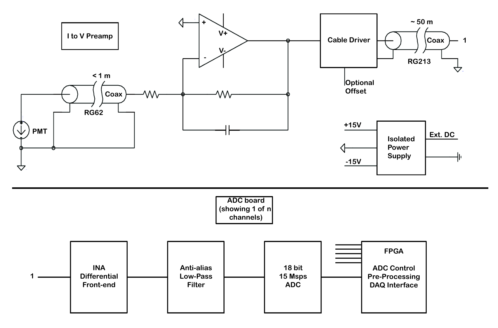
5.3.1 Integrating detector signal chain
The proposed P2 integration or current mode measurement front-end signal chain is shown in Fig. 49. The light from the quartz is converted to a current using quartz glass photomultiplier tubes (PMT) with a high quantum efficiency (QE) in the UV. At a nominal rate of 1 GHz and for a given detector geometry with a photo-electron yield of per primary electron, a mean current of roughly is produced at the anode of a PMT with a gain of about 1000. A trans-impedance preamplifier is used to convert the current signal to a voltage and to provide the primary filtering stage for the signal. The voltage signal is then further filtered and digitized by an ADC. Several channels of the filter and ADC chain are implemented on a single board, together with an FPGA, which queries the ADCs, collects (meaning in this case integrates) the data and facilitates the readout. The preamplifier also implements a line driver to sustain the signal over the longer cable distance between the detectors and the ADC. The preamplifiers and the integrating ADC boards are the main subject of this section.
The design of the electronics is, of course, dictated by the properties of the signal, including the mean amplitude, the RMS width, noise sources, and expected variation as a function of helicity. For the purposes of discussing the integrating electronics, the electronic signal from a single detector can be written as
| (69) |
This is the current that is present at the anode of the PMT, where is the contribution to the current from the physics process of interest (elastically scattered electrons and the secondaries they produce, indicated by the subscript ), the sum over is the contribution from the various background processes (indicated by the subscript ), and is the dark current (indicated by the subscript ). The current is converted to a voltage by an I-to-V amplifier with a gain of , in units of Ohms, so that the corresponding voltage yield is
| (70) |
Equation (70) includes a voltage contribution from a possible amplifier offset and the voltage signal corresponding to the dark current can contain helicity dependence due to possible electronic coupling of the helicity signal in the preamplifer. The latter should be suppressed or eliminated if possible through the use of appropriate signal isolation (avoidance of ground loops, signal isolation, the use of fiber optics, etc.).
For measurements in integration-mode, the counting statistics manifests itself primarily in the root-mean-square (RMS) width of the shot noise at the PMT anode, which has contributions from all sources that generate an anode current, including background and dark current. To get the total RMS width in the signal, as it is sampled by the ADC, one has to add all sources of electronic noise , which includes resistive (Johnson) noise, as well as noise introduced by active components and filters. The total squared RMS noise density in the signal is then given by
| (71) |
where is the mean anode current and is the mean quantum of charge at the anode. For the anode current this is simply a time average, but for the charge quantum the assumption is that this is the mean of a Poisson distribution and that the time integration for the current is done over a time period for which the quantum efficiency was stable. Note that, under ideal operating conditions, the dark current is dominated by thermionic emission of single electrons at the cathode, so that and the corresponding dark current is given by , where is constant depending on the cathode material and size, is the temperature in Kelvin, is the (field modified) work function of the cathode material, and is the Boltzmann constant.
In the expressions above, a possible, explicit dependence on helicity state of a given parameter is indicated by the superscript, while explicit time dependence (both slow and fast), that is generally not correlated with the helicity state is indicated by the continuous time parametrization . Aside from the physics asymmetries, the variation of various parameters with the helicity state of the beam may be a result of either electronic coupling of the helicity signal or direct variations in the beam as a function of helicity state. Examples of the former would be the coupling of the helicity gate into the signal that comes from the detector preamplifiers or the ADC electronics . Helicity correlated changes in beam conditions result in explicit changes of the rate seen in the detectors, even in the absence of any asymmetry that results from the interaction of the primary beam in the target or the rest of the experiment. Continuous time dependence in the detector signal is primarily due to variations in the beam current, target conditions, electronic drifts, temperature fluctuations, and PMT ageing, but also due to electronic drifts. A great deal of effort goes into the overall experimental design and analysis methods to remove or mitigate the dependencies on these unwanted experimental factors and many of the solutions are explicitly related to or influence the design of the integrating electronics.
5.3.2 Design criteria for the integrating electronics
The list below briefly describes the requirements the integrating electronics has to satisfy.
- 1.
Helicity correlated changes in the beam (current, energy, position, and angle) are unavoidable, but they can be minimized to some degree and they can be measured using charge and position monitors. The experiment will be designed to measure the sensitivity of the detectors to these beam changes. The sensitivity measurements are made by measuring the correlation between the changes measured with the beam monitors to those measured with the detectors, which requires that the electronics chain used to process the measurements from the beam monitors is identical to that of the integrating detectors. This is particularly important in the case of the beam current monitors, since the integrating detector signal is normalized to the current monitor signal to remove random drifts, fast fluctuations, and helicity correlated changes, in the beam current.
- 2.
Random and systematic drifts in the detector signal : The detector signal contains random changes and systematic drifts, both fast and slow. The slow drifts emerge due to variations in beam current, target conditions (target boiling and slower density changes), electronic drifts, temperature fluctuations, and PMT ageing. Almost all of these can be controlled to some degree (for example by operating the PMTs at a reasonable HV bias, in a reasonably stable temperature environment, and removed from or shielded from direct radiation exposure), but the primary way to deal with possible false asymmetries due to drifts and unwanted noise above shot noise, due to large amplitude random drifts, is to perform each asymmetry measurement on a timescale that is short compared to the timescale of the drifts. This is achieved by running the experiments with a fast helicity reversal rate (currently planned ) and a suitable choice of helicity patterns. Helicity quartets such as ++ and ++ remove linear drifts and the introduction of pseudo-random initial state () of the quartet removes quadratic drifts. The faster the helicity reversal rate, the more the signal variation with respect to time is well approximated as constant on the timescale of an asymmetry calculation:
Random variations that are faster than the helicity reversal rate are dealt with and used to advantage in the electronics chain, as described in detail below. The choice of helicity reversal rate influences or determines almost every detail of the electronics design.
- 3.
Minimization of electronics noise contribution:
- 4.
Minimization of drift effects and helicity correlated electronic pickup in the pedestal: .
- 5.
Minimization of drift effects and helicity correlated electronic pickup in the amplifier: .
- 6.
Bandwidth matching of all electronic components and between the various detectors that will be read out in integrating mode.
- 7.
Optimization of ADC resolution and sampling rate with respect to a reversal signal and the input bandwidth is required to follow (resolve) the helicity reversal signal transition (see below).
5.4 Signal structure and sampling scheme
Figure 50 shows a 2-minute period of the raw and beam current normalized signals for one of the QWeak integrating detectors. This data corresponds to an integration with an equivalent bandwidth of half the helicity reversal rate (), since the data for each helicity window is averaged to one value per helicity window, in the FPGA, after sampling. Even after normalization, drifts can be seen at timescales down to seconds, along with much longer drifts, and large non-Gaussian drops in yield, due to target boiling, can be seen at much shorter timescales (around ). A high helicity reversal rate prevents these types of drifts from producing false asymmetries and reduces the contribution to the RMS width in the asymmetry signal, due to these effects. For a mean signal of, say, a physics asymmetry of produces a shift in the mean of about , which is much smaller than the observed RMS width of a few . Since the bit resolution of even the best ADCs today is not high enough to measure a signal difference at that level, in a single sample, the combination of a suitable bandwidth selection and a high rate of oversampling is used to increase the effective bit resolution of the ADC.

Figure 51 illustrates the division of the integration mode detector signal into sampling regions. The period sampled for the physics measurement must be stable, which means that the time periods corresponding to the Pockels cell settling and ADC stability are excluded. However, it is important that the electronics be designed to allow sampling during the excluded time periods, so that the settling time can be monitored and used for systematic checks. The example in Fig. 51 shows the time structure used for the QWeak experiment, with a helicity reversal rate of , Pockels cell settling time of , and an ADC delay of . For P2, the reversal rate will be and the goal Pockels cell settling time is . This means that the integrating electronics settling should be correspondingly faster and operate at a higher sampling rate. The primary goal of the integrating electronics is to match the ADC bit resolution and sampling rate with the detector signal bandwidth needed to follow the changes in the beam (related to the helicity change and otherwise).
Figure 52 illustrates the concept behind the oversampling. The right hand side of the figure shows two simulated data sets (red and blue) for which the mean value differs (e.g., as a result of an asymmetry), as a function of sample time. The left hand side shows the samples accumulated by the ADC in histogram form. In this simulated data set, the mean difference between the two data sets is , while the bin width in the histogram, which represent the resolution of the ADC, corresponds to . Both of these values are exaggerated for illustrative purposes, but they show the general effect. The ADC resolution is too large to resolve the difference in the signal caused by the asymmetry, but the signal is sampled many times within each period (i.e., the helicity window) and the mean difference of the two distributions is clearly visible. This only works effectively, if the RMS width in the signal is significantly larger than the resolution of the ADC ( for an -bit ADC), which then automatically exceeds the digitization error in the ADC . Another benefit of the larger RMS width in the signal is that the ADC differential non-linearity becomes less and less significant while increasing the number of ADC channels over which the signal is spread. The experimental design and a suitable choice for the bandwidth in the preamplifiers and filters at the ADC input will ensure that this requirement is satisfied. The final ADC has to be chosen to have an integral non-linearity that is as small as possible, but since the difference in the mean of the signal for any pair of opposite helicity windows is smaller than the ADC resolution, the resulting distortions in the output distributions (left-hand panel in Fig. 52) for a given helicity pair will be nearly the same and the averaging over a large number of ADC bins, inherent in the this sampling scheme, reduces the effect further. For most good ADCs, the integral non-linearity as a function of ADC output code is distributed around LSB.

5.4.1 Bandwidth requirements
The lower limit to the system bandwidth is set by the need to follow the helicity flip settling time. The goal for the settling is and the front-end electronics has to be fast enough to follow this transition, to ensure that the amount of lost data within a helicity window is minimized. This means that the preamplifier output should also settle, within a certain accuracy relative to the mean helicity signal level, within a few . Taking a rate of in the detectors (approximately, from primary scattered electrons only), counting statistics within a single helicity window is about . Assuming that the noise from ringing during helicity transitions is perfectly correlated in all detectors and that we want the corresponding peak-to-peak variations to be much smaller than the counting statistics noise (shot-noise), we demand that the amplifier must settle to () within a time window that is small compared to the helicity flip settling time. A single pole filter with a signal bandwidth cutoff of has a time constant of and reaches the desired settling in , which is reasonable and also allows for some component variation and monitoring of additional ringing during the helicity transition. Suitable operational amplifiers for the preamplifiers have to be selected with these criteria in mind.
5.4.2 The preamplifier
The design of the P2 integrating electronics will be based on the QWeak electronics, but will be modified to satisfy, primarily, the criteria for higher bandwidth discussed above. The schematic for a single channel of the QWeak preamplifier is shown below, in Fig. 53. The inputs are protected with a combination of resistors and diodes. Each channel has a separate set of switches that set the gain between various values (here shown for QWeak, between and ). The bandwidth is primarily set by the parallel C1/R9 capacitor resistor feedback circuit, which was for QWeak. The displayed operational amplifier (OPA2604) can not support the desired bandwidth at the needed gains, so we will have to choose a different OpAmp, or implement a second gain stage. The constraints for the achievable signal bandwidth are set by the competing needs for the feedback capacitance (which controls the noise behavior), feedback resistance (which sets the overall gain), and the gain bandwidth product of the OpAmp. The two relevant relations are and , where is the desired signal bandwidth, is the gain bandwidth of the OpAmp (which is for the OPA2604 used for the QWeak design), and is the capacitance at the amplifier input, which is a combination of the OpAmp input capacitances, the PMT capacitance, and the cable capacitance. The latter two are, of course, dependent on the PMT base design and the cable length needed to connect the PMTs to the preamplifiers. The QWeak amplifier also implemented an offset control that sets an output bias voltage on each channel, to provide an indication that the preamp is powered and connected. An external 5V source powers an isolated DC-DC converter to supply internally.

5.4.3 The integrating ADC
As discussed in Sect. 5.4, two critically important parameters for the integrating detector ADCs will be the sampling rate and the amplitude or bit resolution. These are also competing parameters, in that ADCs with a high-bit resolution tend to have lower sampling rates and vice versa. Today, one can buy high performance, low noise, ADCs with 18 to 24 bit resolution and sampling speeds of several Msps. For P2, resolution is sufficient, given that the experiment will use the oversampling scheme described in Sect. 5.4. A suitable ADC has been identified11 1 Analog Devices http://www.linear.com/product/LTC2387-18, with a sampling speed of , which is significantly above the minimum required for the desired signal bandwidth.
For an event rate of , a PMT gain of 1000, and about 50 photo-electrons at the cathode, per event, the average current from a single detector would be about . Assuming also that the background and electronic noise contributions are negligible, Eq. (71) gives an estimated RMS width in the detector signal () of about (for a signal bandwidth). A preamplifier gain of would then produce a signal at the ADC, with a mean of and an RMS of about . The ADC currently under consideration has a full scale voltage range of and has a resolution of , which means that a signal with an RMS width of would be spread over more than channels, which is more than enough to make the digitization noise and non-linearity negligible, as discussed above.
5.4.4 Back-end data processing, readout, and DAQ interface
As illustrated in Fig. 51, the signal readout for the QWeak experiment included the option to split the signal into four blocks of consecutive samples, for diagnostic purposes, and this capability should be retained for the P2 design. In addition to this, it is desirable to implement the possibility to accumulate only every th sample in a given block, as illustrated in Fig. 54, primarily to monitor the effects of possible phase slippage between the integrating detectors and the beam monitors.

The QWeak design only allowed the readout of the sample sum for each entire helicity window and the sums for the four separate blocks within each helicity window. It is desirable to implement the readout of additional information in the data stream for each data block, such as the minimum sample value, maximum sample value, and RMS of the samples in each block. In addition, for diagnostic purposes, it is often desirable to obtain the fast Fourier transform of the actual signal, as it is sampled by the ADC. For this to work, it is necessary to implement the possibility of reading out every ADC sample, at a lower event rate (tracking rates), rather than only producing integrated numbers for each helicity window. This mode basically amounts to running the ADCs as slow waveform digitizers. This pre-processing of the ADC data will be implemented with an FPGA. For the purpose of commissioning, when the DAQ is being synchronized with the rest of the experiment, it will be necessary to have front panel outputs and data stream information about when exactly the FPGA starts and stops accumulating ADC samples after the helicity gate. The ADC will be controlled by an external clock that is synchronized to the helicity reversal. The ADC data will be read out via Gbit ethernet connections for each module.
5.5 Tracking detectors
Depending on the scattering position along the target, the solenoidal field will map different scattering angles into the acceptance of the integrating Cherenkov detectors. A tracking detector is needed to determine this relationship and ultimately the average squared momentum transfer of the electrons entering the asymmetry determination. High resolution tracking also allows for the study of backgrounds and position and momentum dependent systematic effects.
The tracking detector geometry and reconstruction was developed using a full Geant4 [91, 92, 93] based simulation of the P2 setup including a detailed field map based on the FOPI solenoid magnet [95].
5.5.1 Tracker operation modes
Two main modes of operation are foreseen for the tracker, one at low rates, where the Cherenkov detectors can be operated in single electron detection mode and coincidences with the tracker can be formed. A second mode at high rates is used to study rate, position and momentum dependent systematic effects; here the tracking detectors will be gated in order to keep the data acquisition rate manageable.
The first mode requires that the tracker acceptance at the very least covers all electrons that can reach one fused silica bar with very high efficiency, whilst the second mode demands a very fast, radiation tolerant detector with a geometry that allows for a reliable track reconstruction also at high occupancy. The low electron momentum and the reduction of background from photons created in the tracker put very stringent constraints on the tracker material budget.
5.5.2 Tracker geometry
The tracking detector uses the curvature in the magnetic field for momentum measurements, requiring placement in the solenoid and thus prevents a complete geometric shielding of the bremsstrahlung photons created in the target. Indeed, the first tracker plane is impinged by up to six orders of magnitude more photons than signal electrons. This in turn requires again a very thin tracker to minimize the photon interaction probability and a geometry that allows for a robust track reconstruction with a very adverse signal-to-background ratio of tracker hits (see Fig. 55). Such a robust track reconstruction can be achieved by tracking plane pairs spaced by roughly the typical distance of two hits on a single plane at full occupancy ( ).


For the low momentum tracks expected in P2, multiple Coulomb scattering in detector material is the main effect determining momentum resolution. It is thus desirable to have a long, material-free region to obtain a good curvature measurement. The demands of the reconstruction and good momentum resolution can be met by two double planes separated by a wide, empty drift region, the geometry chosen for P2, see the schematic view in Fig. 56.
The determination does not require full azimuthal coverage of the tracker; the active area should however be large enough to cover virtually all electrons heading for one fused silica bar. This can be achieved by tracker segments covering , see Fig. 57. We currently foresee four such segments to cover up-/down- and left-/right- asymmetries.
5.5.3 High-Voltage Monolithic Active Pixel Sensors
The P2 tracker requires active elements which are fast, thin, radiation hard and highly granular in order to deal with the high rates and low momentum tracks. High-Voltage Monolithic Active Pixel Sensors (HV-MAPS, see [99, 100, 101, 102, 103]) fulfill all these requirements. A commercial high-voltage CMOS process providing deep -wells in a -doped silicon substrate allows for reverse bias voltages of about between wells and substrate. This creates a thin, high-field depletion region, from which charge is quickly collected via drift. Inside the -wells, complete CMOS electronics can be implemented, allowing for in-pixel amplifier circuits and complete signal digitization and processing on the same chip. The thin active region allows for thinning of the sensors to just thickness.
In the framework of the Mu3e collaboration [104], we have developed a series of HV-MAPS prototypes known as the MuPix chips [105, 106]. With the MuPix7 prototype [107], we have produced a complete system-on-chip with a active pixel matrix with internal amplifiers and source followers, driving the signals to the chip periphery, where hits are detected by a tunable comparator and timestamps are assigned. A state machine collects and serializes the hits and sends them off-chip using a low-voltage differential signaling (LVDS) link. In this system, we have measured detection efficiencies well above and a time resolution below at noise rates below per pixel using a variety of beam tests at DESY, PSI, CERN and MAMI. High rate capability has been demonstrated by a MAMI beam test, where we illuminated a roughly large spot with more than of electrons, leading to an efficiency loss consistent with the single pixel deadtime of about , see Fig. 58. Despite no special design measures being taken, the sensors turn out to be very radiation hard [108].
Given the very large bremsstrahlung background expected in P2, it is imperative that the sensors have a small and well understood efficiency for detecting photons. To this end we have conducted tests with sources and at the A2 tagged photon facility at MAMI and find detection probabilities below for photons in the few MeV energy range, see Fig. 59. The detection probability rises again towards lower energies and was found to be at , again in good agreement with simulations [109].
We are currently testing the MuPix8 prototype in order to understand scaling effects in large sensors and prepare for the production of the final sensor.
5.5.4 Tracker segments
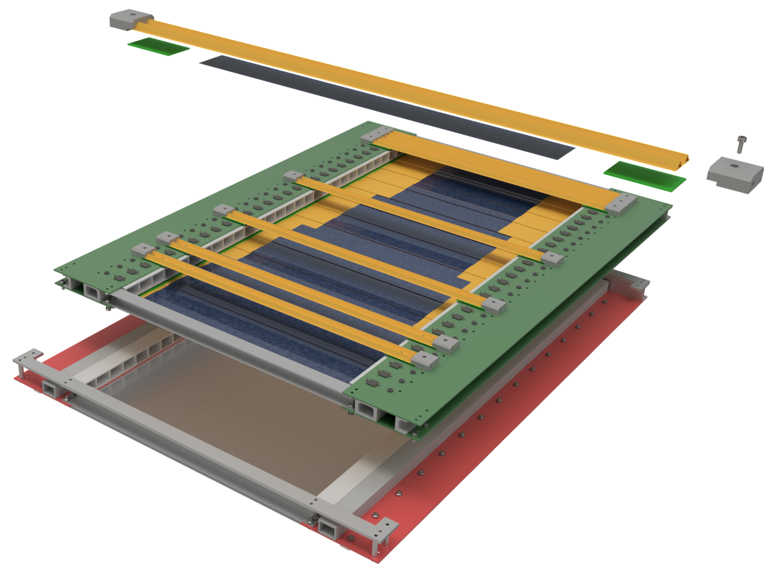
The tracker will consist of double layer segments covering in azimuth and as much as mechanically possible of the radial space between the Møller shield and the magnet inner wall ( to in radius). The active sensors will be cooled by gaseous helium.
Mechanics
A tracker module, see Fig. 60, is built from 29 staggered strips on each side with a slight overlap of the sensors along the radial axis to prevent ineffective areas and a frame providing mechanical support, cooling and electrical connectivity. Depending on the radius, each strip is equipped with between 8 and 14 thin HV-MAPS sensors, the strip design is derived from the Mu3e design [110]. About 30 single point tape-automated bond connections [111] to an aluminum-polymide flexprint provide the supply voltages and transfer data and control signals. An additional polymide layer with V-shaped folds glued to the flexprint provides mechanical stability and cooling channels. The overall thickness of the active part of a strip is less than of a radiation length.
The strip ends in a rigid printed circuit board (PCB) with a milled plastic cooling gas manifold on top; two different PCB thicknesses allow for the strip staggering. At both ends of the strip, these end PCBs are connected to a frame built from long PCBs and cooling ducts. Signals and power are connected via a high-density interposer. The azimuthal sides of the frame have a sliding system and are tensioned by springs in order to compensate for thermal expansion of the strips. Two layers of strips are connected to the same frame such that the sensors face inwards towards each other with a distance of roughly . The full module has 632 sensors.
The modules will be mounted on rails in their surrounding helium volume with the possibility to remove and re-insert them in a limited amount of time. This is in particular required for the runs with lead targets, where the radiation levels definitely exceed the tolerance of the tracker and gives the flexibility to also run without tracker in hydrogen mode in order to study systematics or perform repairs.
We are currently investigating two solutions for the powering of the HV-MAPS sensors, which require a supply voltage. Either this voltage is generated from an external supply via radiation hard DC-DC converters [112] mounted on the support frame or we employ a powering scheme, where several sensors are connected to the external supply in series; the required on-chip shunts are currently under test.
Cooling

The HV-MAPS sensors are active and, depending on their settings, dissipate between and . One module can thus produce in excess of of heat, which needs to be actively cooled; any liquid coolant would however add unacceptable amounts of material in the active region. We therefore employ a gaseous Helium cooling with high flows in the V-folds, the gap between the two planes in a module and over the module outside. Helium is suitable due to its long scattering length, high mobility and high speed of sound (allowing for large laminar flow speeds). The piping in the frame allows for counter-flowing helium streams in the two V-folds of each strip as well as on the top and bottom of a layer. We have performed extensive computational fluid dynamics simulations of the modules. With flow velocities of the initially Helium of in the V-folds and volume flows of in between and on top of the layers, a mean temperature of (maximum: ) can be achieved with heating power, see Fig. 61. The MuPix HV-MAPS sensors have been tested at temperatures above with only a very moderate amount of additional noise.
5.5.5 Tracker readout
At nominal beam current, the tracker produces in the order of of raw data, more than can be managed by an affordable readout system. We will thus use a gated mode, where the sensors are only active for short time slices.
The HV-MAPS sensors send out zero suppressed hit data (column and row address, time stamp) via a LVDS link with . The data are then sent out of the active volume either using radiation resistant LVDS repeaters or multiplexed on radiation hard optical links [113, 114, 115]. Both options are currently under study in terms of power and space requirements as well as signal integrity.
Outside of the radiation area, the signals are received by FPGA-based front-end boards. The data streams are synchronized and the hits time-sorted (the MuPix readout scheme introduces some randomization of the time-order of hits). The double plane structure of the tracker is then used to form hit pairs and thus reduce the data rate. These hit pairs are then forwarded to reconstruction PCs, where track finding and fitting is performed. The geometry of the P2 spectrometer and the limited momentum range of the tracks leads to a good locality of the tracking problem, reducing the need for complex data distribution networks.
5.5.6 Track reconstruction
Track finding.
The high occupancy of the tracking detectors at the nominal beam current makes track finding in P2 a potentially daunting task. We have developed an algorithm progressing from regions with low-occupancy to regions with high-occupancy using optimized track-dependent search windows [116] that elegantly manages the combinatorial problems posed. Figure 62 gives a schematic overview of the algorithm, which starts from the two tracking planes furthest away from the target and finds hit pairs consistent with a track from the target. The target constraint and the vector connecting the two hits are then used to define an optimal search window on the second plane of the front module. Matching hits found there are then validated using the front plane. Finally the four hits are subjected to a track fit (see below) and the fit is used to accept or reject the track. The performance of the algorithm in reducing the number of candidates reaching the fit state is shown in Fig. 63. The number of wrongly combined tracks (fakes) is highly dependent on the beam rate, see Fig. 64 but even at the full rate, a signal to background ratio above 10 can be achieved at a reasonable efficiency of .
Track fitting.
The best precision for the track parameters is obtained using a fit to the measured hit positions. We start by assuming that the track is a helix originating on the beam axis and passing through the centers of gravity of the first two and the last two tracker hits. This rough track, which assumes a constant magnetic field, is then used as a seed in the general broken lines fit [117, 118], which takes into account the hit position uncertainty and multiple Coulomb scattering at the two internal planes. The track state is propagated between planes using a Runge-Kutta-Nyström integration of the (inhomogeneous) magnetic field. From four 3D measurements, the fit determines two global track parameters (momentum and polar angle), eight shifts in the measurement planes and four scattering angle projections at the internal planes. The required additional constraints are the zero expectation value of the scattering angle and its variance from multiple scattering theory. In total there are 16 constraints and 14 fit parameters; the resulting track can be used to select well reconstructed tracks with little multiple scattering.
reconstruction.
For elastic scattering of a beam of known energy and direction, the momentum transfer can be determined from either the scattering angle or the outgoing electron momentum. The very long liquid hydrogen target in P2 however leads to energy losses and small angle scattering of both incoming and outgoing electrons, such that even a very good knowledge of the polar angle and momentum of the electron after leaving the target allows only a very approximate determination of . The distributions for energy loss, multiple scattering angles and detector acceptance are highly non-Gaussian and tend to cause biases, which is also the case for the radiative corrections to the large scattering (see Sect. 6.2). The reconstruction does thus have to rely on an iterative procedure using a Monte Carlo simulation including higher-order corrections, where not only the momentum and angle distributions, but also the longitudinal and radial position distributions of the point of closest approach need to be reproduced. We are still in the process of developing the respective algorithms and study potential sources of bias; currently we achieve a resolution per track of (), see Fig. 67. This allows us to reach the required statistical precision with a few dozen tracks — the measurement will be completely dominated by systematic uncertainties. We have started studying systematic uncertainties arising due to detector misalignment and estimate them to be much smaller than the required precision of after a track-based alignment. The dominating uncertainty is expected to arise from the MC description of multiple Coulomb scattering and energy loss in the target, which can only be addressed when beam data with the physical target become available. In the meantime, we will continue our efforts to qualify simulation models using test beam data, see e.g. [119].
6 Theory input
The interpretation of a high-precision measurement of the helicity asymmetry in ep scattering requires theory predictions with uncertainties below those of the experiment. In this section with describe the present status of the corresponding calculations.
To leading order in the electroweak coupling constants, the amplitude for elastic scattering of electrons with helicity is given by the sum of two Feynman diagrams which are due to the exchange of one photon and one boson, respectively,
| (72) |
While the exchange is parity-conserving, the exchange contains parity-violating contributions which flip sign depending on the helicity.
At very small elastic momentum transfer the internal structure of the proton is not resolved, and the two amplitudes only depend on the proton’s electric and weak charges, (in units of the positron charge) and , respectively,
| (73) |
with the mass of the boson and the weak mixing angle. The proton’s weak charge at tree-level is related to the weak mixing angle, .
The parity-violating asymmetry measures the difference between the cross sections for electrons with opposite helicities,
| (74) |
and for it is a small quantity which arises from the interference of virtual and exchange. Evaluating this asymmetry using Eq. (73) for very low and introducing the Fermi constant
| (75) |
we obtain
| (76) |
The direct proportionality between the PV asymmetry and the proton’s weak charge constitutes the basis of the P2 experiment.
To match the precision of the experimental measurement of , one has to go beyond the tree-level approximation and include radiative corrections described by Feynman diagrams with loops. They generically scale as , but may be enhanced by logarithms or large numerical factors, as, e.g., in the case of the box. Moreover, box diagrams are in general functions of two kinematical variables, and , which requires additional caution when relating the PV asymmetry to the proton’s weak charge.
The measurement of the PV asymmetry in PVES realized at finite energy and finite momentum transfer can be cast in the following form that generalizes Eq. (7) to include one-loop effects,
| (78) | |||||
where, for the sake of completeness, we keep the kinematically suppressed term introduced earlier in Eq. (7).
The one-loop SM result for has been formulated in Ref. [122] in the scheme, and Eq. (15) is replaced by
| (79) |
where is the weak mixing angle defined in the scheme at scale , where for the P2 experiment. In this equation, the Veltman parameter is a universal correction which renormalizes the ratio of the neutral and charged current strengths at low energies. and are small, non-universal corrections at the electron vertex. The term in Eq. (79) represents the contributions to from box graphs and is the subject of the next subsection.
The scale dependence of the weak mixing angle has been studied in Ref. [123] (see also [124] for a recent update). The value of at low momentum transfer is related by
| (80) |
to its value at the pole (with for the present values of the SM parameters).
In the scheme the scale dependence of the weak mixing angle is determined by the renormalization group evolution of the SM coupling constants. Other definitions of a scale-dependent effective weak mixing angle exist in the literature, see for example [125]. They are based on a redefinition of which absorbs universal and partly non-universal one-loop corrections into an effective weak mixing angle . Figure 68 shows some typical Feynman diagrams contributing to the scale dependence of the effective weak mixing angle.


6.1 Box graph and hadronic uncertainties
The one-loop result of Eqs. (78, 79) singles out the two-boson exchange contributions,
| (81) |
representative Feynman diagrams of which are displayed in Fig. 69. For each box graph, only the real part contributes and is understood as the real part of the corresponding diagram here and in the following. The box graphs are specific and have to be added as separate contributions since they depend on both the 4-momentum transfer and the electron energy. Other one-loop corrections depend on only and can therefore be factorized and partly absorbed into universal correction factors as shown above in Eq. (79).
It has been observed in Refs. [126, 127, 128] that the energy dependence of the heavy-boson box graphs associated with and exchange induces corrections of order , rather than . For electron energies up to a few GeV these energy-dependent contributions can be safely neglected. The constant terms, however, are numerically large. Since they are dominated by contributions from loop momenta of the order of , their calculation in the framework of perturbation theory is safe with a reliable uncertainty estimate [122].
The box does not contain large logarithms and is known to vanish at small momentum transfer as it can only renormalize the charge radius of the proton but not its charge. Since it only corrects the parity-conserving part of the amplitude, its effect on the PV asymmetry will also be multiplied by the proton’s weak charge. All in all, it is natural to expect a correction to of the order of due to -box graphs. This amounts to a negligible correction of order for the kinematical conditions at the P2 experiment that can be accommodated in the uncertainty associated with the kinematically suppressed correction term . With these observations, the energy dependence of the boxes present in Eq. (78) reduces to that of the box,
| (82) |
The -box graph contains a large logarithm where is a typical hadronic mass scale. The coefficient in front of this large logarithm is energy-independent up to corrections and can be calculated precisely using quark sum rules [126, 127]. The presence of the hadronic mass scale signals the sensitivity of the box to the hadronic structure, and this sensitivity was used to estimate the hadronic structure-related uncertainty [122]. However, early studies described in the references given above had assumed that the energy dependence of the box was negligible, , following the pattern of the heavy boson boxes.
Subsequently, the energy dependence of the box was addressed in Ref. [129] in the framework of forward dispersion relations. It was shown that the energy dependence of is much more significant than anticipated. It has been the subject of active scrutiny in the theory community [120, 130, 131, 132, 57, 133]. The dispersive method for calculating is per se model-independent, relating the box to an integral over measurable unpolarized interference structure functions . Nonetheless, due to the lack of reliable experimental data for these structure functions one is forced to introduce model assumptions to define the required input in unmeasured regions. While different groups agree on the central value of within errors, this model dependence leads to a discrepancy in the uncertainty estimate.
In Fig. 70 the energy dependence of the box is shown. It is obtained as a sum of its vector part calculated in Ref. [57] and its axial-vector part, obtained in Ref. [134, 132, 135] at zero momentum transfer. The respective uncertainties are added in quadrature. The extrapolation from the actual value of corresponding to the kinematics at P2 down to is done according to Ref. [120]. Due to the tiny value of GeV2 this extrapolation leads to a numerically negligible effect, both on the central value and its uncertainty. For the kinematics at P2, the energy-dependent contribution amounts to
| (83) |
and the uncertainty is dominated by that due to the effective axial charge of the nucleon seen by charged leptons, also referred to as the anapole moment,
| (84) | |||||
| (85) |
A measurement at backward angles as described in section 7.3 will allow to reduce the uncertainty due to the anapole moment considerably, . Assuming that this precision goal is achieved, the energy-dependent correction from the box will change to
| (86) |
with a reduced uncertainty. This estimate was used in Sect. 2, Tab. 2 in the summary of the uncertainty budget.
6.2 QED corrections
Electromagnetic corrections are parity conserving and do not affect the proton’s weak charge. However, the relation to the measured helicity asymmetry receives corrections since extra radiated photons lead to a shift of the observed momentum transfer relative to the true one. can not be determined from the electron scattering angle alone, but the momentum of unobserved photons has to be taken into account.
The tracking detectors described in Sect. 5.5 will allow one to determine the momentum of the scattered electron, i.e., its energy and the electron scattering angle . From this information one can determine (corresponding to Eq. (6)), where and are the momentum 4-vectors of the initial and final electron. In the presence of bremsstrahlung, a photon with 4-momentum emitted from the electron will shift to the true momentum transfer . This true value has to be used in the equation relating the measured asymmetry with the proton’s weak charge, Eq. (7).

In Fig. 71 we show the average relative shift of due to photon radiation including one-photon bremsstrahlung. The shift depends strongly on the beam energy and the scattering angle, as well as on a possible cutoff of the energy of photons radiated into the final state. Preliminary results of a calculation including two-photon radiation show that order corrections are much less important. This can be understood since we deal with a kinematic effect: the relation between scattering angle and momentum transfer is not unique anymore in the presence of an additional photon. A second photon does not add considerably more freedom, but only adds corrections of order to the cross section. Eventually, bremsstrahlung effects will be included in the detector simulation.
6.3 Theory summary
The current SM prediction for the parity-violating asymmetry in elastic ep scattering, summarized in this section, includes the complete set of NLO corrections. At this order, no further theoretical uncertainties will affect the interpretation of a high-precision measurement of in terms of beyond the level of . In particular, uncertainties from the hadronic structure entering the -box graph at the low energy and small values relevant for the P2 experiment are well under control.
A conclusive test of the SM and analyses of the anticipated experimental result at P2 in terms of New Physics can be obtained by comparing with other high-precision determinations of the weak mixing angle from LEP, SLC, and future measurements at the LHC. This will require the inclusion of two-loop electroweak corrections and work on the corresponding NNLO calculations is underway.
7 Further physics programme
7.1 Measurements with Carbon-12
High precision measurements of the weak charges of different particles and nuclei offer complementary sensitivities to physics beyond the Standard Model in the form of new tree level and quantum loop correction parameters. For example, one may consider ratios of polarization asymmetries in which the polarization uncertainty mostly cancels.
Here we summarize the results of first feasibility studies of a measurement of the weak charge of the 12C nucleus with the P2 setup. As a spin-zero nucleus, 12C can be described by a single form factor and is thus theoretically easy to handle [8]. Moreover, its QED cross section is 36 times larger than that of the proton, and its weak charge is 78 times as large, which significantly reduces beam time requirements. The SM prediction for the helicity asymmetry at leading order can be written as in Eq. (7) with
| (87) |
At low momentum transfer weak charges can be parametrized with respect to the so-called oblique parameters, such as the , and parameters introduced by Peskin and Takeuchi [136, 137]. However, , and are already very precisely determined from -pole observables, whereas weak charges are able to constrain some of the higher-order oblique parameters. For example, the parameter [138] describes the difference of new physics contributions to the mixing at the pole and at low energies, and cannot be determined by -pole physics alone. Likewise, in the absence of mass mixing, -pole observables are virtually blind to extra heavy gauge bosons as new amplitudes are suppressed relative to the resonance. By contrast, at low energies amplitudes are merely suppressed by the square of the ratio of the and masses. One has [44]
| (88) |
for the weak charges of , the proton, the electron and , and was used where is the extra boson predicted by Grand Unified Theories (in the absence of gauge kinetic mixing). The different pre-factors in this parametrization show the complementarity of the different weak charges to physics beyond the Standard Model. Low- measurements also have unique sensitivity to certain beyond the Standard Model scenarios such as those involving so-called dark bosons [139], which are light (on the order of tens of MeV) and very weakly coupled extra neutral gauge bosons which may mix with the ordinary boson, and which may be parametrized by taking as a function of .
One can also discuss the implications of weak charges in a model-independent way. In the effective field theory picture, the Standard Model may be defined by the most general Lagrangian consistent with gauge and Lorentz invariance built from the known particles up to dimension four, while the weak charges probe specific (combinations of) dimension six operators. In photon-interference experiments only vector and axial-vector Lorentz structures are important, and in the elastic regime the nucleus couples vector-like and parity-violation then forces the electron to enter axial-vector-like. Constraints on the quark-vector and electron-axial-vector couplings are illustrated in Fig. 72.
7.1.1 Achievable precision
The achievable precision of was determined numerically as described in section 2.2.1. The underlying Eqs. (18) and (19) have been modified appropriately for the case of scattering with a target. The beam energy was varied in the range from to , and we used a beam current of , a data taking time of , and for detector acceptance angles between and . We assumed a beam polarization of with a relative error of .
Figure 73 shows the achievable precision for a fixed beam energy of and an acceptance angle of as a function of the average scattering angle . It demonstrates that the total error in is dominated by the contribution of the beam polarization uncertainty (cyan) rather than by the statistical error (green).
Figure 74 summarizes the minimum values for the total error in for all simulated beam energies and scattering angles. It shows that we can obtain a relative error of 0.3 % with high detector acceptance angles and beam energies of . As the weak charge of the 12C nucleus is proportional to , this corresponds to a relative error in the weak charge of 12C of 0.3 %.
7.1.2 Experimental setup
For the 12C experiment, the P2 hydrogen target in Fig. 19 can be replaced by a 5-finger graphite target to ensure high luminosities while suppressing double scattering inside the target.

In order to find a suitable spectrometer, detector, and collimator setup, a Geant4 ray tracing study was carried out. Figure 75 shows the distance of the electron trajectories from the beam axis . Such plots were created for a variety of target positions and for spectrometer magnetic fields ranging from 0.1 T to 1 T. When studying the results of the simulation, a setting with which we can place the detector at a focal point of the electrons of interest and with which the undesired background can be collimated was sought. Possible detector and collimator positions are included in Fig. 75.
Furthermore it is crucial to sort out inelastically scattered electrons. The plot in Fig. 76 shows the trajectories from elastically scattered electrons with a beam energy of in red. Trajectories of the electrons that have excited the nucleus to the first and second excited states are shown in blue and yellow, respectively. In these cases, the energy of the electrons is effectively reduced to (for the first excited state) or (for the second excited state). The simulations show that the trajectories are well separated in all cases.
7.1.3 Conclusion
A measurement of the weak charge of the 12C nucleus at MESA can be made with a relative precision of 0.3 % assuming a measurement time of one fourth of that for P2 with a proton target. This corresponds to a precision in the weak mixing angle of 0.3 %. The 12C experiment will provide additional and complementary sensitivity to certain classes of new physics models. Furthermore, already individually the carbon and proton measurements by P2 will provide the strongest constraints (95% CL sensitivities of around 50 TeV in strong coupling scenarios [55]) on any CP-allowed four-fermion operator built from first generation fermions. Combined, the operator corresponding to the coupling combination along the minor axis of the red ellipse in Fig. 72 would be probed up to . First conceptual studies regarding the feasibility of the project give promising results.
7.2 Neutron skin measurement
High precision parity-violating electron scattering experiments on nuclei provide a portal to the properties of neutron-rich matter. Unfortunately, it is difficult to study neutron matter directly in the laboratory because the neutron and extremely neutron-rich isotopes are unstable. However, heavy nuclei are expected to develop a neutron-rich skin where many neutrons collect near the surface. Since the parity-violating asymmetry is particularly sensitive to the neutron density, it provides a clean and model independent measurement of the neutron skin of nuclei.
The neutron-skin thickness of a nucleus , defined as the difference between the neutron and proton rms-radii is strongly related to the poorly-known symmetry energy at saturation density . The symmetry energy is a key parameter of the nuclear Equation of State (EoS) [140], since it quantifies the changes in nuclear energy associated with modifications of the neutron-proton asymmetry. It determines as well the properties of spectacular astrophysical phenomena such as supernovae explosions or neutron star mergers.
After the first observations of two colliding neutron stars [141], the emergent multi-messengers astronomy field will provide us with new ways to constrain the EoS and the properties of neutron-rich matter. Even stronger constraints can be imposed by combining this information with independent measurements like the precise determination of the neutron-skin thickness of heavy nuclei.
Though intensive experimental effort has been made to determine the neutron-skin thickness, a precise measurement of this quantity remains elusive. Several observables sensitive to the neutron skin have been proposed and recent experiments have been successful in measuring giant- and pygmy-resonance modes [142] on a variety of nuclei as well as the electric-dipole polarizability [143] and coherent pion photoproduction [144]. These data together with data from hadron scattering experiments (involving protons [145], anti-protons [146] and pions [147]) are valuable, but interpretations contain implicit model dependences.
The measurement of parity-violating asymmetries provides a clean and model-independent determination of neutron-skin thicknesses. In Born approximation the parity-violating asymmetry is proportional to the weak form factor ,
| (89) |
is the Fourier transform of the charge density which is known. A measurement of the parity-violating asymmetry will therefore allow one to determine the weak-charge density , from which the weak radius
| (90) |
and thus the neutron radius can be obtained. Taking the known charge radius into account, the neutron-skin thickness can be determined, for details see Refs. [148, 149]. The 208Pb Radius EXperiment (PREX) at JLab has provided the first proof-of-principle of the application of parity-violating electron scattering for the measurement of the neutron-skin thickness [46]. The experiment achieved the systematic error goals of and was a major accomplishment as a first measurement of its kind. However, because of various problems, the experiment took only of the planned statistics. With all corrections, the measured asymmetry is ppm at = 0.00906 GeV2. This corresponds to a value for the neutron skin of 208Pb of fm and confirmed the existence of a neutron-radius excess with a 2 statistical significance.
The P2 experiment will open the window for a new generation of high-precision parity-violating electron-scattering experiments. Within the scope of the P2 experimental setup, the Mainz Radius EXperiment (MREX) will determine the neutron-skin thickness of 208Pb with ultimate precision. Figure 77 shows the expected cross section, parity-violating asymmetry, and sensitivity as well as the resulting figure of merit (FOM) for a beam energy of .

Here, the relevant figure of merit for a neutron skin measurement, for a given energy, is:
| (91) |
In addition to the typical FOM for parity-violation experiments, the sensitivity of to changes in the neutron radius was taken into account [148]:
| (92) |
To estimate the best possible achievable precision with MREX, calculations within the peak sensitivity in the polar angular range have been performed using three different settings for the detector acceptance: and . A beam polarization of at least and a systematic uncertainty of in the determination of was taken into account for the calculation. Compared to the given error contribution in Tab. 2, a rather conservative estimation for the size of the systematic uncertainty was used. The best sensitivity was obtained with a detector acceptance of in the angular range between and . The running time for the latter one was restricted to 2500 hours to fit the overall beam-time planning of the MESA accelerator. Already after 1500 hours a determination of the neutron radius with a sensitivity of can be achieved (see Fig. 78). The main parameters used for the calculation are summarized in Tab. 15.

| Beam energy | |
|---|---|
| Beam current | |
| Target density | |
| Polar angle step size | |
| Polar angular range | to |
| Degree of polarization | |
| Parity-violating asymmetry | |
| Running time | 1440 hours |
| Systematic uncertainty | |
A crucial requirement for the experiment to correctly measure the parity violating asymmetry is the separation of the ground state of 208Pb from its first excited state (). Therefore tracking simulations of signal and background particles in the angular range of interest ( to ) have been performed for a solenoid with a magnetic field strength of . For this study the existing trajectory simulation (see Sect. 5.1.3 for details) was adapted and the extended hydrogen target was replaced by a point-like lead target. Trajectories were calculated for the elastically scattered electrons with an energy of as well as for electrons with an energy of , mimicking events from the first excited state of 208Pb. The target position was varied between and using a step size of . With two configurations it was possible to get a clean separation between the elastic and inelastic events. The two options with the target placed at and are illustrated in Fig. 79 and Fig. 80, respectively.


In both cases it is possible to block the inelastic events with a set of collimators. While both options need the same amount of space behind the solenoid to position the detectors, option II requires additional space in front of the solenoid, adding a further experimental requirement to the changes in the P2 hall. Moreover, option I is similar to the detector configuration intended for the measurement of the weak mixing angle and could allow the use of a combined scattering chamber. This would simplify the structural alteration works during the two experimental campaigns. Implementation of the lead target inside the planned scattering chamber as well as a more detailed Geant4 simulation, including radiative corrections, are currently being performed to finalize the design.
The preliminary results reported here show that a measurement () of the neutron skin thickness of 208Pb using the P2 setup is feasible.

Figure 81 shows the predicted MREX sensitivity together with the first calculation of the tidal deformability parameter of two spiraling neutron stars observed by LIGO [141] as a function of the neutron skin thickness of 208Pb within different density functional models. Of course such correlations are only approximate since the neutron skin in 208Pb depends on the EoS at about , while the radius of a neutron star and its deformability depend on the EoS at about twice the nuclear density. However, in general the higher the pressure at low density the larger the skin and the higher the pressure at higher densities the bigger the deformability. The upper bound observed by LIGO is consistent with rather thin neutron-skin thicknesses. The future PREX-II experiment at JLab [151] with its anticipated precision of together with additional measurement of neutron star mergers at LIGO will clarify the current picture.
Moreover, the improvement in accuracy aimed for by the MREX will provide stringent constraints to such correlation and thus lead to a deeper understanding of neutron-rich matter.
7.3 Backward angle measurement
As seen in Eq. (7), the parity-violating asymmetry depends not only on the weak charge of the proton, but also on its hadronic structure. Since , a measurement at low momentum transfer GeV2 is mainly sensitive to the weak charge . Nevertheless, for any the hadronic contribution cannot be neglected. can be split up into the three terms , and , see Eqs. (8-11). In order to extract the weak charge, the term does not limit the achievable precision because the electromagnetic form factors are known at sufficiently high precision. On the other hand, the axial form factor and the strange magnetic form factor have relatively large uncertainties such that the terms and make non-negligible contributions to the uncertainty, depending on the scattering angle or the momentum transfer respectively. Therefore we plan a dedicated measurement of these form factors within the P2 experiment. A backward-angle measurement is much more sensitive to and compared to a measurement at forward angles. Two different scenarios can be considered: either a backward-angle measurement in parallel to the main forward-angle experiment or dedicated measurements at backward angles alone. The first option depends on the available space in the experimental hall as well as on the availability of additional detectors, readout etc. The second option would require additional beam time in the order of .
| P2 backward-angle experiment | |
|---|---|
| Integrated luminosity | |
| Statistical uncertainty | ppm |
| False asymmetries | ppm |
| Polarimetry | ppm |
| Total uncertainty | ppm |
A backward-angle measurement parallel to the main experiment could be done in principle for the whole experiment time, i.e., . The beam energy used for the following discussion is . The backward detector covers polar and azimuthal scattering angles of and , the momentum transfer is GeV2. Table 16 shows what could be achieved with such a P2 backward-angle measurement. One can see that the asymmetry could be measured to a precision at the sub-percent level with the beam polarization as the main source of uncertainty. From this asymmetry, one can derive a value for the linear combination:
| (93) |
Here, the form factor input is the predominant source of uncertainty. For the P2 forward measurement, one needs as input the linear combination . If one scales down the linear combination from the backward-angle measurement to the P2 forward conditions, one has to keep in mind that the linear combinations are slightly different and the momentum transfers do not match exactly. Therefore we add an additional error for this transformation of of the error of the measured linear combination. The benefit of the backward-angle measurement can be clearly seen: The uncertainty which is used as an input to the P2 main experiment analysis drops from if no backward-angle measurement is performed down to using the results of the backward-angle measurement. This would mean an improvement by a factor of 4.
We also considered two dedicated backward-angle measurements with of data taking each using a hydrogen and a deuterium target. The beam energy for this calculation is , which corresponds to a momentum transfer of GeV2. Combining hydrogen and deuterium results, one could obtain and separately, which is a valuable physics result by itself.
In order to estimate the achievable precision in and , all quantities that enter into their determination were varied according to their uncertainties. The width of the distributions are displayed in Fig. 82 and Fig. 83. It turns out that the possible uncertainties would be and . The impact on the forward P2 experiment would be even better compared to a parallel backward-angle measurement, because the momentum transfer would match better and the required linear combination can be calculated directly from the separated form factors.
To conclude, backward-angle measurements within the P2 experiment seem promising. Two options were discussed. A backward-angle measurement parallel to the forward P2 experiment doesn’t require additional beam time, but depends on the available space in the experimental hall. The uncertainty contribution of axial and strange magnetic form factors, expressed by would drop by a factor of 4 compared to the assumptions without such a measurement. Separate measurements on hydrogen and deuterium targets seem even more promising and would yield the most precise determination of and at low momentum transfer.
8 Conclusions and Outlook
This work summarizes the research and development work for the P2 experimental facility at the upcoming energy recovering recirculating accelerator MESA in Mainz. It is optimized for the measurement of an order 10-8 parity-violating cross section asymmetry in electron scattering. This is the smallest asymmetry ever measured in electron scattering. Many new experimental techniques will be used for the first time in order to reach the high precision goal needed to obtain physics results with a high impact on the field of research. These are:
-
a superconducting solenoid as a spectrometer for scattered electrons;
-
HVMAPS as thin silicon tracking detectors for the measurement;
-
a so called Hydro-Møller polarimeter, a magnetic trap for Møller scattering off atomic hydrogen;
-
a low energy recirculating accelerator with low number of recirculations and energy recovery capability.
The P2 experimental facility has a rich program covering different fields like particle physics and nuclear physics. The building hosting the MESA accelerator will be finished according to the present construction plan in mid of 2020. The start of the accelerator and experiment commissioning is foreseen mid of the year 2021. A detailed beam-time plan for the experimental program has not yet been set up. This needs to be discussed in order to achieve a good compromise between commissioning of MESA and P2 and the high demands of the parity-violation program. Ideally, one would run experiments with large asymmetries and short measurement times first in order to meet the increasing demands of the experiments in parallel to the performance increase achieved by careful commissioning of accelerator, beam control systems, polarimetry and experimental setup. The present physics topics of P2 identified as topics with a high impact on the respective research fields, are:
-
Measurement of the weak charge of the proton for the determination of the weak mixing angle with an accuracy of . The expected asymmetry is , averaged over cross section and acceptance. The necessary measurement time is . This is the most demanding measurement due to the small size of the asymmetry and the long measurement time. The target accuracy will go beyond the present state of the art by a factor three, corresponding to a factor of 10 higher statistics and a factor of three higher in all beam-related apparative asymmetries, and polarimetry on the level of 0.5%. It has a sensitivity for new physics beyond the standard model with mass scales ranging from up to and complementary to the new physics searches at the LHC.
-
Measurement of the weak charge of the 12C nucleus. The asymmetry is of order due to the large weak charge of the neutrons in 12C and the measurement would need about . The precision goal of is a challenge for polarimetry and requires additional research and development work. In combination with the measurement of the weak charge one can reach a still higher sensitivity for new physics of mass scales up to about .
-
Measurement of the neutron skin of the 208Pb nucleus. The asymmetry is of order and the measurement would need about . The result is expected to yield an error on the neutron radius of of . Such a measurement will be important for a better understanding of the physics of neutron stars.
-
A backward-angle measurement of the parity-violating elastic scattering to measure the weak form factor of the nucleon. From measurements with hydrogen and deuterium targets, the error bars for and can be reduced substantially.
The experimental program described in this manuscript comprises several years of pure data taking, calibration and the study of systematic effects like a parity-violating asymmetry from the aluminum windows. Together with the beam-time demand from the second MESA flagship facility MAGIX, one can safely say that we are facing 6 to 10 years of a research program at MESA.
Technically, the beam energy of MESA could be increased up to . The discussion of a possible research program for this enhanced MESA setup is ongoing. It would bring the pion-production threshold, both for scattering off protons and for heavier nuclei, into the reach of the experimental facilities at MESA. In particular the study of hadronic parity violation which has seen enormous progress in the theory sector over the last years will be interesting [152, 153].
At energies above the pion production threshold, it is possible to directly address hadronic parity violation effects, in particular the parity-violating coupling constant . As pointed out in Refs. [154, 155] these effects become prominent in the near-threshold charged pion production with a polarized electron beam and with only the charged pion in the final state detected. The origin of this parity-violating coupling lies in the effective four-quark operators which are also responsible for generating the anapole moment. The anapole moment is the source of the largest uncertainty in the upcoming P2 experiment. Furthermore, measuring the parity-violating asymmetry in inelastic electron scattering between the pion production threshold and the resonance, as argued in Ref. [57], offers an enhanced sensitivity to strange form factors of the nucleon.
Finally, the increased energy reach of MESA with a polarized beam
would make it possible to perform a new measurement of the
parity-conserving, beam normal spin asymmetry in elastic ep
scattering at backward angles. This observable is a single-spin
asymmetry with the electron polarization normal to the scattering
plane. It is a purely electromagnetic effect which contributes an
important systematic uncertainty to parity-violating electron
scattering. The earlier measurement at and
at MIT-Bates [12] are not fully understood: the
observed large asymmetry is at variance with the much smaller
theory expectation [156] which is, at this
energy, essentially free of uncertainties.
The upcoming new Mainz P2 experimental facility will bring very interesting times in the measurement of parity violating electron scattering.
9 Acknowledgements
This work is supported by the Deutsche Forschungsgemeinschaft
(DFG) in the framework of the collaborative research center
SFB1044 “The Low-Energy Frontier of the Standard Model: From
Quarks and Gluons to Hadrons and Nuclei”, and in the
framework of the PRISMA cluster of excellence “Precision
Physics, Fundamental Interactions and structure of Matter”.
Silviu Covrig acknowledges support by an Early Career
Award from the DOE.
Jens Erler acknowledges support in part by the German-Mexican
research collaboration grant 278017 (CONACyT) and SP 778/4-1
(DFG), as well as by CONACyT project 252167-F.
Michael Gericke is partially supported by funding received
through the Natural Sciences and Engineering Research Council
of Canada (NSERC) and the Canadian Foundation for Innovation
(CFI).
Mikhail Gorchtein acknowledges support by the DFG under the
personal grant GO 2604/2-1.
Boxing Gou would like to thank the Office of China Postdoctoral
Council (OCPC) for financial support.
The P2 tracker group would like to thank the Mu3e group in
Heidelberg, in particular Frank Meier-Aeschbacher and Dirk
Wiedner for many helpful discussions.
This work comprises part of the Phd thesis work of Dominik
Becker, Razvan Bucoveanu, Carsten Grzesik, Ruth Kempf,
Kathrin Imai, Matthias Molitor, Alexey Tyukin, and Marco
Zimmermann.
Appendix A Nucleon form factor fit parameters
It has been assumed in Eq. (21) that the nucleon form factors can be parametrized as functions , where is a set of independent, real parameters. The parametrizations used are discribed in Sect. 2.2.2. Here we present the expected values and standard deviations of the parameters , which have been used in the error propagation calculations.
| i | / | / |
|---|---|---|
| 1 | ||
| 2 | ||
| 3 | ||
| 4 | ||
| 5 | ||
| 6 | ||
| 7 | ||
| 8 |
| / | / | |
|---|---|---|
| 1 | ||
| 2 | ||
| 3 | ||
| 4 | ||
| 5 | ||
| 6 | ||
| 7 | ||
| 8 |
| i | ||
|---|---|---|
| 1 | ||
| 2 |
| i | / | / |
|---|---|---|
| 0 | ||
| 1 | ||
| 2 | ||
| 3 | ||
| 4 | ||
| 5 | ||
| 6 | ||
| 7 | ||
| 8 | ||
| 9 |
| i | ||
|---|---|---|
| 1 | ||
| 2 |
| i | / | / |
|---|---|---|
| 0 | ||
| 1 |
| i | / | / |
|---|---|---|
| 0 | ||
| 1 |
| i | / | / |
|---|---|---|
| 0 | ||
| 1 | ||
| 2 | ||
| 3 | ||
| 4 |
| i | / | / |
|---|---|---|
| 0 | ||
| 1 | ||
| 2 | ||
| 3 | ||
| 4 |
References
- (1) T. D. Lee and C.-N. Yang, “Question of Parity Conservation in Weak Interactions”, Phys. Rev., 104 254–258, 1956.
- (2) C. S. Wu, E. Ambler, R. W. Hayward, D. D. Hoppes and R. P. Hudson, “Experimental Test of Parity Conservation in Beta Decay”, Phys. Rev., 105 1413–1414, 1957.
- (3) R. L. Garwin, L. M. Lederman and Marcel Weinrich, “Observations of the Failure of Conservation of Parity and Charge Conjugation in Meson Decays: The Magnetic Moment of the Free Muon”, Phys. Rev., 105 1415–1417, 1957.
- (4) Ya. B. Zeldovich, “Parity nonconservation in the first order in the weak interaction constant in electron scattering and other effects”, Sov. Phys. JETP, 36 964, 1959.
- (5) C. Y. Prescott et al., “Parity Nonconservation in Inelastic Electron Scattering”, Phys. Lett., B77 347–352, 1978.
- (6) M. A. Bouchiat, J. Guena, L. Hunter and L. Pottier, “Observation of a Parity Violation in Cesium”, Phys. Lett., 117B 358, 1982, [Erratum: Phys. Lett.121B,456(1983)].
- (7) W. Heil et al., “Improved Limits on the Weak, Neutral, Hadronic Axial Vector Coupling Constants From Quasielastic Scattering of Polarized Electrons”, Nucl. Phys., B327 1–31, 1989.
- (8) P. A. Souder et al., “Measurement of parity violation in the elastic scattering of polarized electrons from C-12”, Phys. Rev. Lett., 65 694–697, 1990.
- (9) D. B. Kaplan and A. Manohar, “Strange Matrix Elements in the Proton from Neutral Current Experiments”, Nucl. Phys., B310 527–547, 1988.
- (10) B. Mueller et al., [SAMPLE], “Measurement of the proton’s neutral weak magnetic form-factor”, Phys. Rev. Lett., 78 3824–3827, 1997, (arXiv:nucl-ex/9702004).
- (11) D. T. Spayde et al., [SAMPLE], “Parity violation in elastic electron proton scattering and the proton’s strange magnetic form-factor”, Phys. Rev. Lett., 84 1106–1109, 2000, (arXiv:nucl-ex/9909010).
- (12) S. P. Wells et al., [SAMPLE], “Measurement of the vector analyzing power in elastic electron proton scattering as a probe of double photon exchange amplitudes”, Phys. Rev., C63 064001, 2001, (arXiv:nucl-ex/0002010).
- (13) R. Hasty et al., [SAMPLE], “Strange magnetism and the anapole structure of the proton”, Science, 290 2117, 2000, (arXiv:nucl-ex/0102001).
- (14) D. T. Spayde et al., [SAMPLE], “The Strange quark contribution to the proton’s magnetic moment”, Phys. Lett., B583 79–86, 2004, (arXiv:nucl-ex/0312016).
- (15) T. M. Ito et al., [SAMPLE], “Parity violating electron deuteron scattering and the proton’s neutral weak axial vector form-factor”, Phys. Rev. Lett., 92 102003, 2004, (arXiv:nucl-ex/0310001).
- (16) F. E. Maas et al., [A4], “Measurement of strange quark contributions to the nucleon’s form-factors at = 0.230 (GeV/c)2”, Phys. Rev. Lett., 93 022002, 2004, (arXiv:nucl-ex/0401019).
- (17) S. Baunack et al., [A4], “Realtime calibration of the A4 electromagnetic lead fluoride calorimeter”, Nucl. Instrum. Meth., A640 58–68, 2011, (arXiv:1102.5640 [nucl-ex]).
- (18) P. Achenbach et al., “Radiation resistance and optical properties of lead fluoride Cherenkov crystals”, Nucl. Instrum. Meth., A416 357–363, 1998.
- (19) P. Achenbach, S. Baunack, K. Grimm, T. Hammel, D. von Harrach, A. Lopes-Ginja, F. E. Maas, E. Schilling and H. Stroher, “Measurements and simulations of Cherenkov light in lead fluoride crystals”, Nucl. Instrum. Meth., A465 318–328, 2001, (arXiv:nucl-ex/0108019).
- (20) F. E. Maas et al., “Measurement of the transverse beam spin asymmetry in elastic electron proton scattering and the inelastic contribution to the imaginary part of the two-photon exchange amplitude”, Phys. Rev. Lett., 94 082001, 2005, (arXiv:nucl-ex/0410013).
- (21) F. E. Maas et al., “Evidence for strange quark contributions to the nucleon’s form-factors at q**2 = 0.108 (GeV/c)**2”, Phys. Rev. Lett., 94 152001, 2005, (arXiv:nucl-ex/0412030).
- (22) T. Hammel et al., “A Luminosity monitor for the A4 parity violation experiment at MAMI”, Nucl. Instrum. Meth., A564 1–12, 2006, (arXiv:nucl-ex/0504017).
- (23) I. Altarev et al., “A High power liquid hydrogen target for the Mainz A4 parity violation experiment”, Nucl. Instrum. Meth., A564 13–25, 2006, (arXiv:nucl-ex/0504024).
- (24) S. Baunack et al., “Measurement of Strange Quark Contributions to the Vector Form Factors of the Proton at =0.22 (GeV/c)2”, Phys. Rev. Lett., 102 151803, 2009, (arXiv:0903.2733 [nucl-ex]).
- (25) D. Balaguer R�os et al., “Measurement of the parity violating asymmetry in the quasielastic electron-deuteron scattering and improved determination of the magnetic strange form factor and the isovector anapole radiative correction”, Phys. Rev., D94(5) 051101, 2016.
- (26) D. Balaguer Ríos et al., “New Measurements of the Beam Normal Spin Asymmetries at Large Backward Angles with Hydrogen and Deuterium Targets”, Phys. Rev. Lett., 119(1) 012501, 2017.
- (27) K. A. Aniol et al., [HAPPEX], “Measurement of the neutral weak form-factors of the proton”, Phys. Rev. Lett., 82 1096–1100, 1999, (arXiv:nucl-ex/9810012).
- (28) N. Falletto et al., [HAPPEX], “Compton scattering off polarized electrons with a high finesse Fabry-Perot cavity at JLab”, Nucl. Instrum. Meth., A459 412–425, 2001.
- (29) K. A. Aniol et al., [HAPPEX], “New measurement of parity violation in elastic electron - proton scattering and implications for strange form-factors”, Phys. Lett., B509 211–216, 2001, (arXiv:nucl-ex/0006002).
- (30) K. A. Aniol et al., [HAPPEX], “Parity violating electroweak asymmetry in polarized-e p scattering”, Phys. Rev., C69 065501, 2004, (arXiv:nucl-ex/0402004).
- (31) K. A. Aniol et al., [HAPPEX], “Parity-violating electron scattering from He-4 and the strange electric form-factor of the nucleon”, Phys. Rev. Lett., 96 022003, 2006, (arXiv:nucl-ex/0506010).
- (32) K. A. Aniol et al., [HAPPEX], “Constraints on the nucleon strange form-factors at Q**2 0.1- GeV**2”, Phys. Lett., B635 275–279, 2006, (arXiv:nucl-ex/0506011).
- (33) A. Acha et al., [HAPPEX], “Precision Measurements of the Nucleon Strange Form Factors at GeV2”, Phys. Rev. Lett., 98 032301, 2007, (arXiv:nucl-ex/0609002).
- (34) Z. Ahmed et al., [HAPPEX], “New Precision Limit on the Strange Vector Form Factors of the Proton”, Phys. Rev. Lett., 108 102001, 2012, (arXiv:1107.0913 [nucl-ex]).
- (35) D. S. Armstrong et al., [G0], “Strange quark contributions to parity-violating asymmetries in the forward G0 electron-proton scattering experiment”, Phys. Rev. Lett., 95 092001, 2005, (arXiv:nucl-ex/0506021).
- (36) David S. Armstrong et al., [G0], “Transverse Beam Spin Asymmetries in Forward-Angle Elastic Electron-Proton Scattering”, Phys. Rev. Lett., 99 092301, 2007, (arXiv:0705.1525 [nucl-ex]).
- (37) D. Androic et al., [G0], “Strange Quark Contributions to Parity-Violating Asymmetries in the Backward Angle G0 Electron Scattering Experiment”, Phys. Rev. Lett., 104 012001, 2010, (arXiv:0909.5107 [nucl-ex]).
- (38) D. Androic et al., [G0], “The G0 Experiment: Apparatus for Parity-Violating Electron Scattering Measurements at Forward and Backward Angles”, Nucl. Instrum. Meth., A646 59–86, 2011, (arXiv:1103.0761 [nucl-ex]).
- (39) D. Androic et al., [G0], “Transverse Beam Spin Asymmetries at Backward Angles in Elastic Electron-Proton and Quasi-elastic Electron-Deuteron Scattering”, Phys. Rev. Lett., 107 022501, 2011, (arXiv:1103.3667 [nucl-ex]).
- (40) D. Androic et al., [G0], “Measurement of the parity-violating asymmetry in inclusive electroproduction of near the resonance”, Phys. Rev. Lett., 108 122002, 2012, (arXiv:1112.1720 [nucl-ex]).
- (41) M. J. Musolf, T. W. Donnelly, J. Dubach, S. J. Pollock, S. Kowalski and E. J. Beise, “Intermediate-energy semileptonic probes of the hadronic neutral current”, Phys. Rept., 239 1–178, 1994, (arXiv:nucl-th/9307022).
- (42) K. S. Kumar and P. A. Souder, “Strange quarks and parity violation”, Prog. Part. Nucl. Phys., 45 S333–S395, 2000.
- (43) V. E. Lyubovitskij, P. Wang, T. Gutsche and Amand Faessler, “Strange nucleon form-factors in the perturbative chiral quark model”, Phys. Rev., C66 055204, 2002, (arXiv:hep-ph/0207225).
- (44) K. S. Kumar, S. Mantry, W. J. Marciano and P. A. Souder, “Low Energy Measurements of the Weak Mixing Angle”, Ann. Rev. Nucl. Part. Sci., 63 237–267, 2013, (arXiv:1302.6263 [hep-ex]).
- (45) F. E. Maas and K. D. Paschke, “Strange nucleon form-factors”, Prog. Part. Nucl. Phys., 95 209–244, 2017.
- (46) S. Abrahamyan et al., “Measurement of the Neutron Radius of 208Pb Through Parity-Violation in Electron Scattering”, Phys. Rev. Lett., 108 112502, 2012, (arXiv:1201.2568 [nucl-ex]).
- (47) S. Abrahamyan et al., [HAPPEX, PREX], “New Measurements of the Transverse Beam Asymmetry for Elastic Electron Scattering from Selected Nuclei”, Phys. Rev. Lett., 109 192501, 2012, (arXiv:1208.6164 [nucl-ex]).
- (48) P. L. Anthony et al., [SLAC E158], “Observation of parity nonconservation in Moller scattering”, Phys. Rev. Lett., 92 181602, 2004, (arXiv:hep-ex/0312035).
- (49) P. L. Anthony et al., [SLAC E158], “Precision measurement of the weak mixing angle in Moller scattering”, Phys. Rev. Lett., 95 081601, 2005, (arXiv:hep-ex/0504049).
- (50) D. Wang et al., [PVDIS], “Measurement of parity violation in electron–quark scattering”, Nature, 506(7486) 67–70, 2014.
- (51) J. Benesch et al., [MOLLER], “The MOLLER Experiment: An Ultra-Precise Measurement of the Weak Mixing Angle Using Møller Scattering”, 2014, (arXiv:1411.4088 [nucl-ex]).
- (52) J. P. Chen, H. Gao, T. K. Hemmick, Z. E. Meziani and P. A. Souder, [SoLID], “A White Paper on SoLID (Solenoidal Large Intensity Device)”, 2014, (arXiv:1409.7741 [nucl-ex]).
- (53) R. Milner, R. Carlini and F. Maas, “Proceedings, Workshop to Explore Physics Opportunities with Intense, Polarized Electron Beams up to 300 MeV”, AIP Conf. Proc., 1563 pp.1–280, 2013.
- (54) R. Carlini, “The Qweak Experiment at JLab”, Conference Talk, PANIC2017, Beijing, Sept. 1 - 5, 2017.
- (55) J. Erler, C. J. Horowitz, S. Mantry and P. A. Souder, “Weak Polarized Electron Scattering”, Ann. Rev. Nucl. Part. Sci., 64 269–298, 2014, (arXiv:1401.6199 [hep-ph]).
- (56) M. N. Rosenbluth, “High Energy Elastic Scattering of Electrons on Protons”, Phys. Rev., 79 615–619, 1950.
- (57) M. Gorchtein, H. Spiesberger and X. L. Zhang, “How strange is pion electroproduction?”, Phys. Lett., B752 135–145, 2016, (arXiv:1509.08780 [nucl-th]).
- (58) J. C. Bernauer, “Measurement of the elastic electron-proton cross section and separation of the electric and magnetic form factor in the range from to ”, PhD thesis, JGU Mainz, 2010.
- (59) M. A. El Yakoubi, “Contribution du quark etrange a la structure electromagnetique du nucleon: Les resultats de l’éxperience PVA4 a ”, PhD thesis, Université Paris Sud - Paris XI, 2007.
- (60) S. Galster, H. Klein, J. Moritz, K. H. Schmidt, D. Wegener and J. Bleckwenn, “Elastic electron-deuteron scattering and the electric neutron form factor at four-momentum transfers 5fmfm-2”, Nucl. Phys., B32 221–237, 1971.
- (61) P. Wang, D. B. Leinweber, A. W. Thomas and R. D. Young, “Strange magnetic form factor of the proton at Q**2 = 0.23- GeV**2”, Phys. Rev., C79 065202, 2009, (arXiv:0807.0944 [hep-ph]).
- (62) P. Larin, “Voruntersuchungen für ein Präzisionsexperiment zur Messung der schwachen Ladung des Protons”, Bachelor thesis, JGU Mainz, 2011.
- (63) B. Kubis and R. Lewis, “Isospin violation in the vector form factors of the nucleon”, Phys. Rev., C74 015204, 2006, (arXiv:nucl-th/0605006).
- (64) D. Androic et al., [QWeak], “First Determination of the Weak Charge of the Proton”, Phys. Rev. Lett., 111(14) 141803, 2013, (arXiv:1307.5275 [nucl-ex]).
- (65) V. Tioukine and K. Aulenbacher, “Operation of the MAMI accelerator with a Wien filter based spin rotation system ”, Nucl. Instrum. Meth, A 568 537–542, 2006.
- (66) J. Grames et al., Two Wien filter spin flipper, In Proceedings of 2011 Particle Accelerator Conference, New York, NY, USA, pages 862–865, (2011).
- (67) S. Friederich and K. Aulenbacher, Test electron source for increased brightness emission by near band gap photoemission, In Proceedings of IPAC2015, Richmond, VA, USA, pages 1512–1514. JACOW, 2015.
- (68) K. Aulenbacher et al., “The MAMI source of polarized electrons”, Nucl. Instrum. Meth., A 391 498–506, 1997.
- (69) K. Aulenbacher, “Polarized beams for electron accelerators”, Eur. Phys. J. Special topics, 198 361–380, 2011.
- (70) K. Aulenbacher, Erzeugung intensiver hochpolarisierter Elektronenstrahlen mit hoher Symmetrie unter Helizitätswechsel. Shaker Verlag Aachen, 2006.
- (71) K. Aulenbacher, I. Alexander, E. Riehn and V. Tioukine, “High average photocurrent research at MAMI”, J. Phys. Conf. Ser., 298 012019, 2011.
- (72) K. Aulenbacher, I. Alexander and V. Tioukine, “The polarimetry chain for the P2 experiment”, Nuovo Cim., C035N04 186–191, 2012.
- (73) A. Gellrich, K. Jost and J. Kessler, “Elimination of instrumental asymmetries in electron polarization analysis”, Review of Scientific Instruments, 61(11) 3399–3404, 1990.
- (74) A. Gellrich and J. Kessler, “Precision measurement of the Sherman asymmetry function for electron scattering from Gold”, Phys. Rev. A, 43 204–216, 1991.
- (75) S. Mayer, T. Fischer, W. Blaschke and J. Kessler, “Calibration of a Mott electron polarimeter: Comparison of different methods”, Review of Scientific Instruments, 64(4) 952–957, 1993.
- (76) M. Steigerwald, Polarisationsanalyse des Elektronenstrahls der MAMI-Quelle polarisierter Elektronen mittels Mott-Streuung, Diploma thesis, JGU Mainz, 1994.
- (77) M. Molitor, Präzisionsmessung der Strahlpolarisation für das P2 Experiment an MESA mittels Doppel-Mott-Streuung , Phd thesis (in preparation), JGU Mainz, 2018.
- (78) H. Hopster and D. L. Abraham, “New method for accurate calibration of an electron-�spin polarimeter”, Review of Scientific Instruments, 59(1) 49–51, 1988.
- (79) V. Tioukine, K. Aulenbacher and E. Riehn, “A Mott polarimeter operating at MeV electron beam energies”, Review of Scientific Instruments, 82(3) 033303, 2011.
- (80) M. A. Khakoo, D. Roundy, C. Hicks, N. Margolis, E. Yeung, A. W. Ross and T. J. Gay, “Monte Carlo studies of Mott scattering asymmetries from gold foils”, Phys. Rev. A, 64 052713, Oct 2001.
- (81) K. Aulenbacher and V. Tioukine, Ab initio calculations of effective Sherman functions in MeV Mott scattering, In D.G. Crabb, D.B. Day, S. Liuti, X Zheng, M. Poelker and Y. Prok, editors, AIP conference proceedings 1149: 18th International Spin Physics Symposium, Charlottesville Virginia 6.- 11. October 2008, pages 1155–1159, Berlin, Heidelberg, New York, (2008). Springer.
- (82) X. Roca-Maza, “Theoretical calculations for precision polarimetry based on Mott scattering”, ArXiV 1710.0863, 2017.
- (83) M. Steigerwald, MeV Mott polarimetry at Jefferson Lab, In Nakano T.. I. K. Hatanaka K., editor, AIP Conference Proceedings 570: 14th International Spin Physics Symposium, Osaka, Japan 16-21 October2000, page 935, Berlin, Heidelberg, New York, (2001). AIP.
- (84) E. Chudakov and V. Luppov, “Møller polarimetry with atomic hydrogen targets”, IEEE Trans. Nucl. Sci., 51 1533–1540, 2004.
- (85) M. Mertig et al., “Continuous density measurements of atomic hydrogen by means of a bolometer”, Rev. Sci. Instrum., 62,1 251–252, 1991.
- (86) M. Hauger et al., “A High precision polarimeter”, Nucl. Instrum. Meth. A, 462 382, 1994.
- (87) L.G. Levchuk, “The Intraatomic motion of bound electrons as a possible source of a systematic error in electron beam polarization measurements by means of a Moller polarimeter”, Nucl. Instrum. Meth. A, 345 496, 1994.
- (88) S. Baunack, Einzelspin-Asymmetrien in der elastischen Elektron-Proton-Streuung und die Beiträge der Strange-Quarks zu den Formfaktoren des Nukleons, PhD thesis, JGU Mainz, 2006.
- (89) S. D. Covrig et al., “The Cryogenic target for the G0 experiment at Jefferson Lab”, Nucl. Instrum. Meth., A551 218–235, 2005, (arXiv:nucl-ex/0502019).
- (90) S. D. Covrig, “Cryotargets for PVES Experiments”, invited talk, Physics beyond SM Workshop, ECT-Trento, 2016.
- (91) S. Agostinelli et al., [GEANT4], “GEANT4: A Simulation toolkit”, Nucl. Instrum. Meth., A506 250–303, 2003.
- (92) J. Allison et al., “Geant4 developments and applications”, IEEE Trans. Nucl. Sci., 53 270, 2006.
- (93) J. Allison et al., “Recent developments in GEANT4”, Nucl. Instrum. Meth., A835 186–225, 2016.
- (94) C. M. Poole, I. Cornelius, J. V. Trapp and C. M. Langton, “A CAD interface for GEANT4”, Australas. Phys. Eng. Sci. Med, 35(3) 329–334, Sep 2012.
- (95) J. Ritman, [FOPI], “The FOPI detector at SIS/GSI”, Nucl. Phys. Proc. Suppl., 44 708–715, 1995.
- (96) M. Hoek, [PANDA Cherenkov], “Tailoring the radiation hardness of fused silica”, Nucl. Instrum. Meth., A639 227–230, 2011.
- (97) M. Hoek et al., “Radiation hardness study on fused silica”, Nucl. Instrum. Meth., A595 190–193, 2008.
- (98) T. Allison et al., [QWeak], “The Qweak experimental apparatus”, Nucl. Instrum. Meth., A781 105–133, 2015, (arXiv:1409.7100 [physics.ins-det]).
- (99) I. Peric, “A novel monolithic pixelated particle detector implemented in high-voltage CMOS technology”, Nucl. Instrum. Meth., A582 876–885, 2007.
- (100) I. Peric and C. Takacs, “Large monolithic particle pixel-detector in high-voltage CMOS technology”, Nucl. Instrum. Meth., A624(2) 504 – 508, 2010.
- (101) I. Peric, C. Kreidl and P. Fischer, “Particle pixel detectors in high-voltage CMOS technology–New achievements”, Nucl. Instrum. Meth., A650 158–162, 2010.
- (102) I. Peric, “Active pixel sensors in high-voltage CMOS technologies for ATLAS”, JINST, 7 C08002, 2012.
- (103) I. Peric et al., “High-voltage pixel detectors in commercial CMOS technologies for ATLAS, CLIC and Mu3e experiments”, Nucl. Instrum. Meth., A731 131–136, 2013.
- (104) A. Blondel et al., “Research Proposal for an Experiment to Search for the Decay ”, 2013, (arXiv:1301.6113 [physics.ins-det]).
- (105) S. Shrestha, “The High-Voltage Monolithic Active Pixel Sensor for the Mu3e Experiment”, PoS, TIPP2014 047, 2014.
- (106) H. Augustin et al., “The MuPix high voltage monolithic active pixel sensor for the Mu3e experiment”, JINST, 10(03) C03044, 2015.
- (107) H. Augustin et al., “The MuPix System-on-Chip for the Mu3e Experiment”, Nucl. Instrum. Meth., A845 194–198, 2017, (arXiv:1603.08751 [physics.ins-det]).
- (108) H. Augustin et al., “Irradiation study of a fully monolithic HV-CMOS pixel sensor design in AMS 180 nm”, 2017, (arXiv:1712.03921 [physics.ins-det]).
- (109) M. Müller, Effizienz eines HV-MAP Sensors auf niederenergetische Photonen, Bachelor thesis, JGU Mainz, 2017.
- (110) N. Berger, S. Dittmeier, L. Henkelmann, A. Herkert, F. Meier Aeschbacher, Y. W. Ng, L. O. S. Noehte, A. Schöning and D. Wiedner, “Ultra-low material pixel layers for the Mu3e experiment”, JINST, 11(12) C12006, 2016, (arXiv:1610.02021 [physics.ins-det]).
- (111) M. Oinonen et al., ALICE Silicon Strip Detector module assembly with single-point TAB interconnections, In Proceedings, eleventh Workshop on Electronics for LHC and Future Experiments, Heidelberg, Germany, 12-16 September 2005, page 15, 2005.
- (112) L. Feld, M. Fleck, M. Friedrichs, R. Hensch, W. Karpinski, K. Klein, D. Rittich, J. Sammet and M. Wlochal, “DC-DC powering for the CMS pixel upgrade”, Nucl. Instrum. Meth., A732 493–496, 2013.
- (113) R. Schwemmer, J. P. Cachemiche, N. Neufeld, C. Soos, J. Troska and K. Wyllie, “Evaluation of 400 m, 4.8 Gbit/s Versatile Link lengths over OM3 and OM4 fibres for the LHCb upgrade”, JINST, 9 C03030, 2014.
- (114) R. Martin Lesma, F. Alessio, J. Barbosa, S. Baron, C. Caplan, P. Leitao, C. Pecoraro, D. Porret and K. Wyllie, “The Versatile Link Demo Board (VLDB)”, JINST, 12(02) C02020, 2017.
- (115) C. Soós, S. Détraz, L. Olanterä, C. Sigaud, J. Troska, F. Vasey and M. Zeiler, “Versatile Link PLUS transceiver development”, JINST, 12(03) C03068, 2017.
- (116) I. Sorokin, “Parameterization-based tracking for the P2 experiment”, EPJ Web Conf., 150 00012, 2017.
- (117) V. Blobel, C. Kleinwort and F. Meier, “Fast alignment of a complex tracking detector using advanced track models”, Comput. Phys. Commun., 182 1760–1763, 2011, (arXiv:1103.3909 [physics.ins-det]).
- (118) C. Kleinwort, “General Broken Lines as advanced track fitting method”, Nucl. Instrum. Meth., A673 107–110, 2012, (arXiv:1201.4320 [physics.ins-det]).
- (119) N. Berger, A. Buniatyan, P. Eckert, F. Förster, R. Gredig, O. Kovalenko, M. Kiehn, R. Philipp, A. Schöning and D. Wiedner, “Multiple Coulomb Scattering in Thin Silicon”, JINST, 9 P07007, 2014, (arXiv:1405.2759 [physics.ins-det]).
- (120) M. Gorchtein, C. J. Horowitz and M. J. Ramsey-Musolf, “Model-dependence of the dispersion correction to the parity-violating asymmetry in elastic scattering”, Phys. Rev., C84 015502, 2011, (arXiv:1102.3910 [nucl-th]).
- (121) J. Erler and S.-F. Su, “The Weak Neutral Current”, Prog. Part. Nucl. Phys., 71 119–149, 2013, (arXiv:1303.5522 [hep-ph]).
- (122) J. Erler, A. Kurylov and M. J. Ramsey-Musolf, “The Weak charge of the proton and new physics”, Phys. Rev., D68 016006, 2003, (arXiv:hep-ph/0302149).
- (123) J. Erler and M. J. Ramsey-Musolf, “The Weak mixing angle at low energies”, Phys. Rev., D72 073003, 2005, (arXiv:hep-ph/0409169).
- (124) J. Erler and R. Ferro-Hernández, “Weak Mixing Angle in the Thomson Limit”, 2017, (arXiv:1712.09146 [hep-ph]).
- (125) A. Czarnecki and W. J. Marciano, “Polarized Moller scattering asymmetries”, Int. J. Mod. Phys., A15 2365–2376, 2000, (arXiv:hep-ph/0003049).
- (126) W. J. Marciano and A. Sirlin, “Radiative corrections to atomic parity violation”, Phys. Rev., D27 552, 1983.
- (127) W. J. Marciano and A. Sirlin, “On Some General Properties of the O(alpha) Corrections to Parity Violation in Atoms”, Phys. Rev., D29 75, 1984, [Erratum: Phys. Rev.D31,213(1985)].
- (128) M. J. Musolf and B. R. Holstein, “Electroweak corrections to parity violating neutral current scattering”, Phys. Lett., B242 461–466, 1990.
- (129) M. Gorchtein and C. J. Horowitz, “Dispersion gamma Z-box correction to the weak charge of the proton”, Phys. Rev. Lett., 102 091806, 2009, (arXiv:0811.0614 [hep-ph]).
- (130) A. Sibirtsev, P. G. Blunden, W. Melnitchouk and A. W. Thomas, “gamma-Z corrections to forward-angle parity-violating e-p scattering”, Phys. Rev., D82 013011, 2010, (arXiv:1002.0740 [hep-ph]).
- (131) B. C. Rislow and C. E. Carlson, “Contributions from box diagrams to parity violating elastic scattering”, Phys. Rev., D83 113007, 2011, (arXiv:1011.2397 [hep-ph]).
- (132) P. G. Blunden, W. Melnitchouk and A. W. Thomas, “New formulation of gamma-Z box corrections to the weak charge of the proton”, Phys. Rev. Lett., 107 081801, 2011, (arXiv:1102.5334 [hep-ph]).
- (133) N. L. Hall, P. G. Blunden, W. Melnitchouk, A. W. Thomas and R. D. Young, “Quark-hadron duality constraints on Z box corrections to parity-violating elastic scattering”, Phys. Lett., B753 221–226, 2016, (arXiv:1504.03973 [nucl-th]).
- (134) H. Q. Zhou, C. W. Kao, S. N. Yang and K. Nagata, “On the two-boson exchange corrections to parity-violating elastic electron-proton scattering”, Phys. Rev., C81 035208, 2010, (arXiv:0910.3307 [nucl-th]).
- (135) M. Gorchtein and H. Spiesberger, “Hadronic weak charges and parity-violating forward Compton scattering”, Phys. Rev., C94(5) 055502, 2016, (arXiv:1608.07484 [nucl-th]).
- (136) M. E. Peskin and T. Takeuchi, “A New constraint on a strongly interacting Higgs sector”, Phys. Rev. Lett., 65 964–967, 1990.
- (137) M. E. Peskin and T. Takeuchi, “Estimation of oblique electroweak corrections”, Phys. Rev., D46 381–409, 1992.
- (138) C. P. Burgess, S. Godfrey, H. Konig, D. London and I. Maksymyk, “A Global fit to extended oblique parameters”, Phys. Lett., B326 276–281, 1994, (arXiv:hep-ph/9307337).
- (139) H. Davoudiasl, H.-S. Lee and W. J. Marciano, “’Dark’ Z implications for Parity Violation, Rare Meson Decays, and Higgs Physics”, Phys. Rev., D85 115019, 2012, (arXiv:1203.2947 [hep-ph]).
- (140) X. Roca-Maza, M. Centelles, X. Vinas and M. Warda, “Neutron skin of , nuclear symmetry energy, and the parity radius experiment”, Phys. Rev. Lett., 106 252501, 2011, (arXiv:1103.1762 [nucl-th]).
- (141) B. P. Abbott et al., [Virgo, LIGO Scientific], “GW170817: Observation of Gravitational Waves from a Binary Neutron Star Inspiral”, Phys. Rev. Lett., 119(16) 161101, 2017, (arXiv:1710.05832 [gr-qc]).
- (142) A. Carbone, G. Colo, A. Bracco, L.-G. Cao, P. F. Bortignon, F. Camera and O. Wieland, “Constraints on the symmetry energy and on neutron skins from the pygmy resonances in 68Ni and 132Sn”, Phys. Rev., C81 041301, 2010, (arXiv:1003.3580 [nucl-th]).
- (143) A. Tamii et al., “Complete electric dipole response and the neutron skin in 208Pb”, Phys. Rev. Lett., 107 062502, 2011, (arXiv:1104.5431 [nucl-ex]).
- (144) C. M. Tarbert et al., “Neutron skin of 208Pb from Coherent Pion Photoproduction”, Phys. Rev. Lett., 112(24) 242502, 2014, (arXiv:1311.0168 [nucl-ex]).
- (145) J. Zenihiro et al., “Neutron density distributions of Pb-204, Pb-206, Pb-208 deduced via proton elastic scattering at Ep=295 MeV”, Phys. Rev., C82 044611, 2010.
- (146) B. Klos et al., “Neutron density distributions from antiprotonic Pb-208 and Bi-209 atoms”, Phys. Rev., C76 014311, 2007, (arXiv:nucl-ex/0702016).
- (147) C. Garcia-Recio, J. Nieves and E. Oset, “Neutron distributions from pionic atoms”, Nucl. Phys., A547 473–487, 1992.
- (148) C. J. Horowitz, S. J. Pollock, P. A. Souder and R. Michaels, “Parity violating measurements of neutron densities”, Phys. Rev., C63 025501, 2001, (arXiv:nucl-th/9912038).
- (149) C. J. Horowitz, K. S. Kumar and R. Michaels, “Electroweak Measurements of Neutron Densities in CREX and PREX at JLab, USA”, Eur. Phys. J., A50 48, 2014, (arXiv:1307.3572 [nucl-ex]).
- (150) C. J. Horowitz and Z. Lin, private communication, 2015.
- (151) P. A. Souder et al., PREX-II: Precision parity-violating measurement of the neutron skin of lead, http://hallaweb.jlab.org/parity/prex/prexII.pdf, Proposal to Jefferson Lab PAC 38.
- (152) S. Gardner, W. C. Haxton and B. R. Holstein, “A New Paradigm for Hadronic Parity Nonconservation and its Experimental Implications”, Ann. Rev. Nucl. Part. Sci., 67 69–95, 2017, (arXiv:1704.02617 [nucl-th]).
- (153) J. de Vries and U.-G. Meißner, “Violations of discrete space-time symmetries in chiral effective field theory”, Int. J. Mod. Phys., E25(05) 1641008, 2016, (arXiv:1509.07331 [hep-ph]).
- (154) Jiunn-Wei Chen and Xiang-Dong Ji, “Parity violating pion nucleon coupling h**(1)(pi N N) from pi+ electroproton production near the threshold”, Phys. Lett., B501 209–215, 2001, (arXiv:nucl-th/0011100).
- (155) Jiunn-Wei Chen and Xiang-Dong Ji, “Measuring the P odd pion nucleon coupling h1 (piNN) in pi+ photoproton production near the threshold”, Phys. Rev. Lett., 86 4239–4242, 2001, (arXiv:hep-ph/0011230).
- (156) B. Pasquini and M. Vanderhaeghen, “Resonance estimates for single spin asymmetries in elastic electron-nucleon scattering”, Phys. Rev., C70 045206, 2004, (arXiv:hep-ph/0405303).