Asteroseismology of 16,000 Kepler red giants: Global oscillation parameters, Masses, and radii
Abstract
The Kepler mission has provided exquisite data to perform an ensemble asteroseismic analysis on evolved stars. In this work we systematically characterize solar-like oscillations and granulation for 16,094 oscillating red giants, using end-of-mission long-cadence data. We produced a homogeneous catalog of the frequency of maximum power (typical uncertainty =1.6%), the mean large frequency separation (=0.6%), oscillation amplitude (=4.7%), granulation power (=8.6%), power excess width (=8.8%), seismically derived stellar mass (=7.8%), radius (=2.9%), and thus surface gravity (=0.01 dex). Thanks to the large red giant sample, we confirm that red-giant-branch (RGB) and helium-core-burning (HeB) stars collectively differ in the distribution of oscillation amplitude, granulation power, and width of power excess, which is mainly due to the mass difference. The distribution of oscillation amplitudes shows an extremely sharp upper edge at fixed , which might hold clues for understanding the excitation and damping mechanisms of the oscillation modes. We find that both oscillation amplitude and granulation power depend on metallicity, causing a spread of 15% in oscillation amplitudes and a spread of 25% in granulation power from [Fe/H]=-0.7 to 0.5 dex. Our asteroseismic stellar properties can be used as reliable distance indicators and age proxies for mapping and dating galactic stellar populations observed by Kepler. They will also provide an excellent opportunity to test asteroseismology using Gaia parallaxes, and lift degeneracies in deriving atmospheric parameters in large spectroscopic surveys such as APOGEE and LAMOST.
Keywords:
catalogs — stars: fundamental parameters — stars: oscillations — techniques: photometricI Introduction
Red giants are bright, cool, and evolved stars that oscillate with amplitudes ranging from a few tens to thousands of parts per million and with characteristic oscillation timescales varying from hours up to months [21, 46, 72, 93]. Out of more than 196,000 stars observed by the Kepler [8, 61], some 19,000 oscillating red giants have so far been detected [40, 46, 92, 51, 63, 104]. The study of solar-like oscillations in giants has led to a number of breakthrough discoveries such as classification of the evolutionary stages of red giants [6, 73, 92, 70, 99, 26, 43], measurement of internal rotation [4, 22, 73, 23] and possible detection of magnetic fields in radiative cores [28, 88, 77]. It has also provided an excellent opportunity to implement Galactic archaeology [69, 94, 13, 84] and to characterize exoplanet properties [49, 82].
Prior to the Kepler mission, some analyses focusing on the seismic determination of stellar mass and radius were presented. For example, Gilliland [32] and Stello & Gilliland [90] investigated the time series collected by the Hubble Space Telescope; Stello et al. [87] worked with the star tracker of WIRE satellite; and Kallinger et al. [55] and Mosser et al. [71] used data from the CoRoT telescope [66]. Similar work has been done to derive the stellar properties for oscillating red giants observed by Kepler, but only focusing on exoplanet host stars [50] or using short datasets [56, 40]. This motivates us to study oscillations in red giants using the full four years of Kepler data, aiming to provide a large and homogeneous catalog of seismic masses and radii.
In order to determine stellar fundamental properties of red giants, three methods are widely used: the so-called direct method [40], grid-based modeling [90, 56, 50, 16], and individual frequency modeling [54, 24, 22, 82, 25, 62]. Under the grid-based modeling method, atmospheric parameters and global seismic parameters are usually fitted to a grid of isochrones, which inevitably hold some model dependencies. This technique is efficient for main-sequence stars and subgiants but calls for additional efforts to have their evolutionary phases distinguished for red giants, since their evolutionary tracks converge in the Hertzsprung-Russell (H-R) diagram. The individual frequency analysis allows for the investigation of mass, age, and internal physical processes, such as overshooting and transport of angular momentum. But it rests on unambiguous identifications of a series of frequencies, which is only possible for high signal-to-noise ratio photometric time series. Furthermore, it is time-consuming to model individual frequencies for tens of thousands of red giants. The direct method makes use of seismic scaling relations, possibly with associated corrections, to efficiently determine stellar parameters. It has been tested theoretically and observationally, with a typical accuracy of 5% and 10-15% in radius and mass for red giants, respectively [85, 9, 48, 67, 101, 31, 52]. We adopted the direct method to infer stellar fundamental properties in this work.
The primary goal of this work is to construct a large homogeneous catalog of global oscillation and granulation parameters and asteroseismic stellar masses, radii, and surface gravities for Kepler oscillating red giants. We also attempt to investigate the mass and metallicity influence on oscillation amplitude, granulation power, and width of power excess. For this we use full-mission Kepler data. Our sample consists of 16,094 Kepler red-giant oscillators, representing the largest known sample so far to homogeneously perform an ensemble asteroseismic analysis.
II Sample Selection and Data Analysis


Kepler data are divided into quarters with a 10-day commissioning run, followed by the first 33-day quarter and subsequent 90-day regular quarters. In this work we make use of simple aperture photometry data collected in long-cadence mode. Figure 1 illustrates the histogram of duration of the long-cadence time series and the distribution of Kepler magnitudes of our sample.
Our sample is comprised of the known oscillating red giants from six published samples, as shown in the Venn diagram Figure 2. Some key properties of those six samples are summarized as follows:
- •
Hekker et al. [40] conducted an asteroseismic characterization of over 16,000 red giants. For 10,956 red giants, oscillations were detected and stellar fundamental parameters were derived using the data recorded in the first quarter (Q1) of Kepler data.
- •
Huber et al. [46] used a sample of 1686 Kepler targets consisting of dwarfs and giants to test seismic scaling relations using long-cadence data spanning from Q0 to Q6 and short-cadence data from Q0 to Q4.
- •
Stello et al. [92] detected solar-like oscillations in 13,412 red giants, with the aim of classifying evolutionary phase by measuring the period spacing of dipole modes identified with long-cadence datasets from Q0 through Q8.
- •
Huber et al. [51] presented a revised stellar properties catalog for 196,468 Kepler targets, and detected oscillations in 3114 stars that were unclassified in the Kepler Input Catalog [11, KIC,]. For this sample, only the frequency of maximum oscillation power, , was measured.
- •
Mathur et al. [63] discovered solar-like oscillations in over 800 faint and distant red giants misclassified as dwarfs by the KIC.
- •
Yu et al. [104] distinguished the real oscillation power excess from the aliased one in the power density spectrum and discovered 626 new oscillating red giants that had been misclassified as subgiants in the KIC.
We excluded red giants with 5 Hz, resulting in a sample with 1.5 dex and luminosity log 2.24 dex. Those excluded stars are expected to show oscillations in a few low radial-order acoustic modes [93]. The seismic mass and radius inferred from scaling relations are likely to be biased for such star, as the scaling relations used are based on the asymptotic theory [95, 34]. We also removed dwarfs, subgiants, and stars with due to the difficulty of fitting their power spectrum background. After visual inspection on our results, we removed outliers arising from wrong detections (non-oscillators) or marginal detections due to low signal-to-noise ratios. In the case where a star was analyzed in multiple literature samples, we adopted the one from the sample using the longest time series. Our final sample thus includes 133 stars from Hekker et al. [40], 336 stars from Huber et al. [46], 12,975 stars from Stello et al. [92], 705 stars from Huber et al. [51], 606 stars from Mathur et al. [63], and 1339 stars from Yu et al. [104]. This sample comprises 16,094 oscillating red giants.

We corrected instrumental trends following the method described by García et al. [29]. Long-cadence light curves were stitched together, with safe-mode events removed and jumps corrected using a linear fit. A quadratic Savitzky-Golay high-pass filter was applied to remove instrument variability and low-frequency signals arising from stellar activity. We used an adaptive smoothing width, , as a linear function of (taken from the literature), following . Thus, the smoothing width varied from 0.8 to 13.5 Hz when increased from 5 Hz to the Nyquist frequency. A -clipping was applied to remove outliers from the high-pass filtered light curves.
The granulation and seismic parameters extracted in this work are the frequency of maximum oscillation power (), the mean frequency separation of acoustic modes with the same angular degree and consecutive radial order (), the oscillation amplitude per radial mode (), the width of the power excess hump characterized by a Gaussian envelope, and granulation power measured at . Specifically, the oscillation amplitude per radial mode is defined as [60]:
| (1) |
where is the height of the power excess hump, and is the effective number of modes per order, adopted as 3.04 [5, 91]. We note that this value should in principle be adjusted for dipole-mode suppressed stars [88], but this is beyond the scope of this paper. The attenuation of oscillation amplitude due to the integration of photons for every long-cadence interval (29.4 minutes) has been corrected with a sinc function [45, 78, 15]. Granulation power has also been corrected for this reason.
We used the SYD pipeline for extracting the granulation and seismic parameters mentioned above [44]. The literature values were assigned as initial guesses in the pipeline to model the power spectrum background. To obtain uncertainties for each parameter, we perturbed the power density spectrum 200 times with a distribution with two degrees of freedom, repeated the fitting procedures on each perturbed spectrum, and calculated the standard deviation of the resulting output parameter distributions as the formal uncertainties[46]. Results returned from the pipeline were verified by visual inspection for over 17,700 individual targets to remove a fraction (9.1%) of wrong detections (non-oscillators) or marginal detections mainly due to low signal-to-noise ratios, resulting in a sample of 16,094 oscillating red giants.
III Determination of Seismic Stellar Fundamental Properties


III.1 Comparison of Measurements
Figure 3 shows a comparison of our values to the six literature samples for 16,094 stars. Except for a few outliers, for which we have checked and confirmed our estimates by eye, our results show good agreement with the literature, displaying a median fractional residual of 0.2% and a scatter of 3.5%. We note that the estimates are not measured with totally independent methods. Huber et al. [46], Stello et al. [92], Huber et al. [51] and Yu et al. [104] all used versions of the SYD pipeline (the main difference in measuring , see the details in Sec. III.2), which are different from those employed by Hekker et al. [40] and Mathur et al. [63]. The comparison of estimates from our work with those from Mathur et al. [63] for 606 common stars shows a median fractional residual of % and a scatter of 4.5%. The comparison with the Hekker et al. [40] for 10,727 common starsshows a median fractional residual of % and a scatter of 10.7%. The larger scatter between our results and Hekker et al. [40] is mainly due to the fact that Hekker et al. [40] used only Q1 time series, resulting in some incorrectly measured values, presumably due to low signal-to-noise ratio spectra.
From the bottom panel we note that a significant spread occurs in the range, corresponding to red clump stars, roughly around 30 Hz, and to high-luminosity red giants less than approximately 10 Hz. We found that the fractional residuals rise with decreasing . The significant spread at 30 Hz is an apparent effect due to a larger number of stars in this parameter range, which is also present in the comparison performed by Hekker et al. [41]. The significant spread among stars with less than 10 Hz is associated with larger measurement uncertainties due to the higher frequency resolution required for these stars. Those high-luminosity red giants were generally observed with 25% fewer data points than stars with 200 Hz, as a result of Kepler target selection effects [3]. The second reason is related to the fewer detectable modes for measuring . These stars have only approximately three orders of detectable modes [93], which, due to the stochastic nature of the mode excitation, can result in large uncertainties in measurements. Another spread arises from the Mathur et al. [63] sample, as shown with the green filled pentagons. This presumably arises from the fact that those stars are distant low-luminosity red giants. The use of different methods to measure global oscillation parameters also contributes to the scatter. For further details on the comparison of different methods for the determination of global seismic parameters, we refer the reader to Hekker et al. [41], Verner et al. [98], and Hekker et al. [42].
III.2 Comparison of Measurements
Figure 4 shows the comparison of measurements from different methods for 16,094 stars. The fractional residuals show two groups of stars, with the first one lying around 1.3 Hz and the second one between approximately 3.3 and 5 Hz. The first group associated with high-luminosity red giants is related to low frequency resolution and to having few orders of detectable oscillation frequencies. The second group mainly corresponds to red clump stars, which have less regular and less clean power spectra. A combination of broad linewidths, mixed modes, rotational splittings, and acoustic glitches can lead to large autocorrelations in a broad frequency range around the real values. Those effects were also present in the comparison work presented by Hekker et al. [41]. Overall, our results are consistent with the literature, with a median fraction residual of 0.01% and a scatter of 4.2%. The comparison of our estimates with the different method of Mathur et al. [63] or 606 common stars shows an absolute median fractional residual of 0.01% and a scatter of 3.8%. The comparison with Hekker et al. [40] for 10,727 common stars shows a median fraction residual of 0.8% and a scatter of 14.4%.
There are a number of stars (blue triangles) from the Stello et al. [92] sample with measured values systematically 12% larger than our measurements (red dashed line above the one-to-one relation). Those values correspond to the frequency differences . This is confirmed by comparing the measurements of the small frequency separation , which roughly has a fixed ratio , as measured by Huber et al. [45]. There are also some stars from the Stello et al. [92] and Yu et al. [104] samples, with values systematically 12% smaller than the ones determined in this work (red dashed line below the one-to-one relation). Those values are the frequency differences . These incorrect measurements from the literature also contribute to the scatter seen for the two groups of stars.
To understand the errors in measurements in Stello et al. [92] and Yu et al. [104], we note that, in the original SYD pipeline, the resulting value was determined to be whichever of the 10 highest peaks of the autocorrelation function is closest to the predicted . This suggests that a less accurately predicted , based on the - power-law relation, could lead to an incorrectly measured value, such as, or . Given that the real value generally corresponds to a larger autocorrelation compared to and , we weighted the autocorrelation functions using a Gaussian function centered at the predicted with a width of 30% or 70% of the predicted . The higher width (70%) was specifically assigned to stars with in the range , which is mostly occupied by red clump stars. The lower width (30%) was applied to stars with outside this range, and its reliability was confirmed by noting that values of RGB and secondary clump stars are much less sensitive to the selected width. The highest weighted peak was adopted as the resulting value. We found this method works well to correct those 12%-biased measurements. All measured global oscillation parameters were visually verified and are listed in Table 1.
III.3 Asteroseismic Scaling Relations
Brown et al. [10] suggested that would scale with the acoustic cutoff frequency and hence be related to stellar fundamental properties, as given by Kjeldsen & Bedding [58], as follows:
| (2) |
Here, , . The other widely used scaling relation is related to the large frequency separation, , which probes the sound speed profile and is proportional to the square root of the mean stellar density, as proposed by Ulrich [96], as follows:
| (3) |
where . The solar seismic reference values are obtained by analyzing the data collected by /VIRGO [27] in the same way as the analyzed Kepler data [47]. By rearranging the scaling relations, stellar mass, , radius, , and surface gravity, , can be readily derived as follows:
| (4) |
| (5) |
| (6) |
Here, and are the potential correction factors for the and scaling relations, respectively.
| KIC | Kp | Length | Length | Width | Gran | |||
|---|---|---|---|---|---|---|---|---|
| (mag) | (quarters) | (days) | (Hz) | (Hz) | (ppm) | (Hz) | (/Hz) | |
| 2570518 | 14.72 | 17 | 1308.6 | 46.12 (0.75) | 4.934 (0.012) | 98.5 ( 5.4) | 16.7 ( 1.3) | 1312.6 (335.8) |
| 4682420 | 13.12 | 16 | 1221.3 | 128.72 (1.27) | 10.350 (0.014) | 32.8 ( 1.8) | 44.7 (10.2) | 63.8 ( 10.6) |
| 4946632 | 13.43 | 18 | 1318.2 | 199.32 (1.08) | 15.082 (0.074) | 45.8 ( 3.5) | 47.8 ( 4.5) | 25.8 ( 12.5) |
| 5340720 | 12.84 | 14 | 1023.4 | 94.88 (0.71) | 8.901 (0.019) | 57.7 ( 2.9) | 26.6 ( 1.6) | 311.9 ( 76.8) |
| 5446355 | 12.79 | 18 | 1317.8 | 8.04 (0.25) | 1.266 (0.029) | 277.3 (22.2) | 3.4 ( 0.5) | 92604.4 (6767.2) |
| 6197448 | 11.83 | 15 | 1138.8 | 50.45 (1.18) | 4.927 (0.018) | 58.1 ( 2.8) | 21.4 ( 1.7) | 1093.5 ( 61.1) |
| 6429836 | 13.83 | 5 | 371.3 | 38.82 (0.53) | 4.298 (0.025) | 120.1 ( 6.4) | 13.8 ( 1.9) | 2132.0 (283.5) |
| 6435899 | 13.53 | 6 | 380.7 | 21.50 (0.42) | 3.009 (0.104) | 180.5 ( 9.0) | 7.6 ( 1.0) | 9218.7 (1309.2) |
| 6756156 | 13.75 | 13 | 1013.9 | 160.46 (1.10) | 13.673 (0.023) | 43.7 ( 2.3) | 43.4 ( 2.7) | 75.5 ( 22.0) |
| 7445517 | 12.93 | 17 | 1308.5 | 64.39 (0.80) | 5.905 (0.014) | 58.9 ( 2.9) | 21.5 ( 1.4) | 654.9 ( 84.6) |
| 8265154 | 13.76 | 17 | 1308.9 | 208.08 (1.79) | 16.589 (0.050) | |||
| 8509198 | 13.80 | 10 | 777.2 | 108.95 (1.29) | 9.025 (0.017) | 33.3 ( 2.1) | 35.3 ( 3.1) | 145.8 ( 32.4) |
| 9285761 | 12.41 | 16 | 1221.0 | 53.23 (0.47) | 5.478 (0.017) | 84.7 ( 4.5) | 17.5 ( 1.1) | 1115.6 ( 48.7) |
| 9475300 | 12.75 | 18 | 1318.0 | 64.61 (0.48) | 6.303 (0.011) | 73.6 ( 2.8) | 20.6 ( 1.1) | 791.8 ( 48.0) |
| 10318430 | 12.03 | 18 | 1318.0 | 154.84 (0.91) | 12.985 (0.032) | 39.0 ( 1.3) | 45.9 ( 2.3) | 46.3 ( 8.0) |
| 10420502 | 12.78 | 7 | 467.3 | 32.28 (0.65) | 4.028 (0.052) | 135.2 ( 5.7) | 13.6 ( 1.9) | 4911.1 (444.2) |
| 10675935 | 12.95 | 15 | 1055.4 | 49.55 (1.20) | 4.897 (0.069) | 61.1 ( 2.4) | 21.6 ( 1.8) | 1008.4 ( 49.9) |
| 11026843 | 11.10 | 17 | 1235.3 | 30.27 (0.63) | 3.868 (0.021) | 132.1 ( 5.4) | 12.4 ( 1.4) | 5139.3 (322.1) |
| 11600442 | 8.85 | 15 | 1044.7 | 69.64 (0.87) | 6.048 (0.044) | 43.4 ( 1.7) | 24.8 ( 1.5) | 439.2 ( 35.3) |
| 12555883 | 12.57 | 14 | 1052.8 | 54.36 (0.82) | 5.242 (0.014) | 71.4 ( 3.1) | 21.0 ( 1.6) | 1200.1 ( 75.5) |
Note. The length of the dataset, in numbers of quarters (third column) and in days (fourth column), includes the 10-day commissioning run (Q0). The oscillation amplitude per radial mode, power excess width, and granulation power at can be found in the last three columns, for the stars with . The values in the brackets represent absolute formal uncertainties. (This table is available in its entirety in a machine-readable form in the online journal. A portion is shown here for guidance regarding its form and content.)
The stellar radius inferred from scaling relations has been tested to hold within 5% for both dwarfs and giants using parallaxes, eclipsing binaries, cluster stars, and optical interferometry [85, 9, 48, 101, 52]. The stellar mass from the direct method has been tested to have 10-15% uncertainties [67, 31].
Some efforts have been made to mitigate the possible systematics of the scaling relations. Miglio et al. [68] proposed that a 2.7 %(1.9%) correction factor of for red giants in NGC 6791 (NGC 6819) is necessary to minimize the difference in radius evaluated from the scaling relation and independent measurements of luminosity and effective temperature. Mosser et al. [74] pointed out that the observed large frequency separation, , measured at radial orders that were not high enough, is not equivalent to its asymptotic approximation, , linked to the mean density of the star. A second-order term, for describing curvatures in the échelle diagram used for characterizing solar-like oscillations, was accounted for to revise the scaling relation. Hekker et al. [37], however, stated that the correction to the scaling relations is overestimated, by comparing and from stellar models. Yıldız et al. [103] argued that the scaling relation also depends on the adiabatic exponent at the surface, , but the application of their correction method is restricted to main-sequence stars. White et al. [100], Guggenberger et al. [36], and Guggenberger et al. [35] proposed corrections to the scaling relations based on stellar models, including a dependence on temperature, metallicity, and mass. However, these corrections do not include HeB red giants, which make up roughly half of our sample. A similar approach suggested by Sharma et al. [84] is to use a correction factor, , which is a function of metallicity, , , and evolutionary phase. The correction factor is obtained by interpolation in grids of models for and . We used this method to calibrate the scaling relation. The calibration is more difficult since it cannot be calculated theoretically so far [7]. Thus, we set in this work.
| No correction | corrected, RGB | corrected, Clump | ||||||||
|---|---|---|---|---|---|---|---|---|---|---|
| KIC | Phase | |||||||||
| (K) | (c.g.s.) | (M☉) | (R☉) | (M☉) | (R☉) | (M☉) | (R☉) | |||
| 2570518 | 4531 ( 80) | 2.559 (0.009) | 0.360 (0.150) | 1.30 (0.09) | 9.91 (0.24) | 1.17 (0.08) | 9.41 (0.22) | 1.30 (0.09) | 9.90 (0.24) | 1 |
| 4682420 | 4827 ( 80) | 3.019 (0.007) | 0.230 (0.150) | 1.60 (0.09) | 6.49 (0.13) | 1.53 (0.08) | 6.33 (0.12) | 1.63 (0.09) | 6.54 (0.13) | 1 |
| 4946632 | 4773 ( 80) | 3.206 (0.006) | 0.390 (0.150) | 1.30 (0.07) | 4.70 (0.09) | 1.25 (0.06) | 4.61 (0.09) | 1.30 (0.07) | 4.70 (0.09) | 1 |
| 5340720 | 4995 (146) | 2.894 (0.008) | -0.298 (0.300) | 1.24 (0.08) | 6.58 (0.15) | 1.18 (0.07) | 6.43 (0.14) | 1.25 (0.08) | 6.63 (0.15) | 1 |
| 5446355 | 4336 ( 80) | 1.791 (0.015) | -0.070 (0.150) | 1.49 (0.21) | 25.68 (1.48) | 1.31 (0.18) | 24.10 (1.36) | 1.46 (0.20) | 25.41 (1.46) | 1 |
| 6197448 | 4756 ( 80) | 2.609 (0.012) | 0.330 (0.150) | 1.84 (0.15) | 11.14 (0.33) | 1.74 (0.15) | 10.83 (0.32) | 1.87 (0.16) | 11.22 (0.33) | 2 |
| 6429836 | 4758 (141) | 2.495 (0.010) | 0.065 (0.300) | 1.45 (0.11) | 11.27 (0.31) | 1.34 (0.10) | 10.84 (0.29) | 1.47 (0.11) | 11.34 (0.31) | 1 |
| 6435899 | 4832 (100) | 2.242 (0.011) | -0.410 (0.300) | 1.05 (0.17) | 12.83 (0.95) | 0.94 (0.14) | 12.14 (0.88) | 1.04 (0.16) | 12.80 (0.95) | 2 |
| 6756156 | 5070 (151) | 3.125 (0.008) | -0.526 (0.300) | 1.10 (0.07) | 4.75 (0.10) | 1.06 (0.06) | 4.67 (0.10) | 1.12 (0.07) | 4.80 (0.11) | 1 |
| 7445517 | 4756 ( 80) | 2.715 (0.008) | 0.170 (0.150) | 1.85 (0.11) | 9.90 (0.21) | 1.73 (0.10) | 9.56 (0.20) | 1.89 (0.11) | 10.00 (0.21) | 1 |
| 8265154 | 4967 (149) | 3.234 (0.009) | -0.414 (0.300) | 1.07 (0.07) | 4.14 (0.10) | 1.01 (0.07) | 4.03 (0.09) | 1.09 (0.07) | 4.18 (0.10) | 1 |
| 8509198 | 4993 (162) | 2.954 (0.010) | -0.122 (0.300) | 1.77 (0.12) | 7.35 (0.18) | 1.69 (0.12) | 7.19 (0.18) | 1.81 (0.13) | 7.43 (0.18) | 1 |
| 9285761 | 4803 ( 80) | 2.634 (0.007) | -0.170 (0.150) | 1.43 (0.08) | 9.55 (0.19) | 1.30 (0.07) | 9.11 (0.18) | 1.45 (0.08) | 9.60 (0.19) | 1 |
| 9475300 | 4783 ( 80) | 2.717 (0.007) | -0.080 (0.150) | 1.45 (0.07) | 8.74 (0.16) | 1.33 (0.07) | 8.36 (0.15) | 1.47 (0.07) | 8.79 (0.16) | 1 |
| 10318430 | 5329 (151) | 3.121 (0.008) | -0.307 (0.300) | 1.31 (0.08) | 5.21 (0.11) | 1.36 (0.08) | 5.32 (0.11) | 1.33 (0.08) | 5.26 (0.11) | 1 |
| 10420502 | 4735 ( 80) | 2.414 (0.010) | 0.030 (0.150) | 1.07 (0.10) | 10.64 (0.39) | 1.00 (0.09) | 10.27 (0.37) | 1.08 (0.10) | 10.67 (0.39) | 2 |
| 10675935 | 5129 (154) | 2.617 (0.013) | -0.323 (0.300) | 2.00 (0.22) | 11.50 (0.49) | 1.95 (0.21) | 11.37 (0.48) | 2.07 (0.22) | 11.70 (0.50) | 2 |
| 11026843 | 5009 (150) | 2.398 (0.012) | 0.067 (0.300) | 1.13 (0.10) | 11.13 (0.35) | 1.15 (0.10) | 11.23 (0.35) | 1.14 (0.10) | 11.16 (0.35) | 2 |
| 11600442 | 5205 (158) | 2.768 (0.010) | 0.324 (0.300) | 2.44 (0.18) | 10.68 (0.30) | 2.63 (0.20) | 11.09 (0.32) | 2.49 (0.19) | 10.79 (0.31) | 2 |
| 12555883 | 4648 (137) | 2.636 (0.010) | 0.533 (0.300) | 1.73 (0.13) | 10.48 (0.27) | 1.61 (0.12) | 10.11 (0.26) | 1.77 (0.13) | 10.60 (0.28) | 1 |
Note. and are collected from Mathur et al. [65], while surface gravity is seismically derived from this work. Three solutions of stellar mass and radius are provided, corresponding to those with and without corrections. Evolutionary phases are also given in the last column, 2 for HeB, 1 for RGB, and 0 for unclassified phase, with which stellar mass and radius can be obtained readily. For example, KIC 2570518 is an RGB star, whose mass and radius are respectively 1.170.08M☉ and 9.410.22R☉ after correction. The values in the brackets represent absolute uncertainties. (This table is available in its entirety in a machine-readable form in the online journal. A portion is shown here for guidance regarding its form and content.)
III.4 Determination of Stellar Parameters

We combine and from this work with effective temperatures from Mathur et al. [65] to compile a homogeneous catalog of seismically derived stellar mass, radius, and therefore surface gravity. We adopted the model-based method proposed by Sharma et al. [84] to correct and applied the direct method for deriving mass, radius, and . Since the correction factor is different for RGB and HeB stars, the classification of evolutionary stage is required. For this we used the results from Bedding et al. [6], Stello et al. [92], Mosser et al. [76], Vrard et al. [99], Elsworth et al. [26], and Hon et al. [43].
We provide three solutions of mass and radius estimates in Table 2, one with corrected assuming all the targets are RGB stars, one with corrected but assuming all the targets are HeB stars, and the third one without any correction. We recommend using mass and radius estimates with the correction taken into account. Mass and radius values can be readily obtained from Table 2 if the evolutionary stage is known. The recommended evolution phases are given in the last column of Table 2. Given the length of the time series and the oscillation signal-to-noise ratio for the targets in those samples, we gave the highest reliability to Hon et al. [43] (which includes Mosser et al. [76] and Vrard et al. [99] as training samples), followed by Elsworth et al. [26], Bedding et al. [6], and Stello et al. [92]. Note that there are 713 stars without classifications, among which we label the 7 targets with as RGB stars, and the remaining 706 stars as unclassified. For convenience, we provide all three solutions for every star. Some users may prefer to apply different corrections, and also the evolutionary stages of some stars may be revised in the future.
As shown in Figure 5, the correction leads to overall lower mass estimates. Radii are less affected, since the radius scaling relation has less dependence on (Equation 5).
We can see from the mass histogram that our full sample covers a large stellar mass range, centered around 1.3 M☉ and slightly skewed toward high-mass stars. The radius distribution sheds some light on the evolutionary stage. Red clump stars are expected to pile up around 11 R☉ due to their slower evolutionary rates compared to RGB stars. The sharp cutoff at the low-radius endpoint is associated with our sample selection, which does not include subgiants or main-sequence stars. As pointed out by Kallinger et al. [56], we expect to see a small excess near 20.5 R☉, made up of stars in the AGB clump phase [14]. That excess is not readily apparent in our sample. Insets show close-ups of the distributions at high mass and radius. We checked the six most massive stars, with mass 4.5 M☉, and found that they indeed show relatively smaller large separations than more typical stars at the same , resulting in larger seismically inferred masses. An investigation of the underlying physics by means of individual frequency modeling is in preparation.
We also provide surface gravities for over 16,000 stars derived from the scaling relation (Equation 6). Surface gravity estimates from asteroseismic analysis are believed to be more precise ( 2%, Hekker et al. 38), compared to the time scale technique ( 4%, Kallinger et al. 53), the 8 hr “flicker” method ( 25%, Bastien et al. 2), spectroscopy ( 50%, Valenti & Fischer 97), and photometric colors ( 100%, Brown et al. 11). Seismically derived log values can be used as constraints to lift the degeneracy when spectroscopically deriving effective temperature, surface gravity, and metallicity [12, 50]. Red clump stars are expected to lie at log 2.4 dex. Figure 5 also indicates that our sample includes a significant number of low-luminosity red giants (log 2.6) and substantially fewer high-luminosity red giants (log 2.3).
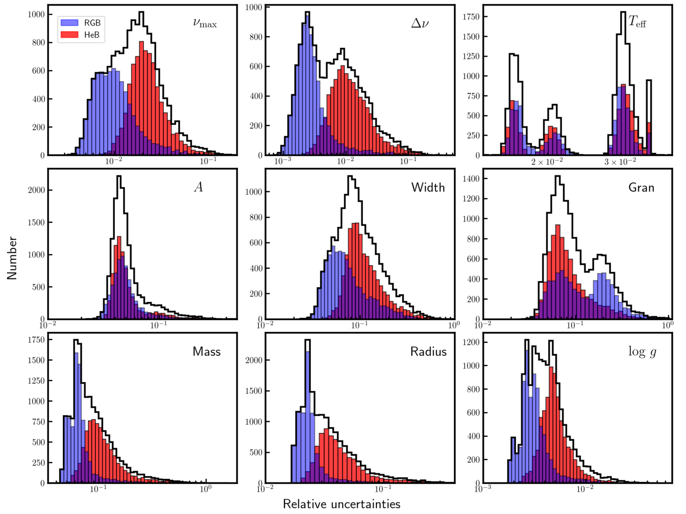
III.5 Uncertainties

The fractional uncertainties of seismic parameters and stellar fundamental properties are shown in Figure 6, based on full length end-of-mission long-cadence datasets. Considering output offset from different methods [52], we have added in quadrature 1.0% and 0.5% relative uncertainties in and to their formal uncertainties, respectively, only when deriving the uncertainties for mass, radius, and . The correction factor, , was fixed when determining the uncertainties of mass and radius using error propagation.
It can be seen from Figure 6 that and can be measured more precisely in RGB stars (blue) than in HeB stars (red). This is mainly because HeB stars generally exhibit more complicated power spectra. This effect is propagated into the estimates of mass, radius, and , which are derived from the scaling relations.
The effective temperatures from Mathur et al. [65] have four populations of distinct uncertainty distributions, from the KIC (Brown et al. 11, 4.0%), the DR24 stellar properties catalog (Huber et al. 51, 4.0%), the revised catalog of temperatures for long-cadence stars in the KIC (Pinsonneault et al. 80, 3.0%), and the high-resolution spectroscopy from APOGEE DR12 (Pinsonneault et al. 81, 2.0%, and Alam et al. 1, 1.7%).
The uncertainty of the granulation power for RGB stars is bimodal, with a significant peak at higher uncertainties, while the HeB has a similar distribution to the RGB at lower uncertainties. These features are a result of increasing fractional uncertainties of granulation power with and combined with the star number distribution as a function of of the entire sample. For the subsample with , we found that RGB and HeB stars have very similar and single-peaked fractional uncertainty distributions that peak just below 0.1. As increases, we see the right component gradually more clearly.
As expected, longer datasets enable us to determine global seismic parameters more precisely [42]. Thanks to the full-mission data sets used in our asteroseismic analysis (see Fig. 1), we report precise determinations of global seismic parameters and stellar fundamental properties, with typical (median) precisions of 1.6% in , 0.6% in , 4.7% in oscillation amplitude, 8.6% in granulation power, 8.8% in width of power excess, 7.8% in mass, 2.9% in radius, and 0.01 dex (or 0.4%) in . Considering only the 7839 stars with near full-mission data (time series longer than 1200 days), the uncertainty distributions shift slightly to lower values, while the overall distributions shapes look similar. The typical (median) fractional uncertainties are 1.4% in , 0.4% in , 4.6% in oscillation amplitude, 7.8% in granulation power, 7.9% in width of power excess, 6.9% in mass, 2.5% in radius, and 0.01 dex (or 0.3%) in . The seismic and non-seismic parameters and their uncertainties are given in Table 1 and 2.
III.6 Correlation between and
Figure 7 displays the well-established power-law relation between and [39, 89, 46]. The red dashed line shown in Figure 7a was fitted using an MCMC method and is expressed as , where , . As noted previously in the literature, the power law is unable to perfectly describe the relation between and , especially in the common parameter space of RGB and HeB stars [46]. We can also see a concentration of HeB stars constituting a hook originating from around , which we identify as the zero-age main-sequence for helium-core-burning.
In order to show this feature more clearly, we plotted as a function of in Figure 7b and 7c, color-coded by evolutionary phase and stellar mass, respectively. The ordinate, , has a mass dependence expressed as follows, by combining Equation 2 and 3:
| (7) |
Since red giants cover a relatively small range of effective temperature, there is a very minor effective temperature influence on the distribution in Figure 7b and 7c. A pronounced feature in Figure 7b is the distinct distributions of HeB and RGB stars. The HeB stars form a sharp hook-shaped structure originating from 30 Hz (low-mass stars) and extending to at 120 Hz (high-mass stars). Note that there exists a sharp and extremely well-defined edge related to red clump stars. This is likely associated with the fact that all stars below roughly 2 M☉ ignite helium in fully degenerate cores of very similar mass. This sharp edge also tells us that the scaling relations work well for the zero-age main-sequence of HeB stars.
In Figure 7c we note that some red clump stars have low-mass around or below 0.7 M☉. The lack of low-luminosity RGB stars ( 40 Hz) with such low-mass implies that there could be systematics in mass inferred with the scaling relations, or that at least some of those low-mass RGB stars undergo mass loss before reaching the HeB phase. Assuming the latter is the case, the slightly less sharp edge toward the lowest mass HeB stars, at roughly and , could be a sign of “chaotic” variation in mass loss. In addition, the lack of low-mass stars ( 0.7 M☉), marked by purple dots, at a higher regime ( 40 Hz) and the presence of the low-mass stars in the range 20 Hz, possibly suggest that the low mass stars with 20 Hz are in the AGB phase and have experienced mass loss.
III.7 Seismic H-R diagram

Figure 8 shows a seismic H-R diagram for the largest sample of Kepler solar-like oscillators so far, with being measured from this work for red giants, except for super-Nyquist red giants from Yu et al. [104], and from Huber et al. [46] for main-sequence and subgiant stars. We select rather than to illustrate the seismic H-R diagram, because can be more accurately measured for stars oscillating around the Nyquist frequency. Red giants oscillate with amplitudes ranging from a few tens to thousands of parts per million, as shown in the color. The characteristic oscillation timescales vary from hours up to days, as indicated by plotted on the right. A few outliers are present, mainly due to the poorly determined temperatures for those stars [65]. The large uncertainties of the temperatures blur the distributions of red clump stars, making it difficult to distinguish from RGB stars. We observe a sharp edge lying at ( ), corresponding to the upper limit of estimates in this work. Solar-like oscillations with greater than the long-cadence Nyquist frequency are generally detected with short-cadence data [33]. Murphy et al. [79] and Chaplin et al. [15], however, pointed out that it remains possible to detect these oscillation using long-cadence data. Yu et al. [104] subsequently identified 98 stars oscillating in the super-Nyquist frequency regime, up to 387 μHz. These super-Nyquist red giants are also plotted in Figure 8.

IV Mass and Metallicity effects on power excess parameters
IV.1 Power excess difference in RGB and HeB stars
Figure 9 shows that RGB and HeB stars follow different distributions of oscillation amplitude, granulation power, and the width of power excess (see Section III.4 for the evolutionary phase classification). The differences are negligible for low red clump stars ( Hz), but gradually become substantial for higher stars ( Hz), and significant for secondary clump stars (HeB stars that did not undergo a helium flash, due to the non-degenerate helium core). We confirm that secondary clump stars have lower oscillation amplitudes and granulation power, and broader power excesses compared to RGB stars at a given [72]. We have tested and found that the offsets of both oscillation amplitude and granulation power between RGB and clump stars, in the range , are mainly due to the difference in stellar mass between the two populations, followed by luminosity and temperature, using the formulas fitted by Huber et al. [46]. The oscillation amplitude and granulation power show tight correlations, and both increase when the star evolves up the RGB [59, 46, 57].


We checked whether the smoothing process is responsible for the broader power excesses of secondary clump stars. One might suspect that the broader power excess of a secondary clump star could artificially arise from the smoothing process applied to measure it. To test this, we selected 20 RGB and secondary clump stars, including stars with extreme width values, with the same values in the range and checked individual original power spectra without smoothing. We found the power excess of the secondary clump stars to be intrinsically broader than the RGB stars. Therefore, the difference of power excess width in Figure 9c is not a measurement bias. The broader power excess might reduce the precision when measuring , which will propagate into the seismic determinations of mass and radius.
The measured amplitude of dipole-mode suppressed RGB stars [88], as shown in Figure 9a, is smaller than that of normal RGB stars. This is a simple consequence of the lack of power in the dipole modes, which constitute about half the total power [88]. We find that the suppressed stars show 9% less granulation power than normal RGB stars, as shown in Figure 9b. This offset is presumably caused by the mass difference between the dipole-mode suppressed stars and the normal RGB stars. To understand this, we recall that (1) dipole-mode suppressed stars show a mass distribution shifted to larger masses compared to normal RGB stars [88, see Figure 10a, and Figure 2 in ]. (2) Granulation power is a decreasing function of stellar mass, as predicted by Kjeldsen & Bedding [59]. (3) The granulation power of dipole-mode suppressed stars follows the same relations as normal red giants [30].
IV.2 Mass effect
Many efforts have been made to investigate the dependence of oscillation amplitude and granulation power on stellar fundamental properties in field stars and open clusters [60, 59, 91, 46, 64, 72, 19, 57, 20, e.g., ]. The empirical relations as proposed by Kjeldsen et al. [60] and Kjeldsen & Bedding [59] predict that oscillation amplitude and granulation power depend on the luminosity, mass, and temperature. In this section we study the mass influence on oscillation and granulation using our sample of over 16,000 oscillating red giants.
As shown in Figure 10a, the oscillation amplitude is a decreasing function of , ranging from 600 ppm at 5 Hz down to 20 ppm at 200 Hz. We observe an extremely sharp upper boundary, which might be related to excitation and damping of oscillation modes. We note that there are a number of stars with low amplitudes along the bottom of the global trend. We have checked those stars and found that some have low S/N power spectra, with Kepler time series that are only a few quarters long. The low-amplitude stars could also be contaminated by nearby stars or diluted by their companions in binary systems [105, 83] or be exotic stars. Figure 10a also shows that high-mass HeB stars have overall lower amplitudes compared to RGB stars at a given . A clear mass gradient is present in RGB stars as well.
The granulation power determined at has a dependence on stellar mass, as shown in Figure 10b. Our results are in qualitative agreement with the predictions given by Kjeldsen & Bedding [59], where higher-mass stars are expected to have lower oscillation amplitude and granulation power [72].
Red giants show progressively narrower power excess when evolving toward the tip of the RGB. Only approximately three orders of modes can be detected in high-luminosity red giants with 5 Hz and seven orders of modes in low-luminosity red giants [93, 18]. We confirm that the width of power excess is an increasing function of stellar mass as shown in Figure 10(c) [72, see also]. Higher-mass stars with wider power excess and lower oscillation amplitude imply that the total oscillation power tends to be almost conserved among the stars of different mass [57].
As shown in Figure 10, granulation power correlates with oscillation amplitude. To see this more clearly, we plotted oscillation amplitude against granulation power in Figure 11a, color-coded by the evolutionary phase (RGB or HeB). The correlations are similar but distinct for RGB and HeB stars [57]. The two populations following different distributions are mainly caused by their different stellar fundamental properties: luminosity, mass, and temperature (thus radius and ), as we can see from Figures 11b-f. The temperature effect stands out among RGB stars but is not clear between RGB and HeB at a given oscillation amplitude, because of their similar temperatures. Our results are qualitatively consistent with the predictions by Kjeldsen & Bedding [59].
IV.3 Metallicity effect
Figure 12 shows the -amplitude relation color-coded by metallicity. We observe that in Figure 12a the metallicity effect is not visually striking, which is due to the fact that oscillation amplitudes have a stronger dependence on luminosity, mass, and temperature [59], blurring the possible metallicity influence. In this section we attempt to investigate the metallicity effect on oscillation and granulation. Instead of fitting to the luminosity and mass inferred from the scaling relations with possible systematics, we fit the oscillation amplitude as a function of the observables, , , and temperature, as
| (8) |
Here, is a scaling factor introduced so that our model does not have to pass through the solar reference point ( = 3.6 ppm). Equation 8 was converted to a logarithmic scale when implementing the fit. We attempted to study the metallicity influence on RGB and HeB stars separately, because the two populations have different distributions, as shown in Figure 9a and Figure 10a. In this work, metallicity estimates are adopted from Mathur et al. [65]. We excluded all the stars with 200 Hz because the backgrounds of their power spectra are hard to model due to the oscillations being close to the Nyquist frequency.

By removing the underlying contributions from luminosity, mass, and temperature [59], the significant metallicity influence stands out clearly, as shown in Figure 12b, where metal-rich stars oscillate with larger amplitudes than metal-poor stars. The fitted values and the corresponding uncertainties of the parameters are shown in Table 3. The fitted scaling factor differs from unity, consistent with the results by Corsaro et al. [20].
We repeated the fit on the HeB stars. The red clump and secondary clump stars in our sample differ significantly in metallicity. The former covers a much larger metallicity range than the latter, which are overall more metal rich. Considering our primary goal of investigating metallicity effects, we excluded secondary clump stars using a threshold . Figure 12d shows that the metallicity influence also exists for red clump stars, where metal-rich stars again oscillate with higher amplitudes at given , , and .
We note that the oscillation amplitudes of RGB and red clump stars have different levels of dependence on , , and temperature, as the two relations show in Figure 12. The influences of , , and temperature on RGB stars are more significant than those on red clump stars, as revealed by the globally larger absolute exponents of the relation for RGB stars versus those for red clump stars (see Table 3). The different influence is because the , , and temperatures of RGB stars vary more significantly than those for HeB stars.
| Parameters | phase | ||||
|---|---|---|---|---|---|
| Oscil. amp. | RGB | 2.020.02 | -2.850.04 | 2.950.05 | -1.820.05 |
| Red clump | 0.360.03 | -1.990.02 | 1.360.04 | -1.230.05 | |
| Gran. power | Red giants | 0.380.01 | -4.380.01 | 2.670.03 | -2.220.05 |
Notes: The fitted values and uncertainties of the parameters, namely , as defined in Equation 8. The oscillation amplitudes of RGB and red clump stars were fitted separately, while the granulation power of all red giants was fitted to the entire sample.
Since the intensity fluctuation caused by granulation is related to the contrast between dark and bright regions of granules, the opacity and limb-darkening should have a strong effect on granulation power. Thus, metallicity in turn might influence granulation power as well. Figure 13 displays the metallicity effect on granulation power measured at , using the same model as shown in Equation 8. From Figure 13a, we observe that the metallicity effect is visible in the range covered by secondary clump stars. With the attempt to remove underlying contributions from luminosity, mass, and temperature, Figure 13b indicates that the granulation power depends on metallicity, where metal-rich stars have larger granulation power than metal-poor stars.
Our results reveals that the effect of metallicity on the granulation power of field red giants are in agreement with the arguments given by Corsaro et al. [20], who found that metallicity causes a statistically significant variation in the amplitude of the granulation activity of stars in the open clusters NGC 6791, NGC 6819, and NGC 6811. Collet et al. [17] performed 3D hydrodynamical simulations of red giants with [Fe/H] from -3.0 through 0.0, and found that more metal-rich stars have larger granules (see their Figure 4) due to increased opacity. The increased horizontal size of a granule suggests metal-rich stars are expected to have greater granulation power, which is qualitatively consistent with our results. To understand this, we recall that a convection cell is usually assumed to travel a vertical distance proportional to the pressure scale height, , at a speed scaling with the sound speed, , thus the the characteristic timescale of a granule can be expressed as . The assumption of the horizontal size of a granule, , proportional to the pressure scale height yields . The proportionality of granulation power to , with being the rms intensity fluctuation and varying much less than , gives the granulation power , hence, larger granules are expected to have larger granulation power [59, 64, for more detail see].


To quantitatively measure the impact of metallicity on the oscillation amplitude and granulation power, we plot their residuals, in the sense of the observed divided by the fitted quantity, as a function of [Fe/H] in Figure 14. The magenta points are the mean values in each [Fe/H] bin with a width of 0.1 dex. A linear fit is also shown with the red line. Clearly, the oscillation amplitude depends on metallicity, causing a 15% variation across the metallicity range -0.7<[Fe/H] <0.5 for both RGB and red clump stars, and so does granulation power, but with a 25% scatter for the whole sample.
Note that when investigating the metallicity influence, we used [Fe/H] estimates from Mathur et al. [65], of which 48% originate from the KIC. Pinsonneault et al. [81] found that the KIC metallicities show good agreement with those from APOGEE for red giant stars (see their Figure 14). We also performed the same analysis but only using spectroscopic metallicity from Mathur et al. [65], and found that the metallicity influence remains significant, as shown in Figure 15.
V Conclusions and Discussions
We have presented a homogeneous analysis of 16094 oscillating red giants observed by Kepler mission using all available end-of-mission long-cadence data sets. We provide a catalog of global seismic parameters and seismically derived mass, radius, and therefore surface gravity for oscillators, with 5 Hz. We have also systematically investigated the distribution of oscillation amplitude, granulation power, and width of power excess in RGB and HeB stars separately, and their dependencies on stellar mass and metallicity. The main results are summarized as follows:
- •
We provide a catalog of seismic mass and radius and global oscillation parameters. The typical (median) uncertainties are 1.6% for , 0.6% for , 4.7% for oscillation amplitude, 8.6% for granulation power, 8.8% for width of power excess, 7.8% for mass, 2.9% for radius, and 0.01 dex for .
- •
We have improved the SYD pipeline to provide more accurate estimates, some of which were incorrectly measured to be . Our and measurements are in good agreement with the literature, displaying a median fractional residual of 0.2% and a scatter of 3.5% for , and a median fractional residual of 0.01% and a scatter of 4.2% for .
- •
We find that HeB stars form a extremely sharp edge, as shown in Fig 7b, which we interpret as the zero-age main-sequence for core helium-burning. We also find tentative evidence for mass loss at the RGB tip and AGB phase.
- •
RGB and HeB stars follow systematically different distributions of oscillation amplitude, power excess width, and granulation power. Secondary clump stars have an overall lower oscillation amplitude and granulation power, and broader power excess than RGB stars. This difference gradually attenuates toward lower- RGB and HeB stars.
- •
The oscillation amplitude and granulation power have dependencies on mass and metallicity. We confirm that the width of power excess is an increasing function of mass. Metallicity has an influence on oscillation amplitude, leading to 15% variation for RGB stars and red clump stars in the metallicity range , and on granulation power, causing a 25% spread for all the red giants in the sample. Metal-rich and lower-mass stars show larger oscillation amplitude and granulation power.
Given the difficulty of appropriately fitting the power spectrum background, we do not report the measurement of oscillation amplitude, width of power excess, or granulation power for stars with 200 Hz. We excluded all the stars with 275 Hz, though measurements of using an autocorrelation function method are less affected [104].
Recently, Mathur et al. [65] delivered a characterization of the stellar fundamental properties of Kepler targets for a transit detection run. This is based on conditioning stellar atmospheric parameters on the isochrones from the Dartmouth Stellar Evolution Database, which does not include helium-burning models for low-mass stars. Our seismic determinations of radius and mass are nearly independent of stellar models (except when correcting ) and therefore are able to remedy the bias of overestimated mass measurements for HeB stars.
Our asteroseismic stellar properties can be used as reliable distance indicators and age proxies for mapping and dating the Galactic disk, as observed by the Kepler telescope. It is also worthwhile to test and/or calibrate Gaia parallaxes. The precise and accurate seismically derived surface gravities lift the degeneracies from spectroscopically deriving atmospheric parameters. The and missions are not expected to perform seismology on stars that are as distant and faint as this sample, so these stars will remain benchmark red giants for many years to come.
Hon et al. [43] used our results for the successful classification of 5379 RGB and HeB stars. Wu et al. [102] deduced the ages of the RGB stars in our sample and applied them as a training data set to derive ages and masses directly from LAMOST spectra. Silva Aguirre et al. [86] chemically dissected the Milky Way disk population using a sample of red giant stars with the asteroseismic ages, which were determined using the global oscillation parameters measured from this work.
Our sample does not include stars oscillating with below 5 Hz. The scaling relations might not work appropriately because the low radial orders, n, of observed modes cannot be reliably approximated with an asymptotic theory. Thus, the seismically inferred stellar masses and radii would be biased. However, it is of significant interest to measure the pulsation amplitudes and periods of those late RGB and AGB stars observed by Kepler. This would be a great sample to investigate the correlation between the amplitude and period for long-period variables (LPVs, Mosser et al. [75], Stello et al. [93]) and their relation with mass loss (J. Yu et al. in prep.).
Acknowledgments
The authors would like to thank our anonymous referee for a careful reading of our manuscript and many helpful comments. We also want to thank Hans Kjeldsen for fruitful discussions. We gratefully acknowledge the entire Kepler team and everyone involved in the Kepler mission for making this paper possible. Funding for the Kepler Mission is provided by NASA’s Science Mission Directorate. Some/all of the data presented in this paper were obtained from the Mikulski Archive for Space Telescopes (MAST). STScI is operated by the Association of Universities for Research in Astronomy, Inc., under NASA contract NAS5-26555. Support for MAST for non-Hubble Space Telescope data is provided by the NASA Office of Space Science via grant NNX09AF08G and by other grants and contracts. D.H. acknowledges support by the Australian Research Council’s Discovery Projects funding scheme (project number DE140101364) and support by the National Aeronautics and Space Administration under Grant NNX14AB92G issued through the Kepler Participating Scientist Program. D.S. is the recipient of an Australian Research Council Future Fellowship (project number FT1400147).
References
- [1] Alam, S., Albareti, F. D., Allende Prieto, C., et al. 2015, ApJS, 219, 12
- [2] Bastien, F. A., Stassun, K. G., Basri, G., & Pepper, J. 2013, Nature, 500, 427
- [3] Batalha, N. M., Borucki, W. J., Koch, D. G., et al. 2010, ApJ, 713, L109
- [4] Beck, P. G., Montalban, J., Kallinger, T., et al. 2012, Nature, 481, 55
- [5] Bedding, T. R., Kjeldsen, H., Campante, T. L., et al. 2010, ApJ, 713, 935
- [6] Bedding, T. R., Mosser, B., Huber, D., et al. 2011, Nature, 471, 608
- [7] Belkacem, K., Goupil, M. J., Dupret, M. A., et al. 2011, A&A, 530, A142
- [8] Borucki, W. J., Koch, D., Basri, G., et al. 2010, Science, 327, 977
- [9] Brogaard, K., VandenBerg, D. A., Bruntt, H., et al. 2012, A&A, 543, A106
- [10] Brown, T. M., Gilliland, R. L., Noyes, R. W., & Ramsey, L. W. 1991, ApJ, 368, 599
- [11] Brown, T. M., Latham, D. W., Everett, M. E., & Esquerdo, G. A. 2011, AJ, 142, 112
- [12] Bruntt, H., Basu, S., Smalley, B., et al. 2012, MNRAS, 423, 122
- [13] Casagrande, L., Silva Aguirre, V., Schlesinger, K. J., et al. 2016, MNRAS, 455, 987
- [14] Cassisi, S., Castellani, V., Degl’Innocenti, S., Piotto, G., & Salaris, M. 2001, A&A, 366, 578
- [15] Chaplin, W. J., Elsworth, Y., Davies, G. R., et al. 2014a, MNRAS, 445, 946
- [16] Chaplin, W. J., Basu, S., Huber, D., et al. 2014b, ApJS, 210, 1
- [17] Collet, R., Asplund, M., & Trampedach, R. 2007, A&A, 469, 687
- [18] Corsaro, E., De Ridder, J., & García, R. A. 2015, A&A, 579, A83
- [19] Corsaro, E., Fröhlich, H.-E., Bonanno, A., et al. 2013, MNRAS, 430, 2313
- [20] Corsaro, E., Mathur, S., García, R. A., et al. 2017, A&A, 605, A3
- [21] De Ridder, J., Barban, C., Baudin, F., et al. 2009, Nature, 459, 398
- [22] Deheuvels, S., García, R. A., Chaplin, W. J., et al. 2012, ApJ, 756, 19
- [23] Deheuvels, S., Doğan, G., Goupil, M. J., et al. 2014, A&A, 564, A27
- [24] di Mauro, M. P., Cardini, D., Catanzaro, G., et al. 2011, MNRAS, 415, 3783
- [25] Di Mauro, M. P., Ventura, R., Cardini, D., et al. 2016, ApJ, 817, 65
- [26] Elsworth, Y., Hekker, S., Basu, S., & Davies, G. R. 2017, MNRAS, 466, 3344
- [27] Fröhlich, C., Andersen, B. N., Appourchaux, T., et al. 1997, Sol. Phys., 170, 1
- [28] Fuller, J., Cantiello, M., Stello, D., Garcia, R. A., & Bildsten, L. 2015, Science, 350, 423
- [29] García, R. A., Hekker, S., Stello, D., et al. 2011, MNRAS, 414, L6
- [30] García, R. A., Pérez Hernández, F., Benomar, O., et al. 2014, A&A, 563, A84
- [31] Gaulme, P., McKeever, J., Jackiewicz, J., et al. 2016, ApJ, 832, 121
- [32] Gilliland, R. L. 2008, AJ, 136, 566
- [33] Gilliland, R. L., Jenkins, J. M., Borucki, W. J., et al. 2010, ApJ, 713, L160
- [34] Gough, D. O. 1986, in Hydrodynamic and Magnetodynamic Problems in the Sun and Stars, ed. Y. Osaki (Uni. of Tokyo Press), 117
- [35] Guggenberger, E., Hekker, S., Angelou, G. C., Basu, S., & Bellinger, E. P. 2017, MNRAS, 470, 2069
- [36] Guggenberger, E., Hekker, S., Basu, S., & Bellinger, E. 2016, MNRAS, 460, 4277
- [37] Hekker, S., Elsworth, Y., Basu, S., et al. 2013a, MNRAS, 434, 1668
- [38] Hekker, S., Elsworth, Y., Mosser, B., et al. 2013b, A&A, 556, A59
- [39] Hekker, S., Kallinger, T., Baudin, F., et al. 2009, A&A, 506, 465
- [40] Hekker, S., Gilliland, R. L., Elsworth, Y., et al. 2011a, MNRAS, 414, 2594
- [41] Hekker, S., Elsworth, Y., De Ridder, J., et al. 2011b, A&A, 525, A131
- [42] Hekker, S., Elsworth, Y., Mosser, B., et al. 2012, A&A, 544, A90
- [43] Hon, M., Stello, D., & Yu, J. 2017, MNRAS, 469, 4578
- [44] Huber, D., Stello, D., Bedding, T. R., et al. 2009, Communications in Asteroseismology, 160, 74
- [45] Huber, D., Bedding, T. R., Stello, D., et al. 2010, ApJ, 723, 1607
- [46] —. 2011a, ApJ, 743, 143
- [47] Huber, D., Bedding, T. R., Arentoft, T., et al. 2011b, ApJ, 731, 94
- [48] Huber, D., Ireland, M. J., Bedding, T. R., et al. 2012, MNRAS, 423, L16
- [49] Huber, D., Carter, J. A., Barbieri, M., et al. 2013a, Science, 342, 331
- [50] Huber, D., Chaplin, W. J., Christensen-Dalsgaard, J., et al. 2013b, ApJ, 767, 127
- [51] Huber, D., Silva Aguirre, V., Matthews, J. M., et al. 2014, ApJS, 211, 2
- [52] Huber, D., Zinn, J., Bojsen-Hansen, M., et al. 2017, ApJ, 844, 102
- [53] Kallinger, T., Hekker, S., Garcia, R. A., Huber, D., & Matthews, J. M. 2016, Science Advances, 2, 1500654
- [54] Kallinger, T., Guenther, D. B., Matthews, J. M., et al. 2008, A&A, 478, 497
- [55] Kallinger, T., Weiss, W. W., Barban, C., et al. 2010a, A&A, 509, A77
- [56] Kallinger, T., Mosser, B., Hekker, S., et al. 2010b, A&A, 522, A1
- [57] Kallinger, T., De Ridder, J., Hekker, S., et al. 2014, A&A, 570, A41
- [58] Kjeldsen, H., & Bedding, T. R. 1995, A&A, 293, 87
- [59] —. 2011, A&A, 529, L8
- [60] Kjeldsen, H., Bedding, T. R., Arentoft, T., et al. 2008, ApJ, 682, 1370
- [61] Koch, D. G., Borucki, W. J., Basri, G., et al. 2010, ApJ, 713, L79
- [62] Li, T., Bedding, T. R., Huber, D., et al. 2018, MNRAS, 475, 981
- [63] Mathur, S., García, R. A., Huber, D., et al. 2016, ApJ, 827, 50
- [64] Mathur, S., Hekker, S., Trampedach, R., et al. 2011, ApJ, 741, 119
- [65] Mathur, S., Huber, D., Batalha, N. M., et al. 2017, ApJS, 229, 30
- [66] Michel, E., Baglin, A., Auvergne, M., et al. 2008, Science, 322, 558
- [67] Miglio, A. 2012, Astrophysics and Space Science Proceedings, 26, 11
- [68] Miglio, A., Brogaard, K., Stello, D., et al. 2012, MNRAS, 419, 2077
- [69] Miglio, A., Chiappini, C., Morel, T., et al. 2013, in European Physical Journal Web of Conferences, Vol. 43, European Physical Journal Web of Conferences, 3004, DOI: 10.1051/epjconf/20134303004
- [70] Mosser, B., Vrard, M., Belkacem, K., Deheuvels, S., & Goupil, M. J. 2015, A&A, 584, A50
- [71] Mosser, B., Belkacem, K., Goupil, M.-J., et al. 2010, A&A, 517, A22
- [72] Mosser, B., Elsworth, Y., Hekker, S., et al. 2012a, A&A, 537, A30
- [73] Mosser, B., Goupil, M. J., Belkacem, K., et al. 2012b, A&A, 548, A10
- [74] Mosser, B., Michel, E., Belkacem, K., et al. 2013a, A&A, 550, A126
- [75] Mosser, B., Dziembowski, W. A., Belkacem, K., et al. 2013b, A&A, 559, A137
- [76] Mosser, B., Benomar, O., Belkacem, K., et al. 2014, A&A, 572, L5
- [77] Mosser, B., Belkacem, K., Pinçon, C., et al. 2017, A&A, 598, A62
- [78] Murphy, S. J. 2012, MNRAS, 422, 665
- [79] Murphy, S. J., Shibahashi, H., & Kurtz, D. W. 2013, MNRAS, 430, 2986
- [80] Pinsonneault, M. H., An, D., Molenda-Żakowicz, J., et al. 2012, ApJS, 199, 30
- [81] Pinsonneault, M. H., Elsworth, Y., Epstein, C., et al. 2014, ApJS, 215, 19
- [82] Quinn, S. N., White, T. R., Latham, D. W., et al. 2015, ApJ, 803, 49
- [83] Schonhut-Stasik, J. S., Baranec, C., Huber, D., et al. 2017, ApJ, 847, 97
- [84] Sharma, S., Stello, D., Bland-Hawthorn, J., Huber, D., & Bedding, T. R. 2016, ApJ, 822, 15
- [85] Silva Aguirre, V., Casagrande, L., Basu, S., et al. 2012, ApJ, 757, 99
- [86] Silva Aguirre, V., Bojsen-Hansen, M., Slumstrup, D., et al. 2017, ArXiv e-prints, arXiv:1710.09847
- [87] Stello, D., Bruntt, H., Preston, H., & Buzasi, D. 2008, ApJ, 674, L53
- [88] Stello, D., Cantiello, M., Fuller, J., et al. 2016, Nature, 529, 364
- [89] Stello, D., Chaplin, W. J., Basu, S., Elsworth, Y., & Bedding, T. R. 2009, MNRAS, 400, L80
- [90] Stello, D., & Gilliland, R. L. 2009, ApJ, 700, 949
- [91] Stello, D., Huber, D., Kallinger, T., et al. 2011, ApJ, 737, L10
- [92] Stello, D., Huber, D., Bedding, T. R., et al. 2013, ApJ, 765, L41
- [93] Stello, D., Compton, D. L., Bedding, T. R., et al. 2014, ApJ, 788, L10
- [94] Stello, D., Huber, D., Sharma, S., et al. 2015, ApJ, 809, L3
- [95] Tassoul, M. 1980, ApJS, 43, 469
- [96] Ulrich, R. K. 1986, ApJ, 306, L37
- [97] Valenti, J. A., & Fischer, D. A. 2005, ApJS, 159, 141
- [98] Verner, G. A., Elsworth, Y., Chaplin, W. J., et al. 2011, MNRAS, 415, 3539
- [99] Vrard, M., Mosser, B., & Samadi, R. 2016, A&A, 588, A87
- [100] White, T. R., Bedding, T. R., Stello, D., et al. 2011, ApJ, 743, 161
- [101] White, T. R., Huber, D., Maestro, V., et al. 2013, MNRAS, 433, 1262
- [102] Wu, Y., Xiang, M., Bi, S., et al. 2017, ArXiv e-prints, arXiv:1712.09779
- [103] Yıldız, M., Çelik Orhan, Z., & Kayhan, C. 2016, MNRAS, 462, 1577
- [104] Yu, J., Huber, D., Bedding, T. R., et al. 2016, MNRAS, 463, 1297
- [105] Ziegler, C., Law, N. M., Morton, T., et al. 2017, AJ, 153, 66