Influence of multiplet structure on photoemission spectra of spin-orbit driven Mott insulators: application to
Abstract
Most of the low-energy effective descriptions of spin-orbit driven Mott insulators consider spin-orbit coupling (SOC) as a second-order perturbation to electron-electron interactions. However, when SOC is comparable to anisotropic Hund’s coupling, such as in Ir, the validity of this formally weak-SOC approach is not a priori known. Depending on the relative strength of SOC and anisotropic Hund’s coupling, different descriptions of the multiplet structure should be employed in the weak and strong SOC limits, viz. LS and jj coupling schemes, respectively. We investigate the implications of both the coupling schemes on the low-energy effective model and calculate the angle-resolved photoemission (ARPES) spectra using self-consistent Born approximation. In particular, we obtain the ARPES spectra of quasi-two-dimensional square-lattice Iridate in both weak and strong SOC limits. The differences in the limiting cases are understood in terms of the composition and relative energy splittings of the multiplet structure. Our results indicate that the LS coupling scheme yields better agreement with the experiment, thus providing an indirect evidence for the validity of LS coupling scheme for iridates. We also discuss the implications for other metal ions with strong SOC.
I Introduction
Competition between on-site spin-orbit coupling (SOC), Coulomb repulsion and crystal field interactions in Iridates gives rise to a plethora of unusual features. For one of the most studied iridium-based compounds, Sr2IrO4, localized transport [1, 2, 3], absence of metalization at high pressures [4, 5] and emergence of an odd-parity hidden order in Rh-doped Sr2IrO4 [6, 7] were observed experimentally but are still debated from a theoretical standpoint. On the other hand, despite many experimental indications of possible superconductivity in doped Sr2IrO4 – including observation of Fermi arcs and a -wave gap in electron-doped Sr2IrO4 [8, 9, 10] - no direct signatures of the superconducting state, such as zero electrical resistance and/or Meissner effect, have been observed in these systems yet.
The ground state of Sr2IrO4 is believed to be an antiferromagnet (AFM) of pseudospin . The experimental low-energy magnon dispersion is described well by the Heisenberg model with up to third neighbor.[11] On the theoretical side, such Heisenberg model is derived by projecting the superexchange Kugel-Khomskii model [12] onto the spin-orbit (SO) basis. [13] However, this is a valid approach only if the virtual intermediate doubly occupied states considered in the second order perturbation theory can be well approximated by the , , and basis set. Such a basis set is an eigenbasis of the full Coulomb Hamiltonian which includes the 10Dq crystal field as well as the Hund’s coupling, but not SOC. In other words, this approach is, strictly speaking, valid only in the limit of crystal field and Hund’s coupling much larger than SOC. In that case, the multiplet structure of configuration is well described by the LS coupling scheme. This is indeed the assumption made in many of the earlier works,[14, 15, 16, 17] for instance in 18 while deriving the t-J-like model of Sr2IrO4 to calculate the PES spectra. The PES spectra, thus obtained, reproduces the low-energy features of the experimental spectra remarkably well, which is both interesting and intriguing.
For materials with the large atomic number , such as Ir, SOC is expected to be large since it scales proportionally to . The SO splitting in the shell of transition metals is eV. In comparison, for transition metal (TM) atoms with partially filled shells, such as Fe, Ni and Co, it is one order of magnitude smaller ( eV). For such cases, LS coupling scheme describes the multiplet structure well.[19] For atoms with partially filled shells, such as Ru, Rh and Pd, the SO splitting is eV and there are increasing deviations from the LS coupling scheme.[19] For even heavier atoms, such as Bi and Pb, where SO splitting is eV, the LS coupling is expected to fail. In such cases, jj coupling scheme would be an appropriate choice to describe the multiplet structure.
Quantitatively, the relative strength of SOC and electron correlation is measured in terms of the ratio, [20]
| (1) |
where is the (single particle) on-site SOC strength and is a Slater integral connected to the Slater parameter as for configuration. [21] Using the Racah parameters cm-1 and cm-1 for Ir4+ ion[22] leads to . Substituting , we get
| (2) |
The LS coupling scheme is known to be a good approximation for . [20] Therefore, for the case of iridium the choice of the LS coupling scheme is questionable.
and TM oxides with ground state has attracted a lot of attention as it can lead to interesting effects such as excitonic magnetism in Van-Vleck type Mott Insulators [23] or even triplon condensation and triplet superconductivity.[24, 25, 26, 27] Here, caution must be exercised in the choice of the coupling scheme. For example, the authors of Ref. [26] claim that and transition metal ions with the configuration such as Re3+, Ru4+, Os4+ and Ir5+ realize a low-spin state because of relatively large Hund’s coupling and, therefore, the multiplet structure should be calculated within the LS coupling scheme. While this is likely to be true for Ru4+ as a -element, which is, in fact, the only element discussed in detail in Refs. [25, 26, 27], the validity of the statement for heavier transition metal ions with partially filled shell is not a priori known. In fact, recent analysis of resonant inelastic X-ray scattering data on double-perovskite iridium oxides with a formal valency of Ir5+ yields SOC strength eV and Hund’s coupling eV , suggesting jj coupling scheme to be appropriate for Ir5+. [28]
One of the most prominent differences in the weak and strong SOC strengths is the multiparticle multiplet structure which, in turn, affects the experimentally observed features such as the PES spectra. A clear understanding of how the low-energy description of SOC driven insulators modifies in the weak and strong SOC limits is fundamental in developing a satisfactory theoretical description for these systems.
In this article, therefore, we investigate the implication of the two coupling schemes in the effective low-energy description of the ARPES spectra. We discuss the multiplet structures of TM ions with the configuration in the weak and strong SOC limits, defined by the and coupling scheme, respectively. We, then, construct an effective low-energy - Hamiltonian used to describe the ARPES spectra. For brevity, we focus on to calculate the theoretical spectra within the Self Consistent Born Approximation (SCBA) in the jj coupling scheme and make explicit comparison with the corresponding results obtained earlier within the LS coupling scheme [18] as well as the experimental results. This is particularly relevant in view of the fact that, despite consensus, the validity of the LS coupling for has not been established. Also, a satisfactory theoretical description of is still being developed. [11, 29]
The present work provides an indirect evidence of the validity of the LS coupling scheme for . More importantly, we explicitly show the particular manifestation of the coupling schemes on the kinetic part of a generalized t-J-like Hamiltonian and discuss its ramifications. This further allows us to speculate and discuss other scenarios where such implications could be drastic.
This article is organized as follows. First, in Section II, we discuss the LS and the jj coupling schemes within the perturbation theory calculation of the multiplet structure. In particular, for the case of two holes on t2g shell relevant for theoretical modeling of the ARPES spectra of Iridates. In Section III, we discuss how the choice of the coupling scheme manifests itself in the t-J model. In Section IV, the relevance of all these results to the calculation of ARPES spectra on Sr2IrO4 will be discussed. Finally, we discuss some of the subtle issues and conclude in Sections V & VI, respectively.
II Coupling schemes
Calculating the ARPES spectral function for Sr2IrO4 amounts to calculating the Green’s function for the hole introduced into the AF ground state in the photoemission process. [18]
In the octahedral crystal field, the levels split into and manifolds. There are five electrons per Ir, so effectively there is one hole residing on the lower manifold. While the manifold is composed of , , and orbitals, the hole carries an effective orbital momentum and a spin due to orbital moment quenching. [30] Due to strong on-site SOC, the t2g levels further split into doublet and quartet and the hole occupies the lower energy doublet.[2, 13]
Adding a hole to the Ir4+ ion leads to the configuration. Since each hole has effective orbital momentum per hole, [30] the configuration effectively mimics the configuration and we focus on the multiplet structure of the latter. The multiplet structure depends on the coupling scheme, as shown in Fig. 1 and discussed in the following.
It is important to note that the need for considering either LS or jj coupling scheme arises only for the cases when there are more than one fermions per site. In such cases, the multi-particle multiplet structure differs in the weak and strong SOC limits. For undoped Sr2IrO4, with only one hole per site, both SOC and correlation effects can be treated on equal footing.[31, 32]
We begin with the full Hamiltonian of a system
| (3) |
Here, is the central field Hamiltonian and includes kinetic energy of all electrons, nucleus-electron Coulomb interaction and central-symmetric part of the Coulomb electron-electron repulsion:
| (4) |
where is the atomic number of the nucleus and is the total amount of electrons in the system. Residual Coulomb Hamiltonian describes the angular part of the Coulomb interaction between electrons:
| (5) |
and describes the sum of all the on-site spin-orbit interactions
| (6) |
Eq. (3) can be solved perturbatively, taking to be the unperturbed part of the Hamiltonian. The eigenstates of this unperturbed system are described by :
| (7) |
and define the electronic configuration where is a principal quantum number of the -th particle.
Relative strengths of and dictates the order of perturbation and leads to two different coupling schemes in the limiting cases. If , then the strongest perturbation to the eigenstates of can be calculated as . Electronic configurations then split into multiplet terms
| (8) |
characterized by the total orbital L and spin S momenta. SOC further splits these levels and each level is now described by the total momenta , as can be seen in Fig. 1.
On the other hand, the jj coupling scheme is applicable if , implying that is the strongest perturbation to . In practice, this means that L and S are not good quantum numbers anymore (i.e. they don’t even form good first order approximation to the (unknown) eigenbasis of the total Hamiltonian Eq. (3)) and the total J momentum has to be calculated as a sum of individual j momenta characterizing each particle.
In order to obtain the multiplet structure in the LS (jj) coupling scheme, an unambiguous link between the product states (for two holes) and the final multiplet set () should be established, where indicate the orbitals occupied by the holes, and . This is followed by another basis transformation to obtain the states in the total momenta. In the end, the correspondence between different J-states in the two coupling schemes can be obtained. This involves working with all possible configurations and could be tedious (for details, see Appendix A).
If, however, the multiplet structure in one of the coupling schemes is known, the multiplet structure in the other scheme can be obtained easily: the correspondence between the multiplets and obtained within the LS and jj coupling schemes can, in general, be described as [19]
| (9) |
Since the transition between LS and the jj coupling scheme is a change of the scheme of summation of four angular momenta, the transformation coefficients in (9) can be expressed in terms of symbols: [19]
| (10) | ||||
The values of the factor
are given, for example, in Table (5.23) of Ref. [19] or in Ref. [33].
Let us explicitly calculate how transforms into the .
| (17) |
Using table (5.23) of [19] we calculate the values of and arrive at
| (18) | |||||
On the other hand, composition of the state remains unchanged in the two coupling schemes. Similar to the states, there will also be a mixing between higher energy states, such as the two states, and . However, the mixing between states is omitted from Fig. 1 for clarity.
Using Eq. (9), it is, therefore, possible to obtain the relative composition of the multiplets in the different coupling schemes. This has interesting consequences for the low-energy effective Hamiltonian and the ARPES spectra. More importantly, this already provides an estimate of the relative redistribution of the spectral weight in the ARPES spectra.
III Manifestation of the coupling scheme in the model
Time evolution in the Green’s function of the hole introduced into Sr2IrO4 in the photoemission process is determined by the Hamiltonian
| (19) |
where is Heisenberg Hamiltonian describing the ground state of the system which depends on first-, second- and third- neighbor exchange parameters , and , describes the on-site energy of the triplet states, and represents the kinetic energy of the hole.[18]
As we are interested in the low-energy description, in the following, we will consider only the low energy sector of the multiplet structure consisting of and states. The states lie at much higher energies, approximately twice as large as the singlet-triplet splitting [32, 30], and are expected to have a small contribution to the low-energy model. We note, however, that the resulting reduced Hilbert space is not complete. As a result, a basis transformation between the product state basis and the multiplet basis (see Appendix A) in this reduced Hilbert space is not proper and leads to issues with normalization. Therefore, we consider the full set of 15 configurations (microstates) formed by two holes residing on the orbitals while deriving the correspondence between the multiplet structures in the two coupling schemes. The (physical) cutoff is to be imposed only after arriving at the final basis set which is a good approximation to the eigenstates of the full Hamiltonian.
Detailed knowledge of the multiplet composition in terms of the product states is also required for deriving the Hamiltonian. Therefore, in the following, we have used the explicit transformations in the jj coupling scheme, discussed in Appendix A.2 (Eq. (45) & (48)). Nevertheless, for completeness and for pedagogical reasons, we provide and discuss both the schemes in detail in Appendix A.
We consider the kinetic energy part of the effective model in the two coupling schemes. The derivation within the jj coupling scheme closely follows that in the LS coupling scheme[18] and consists of two main steps. We start with the application of basis transformations Eq. (45) & (48) to the hopping term of t-J model where is a general one-particle tight-binding (TB) Hamiltonian adopted from Ref. [18]. Subsequently, we apply the slave-fermion, Holstein-Primakoff, Fourier, and Bogoliubov transformations, leading to:
| (20) | ||||
where (h) represents the hole creation (annihilation) operator written in the low-energy multiplet basis comprising of singlet () and tripet states () with at spin-sublattices A and B:
| (21) |
/ represent the spin sublattice index accounting for the AF order and ()/() represents the magnon creation (annihilation) operator on the two sublattices.
For a realistic description of the motion of charge excitation in the AF background of pseudospins in Sr2IrO4, we consider tight binding parameters obtained from density functional theory [18] and exchange couplings up to third neighbor that fit the experimental magnon dispersion. Hopping parameters are described by matrices due to charge excitation’s internal degree of freedom and have been denoted by . The terms describe the nearest, next nearest, and third neighbor free hopping of the polaron (i.e. not coupled to magnons) and the vertices and describe the polaronic hopping. They are given by
| (22) |
for the free hopping matrix while the matrices containing vertices are
| (23) |
and
| (24) |
where -dependent hopping elements , , , and -, -dependent vertices , and are given in Appendix E.
Therefore, by means of Holstein-Primakoff transformation, we have effectively mapped the complicated many-body problem onto a simpler one, describing the motion of a polaronic quasiparticle composed of charge excitations dressed by the magnons. This is achieved by projecting out the interaction of magnons with each other as well as their renormalization by the quasiparticle propagator. These approximations comprise the well-known self-consisted Born approximation.[34, 35, 36, 37, 38, 39]

A schematic description of these steps and qualitative origin of terms is shown in Fig. 2. In the absence of SOC, the ground state consists of one hole per site, with a spin up or down and occupying one of the three degenerate orbitals, and a charge excitation composed of two holes (site , see Fig. 2(a)). The charge excitation is a many-body configuration , described by total spin and orbital moment . Wavefunction overlap between neighboring holes is material specific and can be obtained from density functional calculations.[18] In the presence of SOC (Fig. 2(b)), the ground state with one hole per site is an antiferromagnet of pseudospins. The excited state, previously described by and , must now be described using total momentum, connected to and using either LS or jj coupling scheme. Hopping parameters capture the motion of the charge excitations and their interaction with the magnons and are derived from ’s using basis transformations from LS and jj coupling schemes as discussed in see A.
Within SCBA (Fig. 2(c)), only the non-crossing diagrams for the fermion-magnon interaction are retained, leading to quasiparticle dressed with the magnon (polaron). The motion of the polaron is now described by the matrices which involves the coupling between the excitation and magnons and are derived from ’s by application of the slave-fermion, Holstein-Primakoff, Fourier, and Bogoliubov transformations (see App. B).
The structural similarity between the resulting Hamiltonians in the two coupling schemes (see Eq. (20) above and Eq. (68)) is evident. However, the W-terms describing the free and polaronic hoppings are different from the corresponding terms in the coupling scheme. Comparing Eqs (22 – 24) with Eqs. (69 – 71), one finds that changing the coupling scheme results in renormalization of free-polaron dispersion and vertices and , in particular for the matrix elements corresponding to the propagation of the polaron with a singlet character.
Thus, in the t-J model, the coupling scheme manifests itself in the following way: each term of kinetic Hamiltonian (20) containing () operator gets a renormalization factor of while those containing two of singlet creation (annihilation) operators get a factor of .
The above renormalization can be explained by the mixing of the two states, and , as one goes from the LS to the jj limit. This mixing is shown schematically in Fig. 1 with dotted lines. Therefore, although the choice of the coupling scheme can not result in the change of the number of multiplets or appearance of new multiplets, it can, however, have interesting consequences for the low-energy effective model.
As evident from Eq. (18), part of the spectral weight of configuration in LS coupling scheme is transferred to higher energies in jj coupling scheme, whereas some spectral weight from higher state is transferred to lower energies. In other words, the singlet state in the jj coupling scheme gets some admixture of previously excited states and only of the spectral weight of the singlet derived in the LS coupling scheme. This results in renormalization of the hopping amplitudes and vertices by a factor of , seen in Eqs. (22 – 24). The physical consequences of this renormalization will be discussed in the next section where the theoretical ARPES spectrum for Sr2IrO4 in both coupling schemes will be compared.
IV Influence of the coupling scheme on the spectral function of
Having obtained the vertices (Eqs. (22 – 24)) describing the propagation of the polaron in Sr2IrO4, we calculate the Green’s functions of the polaron and plot its spectral function whithin self consistent Born Approximation (SCBA).[18] Since we don’t know the exact value of splitting between and (see Fig. 1) which also depends on the Hund’s coupling , we consider as a free parameter and perform calculations for three values of such that the singlet-triplet splitting11 1 The factor of 5/8 originates from the fact that the (1/2, 3/2) state splits into a quintet () and a singlet (). takes values between and (see Fig. 3).

(a)

(b)

(c)

(d)

(e)
There are many recent ARPES experiments revealing the shape of the iridate spectral functions, [2, 43, 44, 45, 46, 47, 10, 48, 41] one of which [41] is shown on the Fig. 3. The salient features of the spectral function are (i) lowest-energy quasiparticle peak at (,) or (,)( point), followed by an energy gap of eV, (ii) well defined peak at (,) ( point), and (iii) a plateau around (,) ( point). While the qualitative features in all the experiments are same, there are some quantitative differences. For instance, the splitting between the peaks at the point and the point varies in the range eV — a feature crucial for explicit comparison with the experimental data.
Comparing Fig. 3 and Fig. 3, one can see that the low energy peaks at and points are present in the theoretical ARPES spectra obtained within both the coupling schemes. However, as opposed to the LS coupling scheme, for the jj coupling scheme, the peak at the point is significantly softened in the theoretical spectra. Furthermore, the energy gap between the peak positions at the point and the quasiparticle peak at is much larger for any value of singlet-triplet splitting.
(a)

(b)
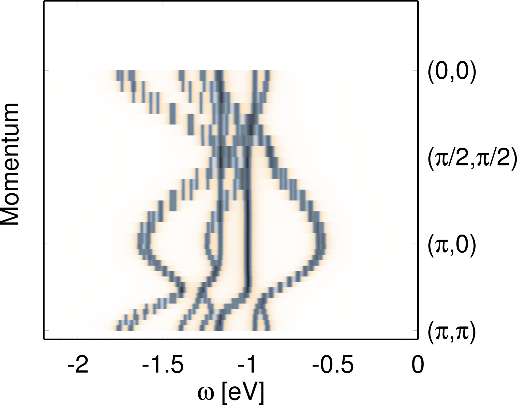
As Coulomb is varied, the most prominent change in the spectral function calculated within the jj coupling scheme is the change in the energy gap between the peak at the point and the quasiparticle peak. Although the size of this gap depends on the value of the singlet-triplet splitting, it is not fully determined by it. This shift of the quasiparticle peak is understood as an effect of the renormalization of the polaronic coupling discussed earlier. Relatively good qualitative and quantitative agreement with the experiment is obtained only with a small gap of (Fig. 3), which implies . However, as becomes comparable to , the LS coupling scheme should be used, which indeed shows a good qualitative and quantitative agreement with the experiments (Fig. 3).
It is interesting to note that in both LS and jj coupling schemes, there is a reasonably sharp peak at () as compared to a plateau in the experimental data. Although the peak at () is suppressed in the theoretical spectra too, owing to charge excitation scattering on magnons, clearly, this effect is not pronounced enough. This could arise due to overestimation of the quasiparticle spectral weight in SCBA. [34] Other possibilities include effects beyond the approximations made in the present study, such as hybridization of the TM orbitals with the O orbitals. Such effects are known to be important in cuprates where depending on the photon energy O or Cu weights are observed in the ARPES spectra. However, for quasi-2D iridium oxides, both ab-initio quantum chemistry calculation, as well as ARPES experiments, suggest that the charge gap is of the order of eV, while the Ir-O charge transfer gap is approximately 2-3 eV. [49, 50] Moreover, the charge gap in the iridates is believed to be a Mott-gap [51] that is much smaller than the charge transfer gap, putting the iridates in the Mott-Hubbard regime.
Yet another possibility is the role of higher lying states in the multiplet structure. However, since a realistic description of all the other low-energy features of the ARPES spectra is obtained for the singlet-triplet splitting or in the coupling scheme, the relative energy difference between the and the states is . Therefore, they are expected to have an insignificant contribution to the low-energy features. Nevertheless, such effects can not be ruled out completely.
Fig. 4 shows the relative contributions of the free and the polaronic part of the spectra in the jj coupling scheme for the singlet-triplet gap equal to . Comparison with the corresponding results in the LS coupling[18] indicates a stronger influence on the polaronic part of the spectra (Fig. 4) rather than on the free part (Fig. 4). Indeed, the hole of a singlet character has the largest contribution to the low-energy band (see Fig. 5) and when the strength of its coupling to magnons is increased by a factor of , the band gets additionally renormalized, thus indicating the importance of the polaronic processes.

(a)

(b)
V Discussions
Most of the SO driven strongly correlated materials lie in the intermediate spin-orbit coupling regime rather than in the extreme well defined by the LS or jj coupling schemes.[19] In fact, knowledge of the composition of the low-energy states and the relative energy splittings unambiguously dictates which coupling scheme is appropriate. In the absence of quantum chemistry results for Ir- configuration, one needs to resort to indirect verification of a suitable theoretical model.
For ions with intermediate SOC, ground state multiplets are in general much better captured by the LS coupling scheme than the excited states.[20] For example, even for some rare-earth compounds which have , LS coupling usually describes the experimentally measured lowest multiplet quite well, which is however not the case for higher excited states. For example, for Er+3 ion, which has a value of close to Ir, the ground-state wave function is given by [20]
| (25) |
i.e. the ground state is indeed well described by the LS coupling scheme. However, already for the highest exited multiplet in the same term we have
| (26) | ||||
We see that the multiplet , which according to the LS coupling scheme should describe , has in fact only % contribution in the corresponding excited wave function. [20]
It is also important to note that, in the case of Ir, the first excited state is not affected by the coupling scheme choice as there exist a unique state. However, this is not the case for, i.e., and configurations. In configuration, two lowest multiplets, and , can in general mix with each other as well as with higher lying . In the configuration, where the order of some states is inverted as compared to the configuration, the first two excited multiplets and do change places upon going from one coupling scheme to another,[19] probably rendering more pronounced effects in the theoretical description. One can, in general, expect much bigger ramifications of the coupling scheme choice in the cases where the composition of the excited states are different as well since under the same values of SOC they usually do get renormalized much more than the ground state, as exemplified by Eqs. (25) – (26).
Naturally, the same renormalization effect discussed in the present work would also be observed for an electron in the material with configuration in the ground state and strong on-site SOC for any geometry and choice of hopping parameters. For example, deriving a t-J model for a honeycomb iridates with one hole which forms the many-body configurations as well, one would get the same renormalization of the kinetic Hamiltonian when going from LS to jj limit, even though the motion of free charge on the honeycomb lattice is described by a completely different TB model: the hoppings between different orbitals are much larger than the hoppings between the same ones and they are moreover strongly bond-dependent.[52]
For the present case, employing the DFT-based TB parameters accounts for the crystal field effects and distortions such as octahedra rotation. We note, However, considerable differences from the present case are expected in strong distortions, e.g. under pressure, due to additional mixing of the states,[53] and, even more importantly, the renormalization of the Clebsch-Gordan coefficients.[13]
VI Conclusions
In conclusion, we have studied the ARPES spectra for quasi-2D square lattice iridates in weak and strong SOC strengths where the multiplet structures are well defined by different coupling schemes. Specifically, we have studied how the choice of the coupling scheme can influence the multiplet structure and consequently the low-energy effective model for , effectively described by configuration. We have shown that for a t-J-like model for Sr2IrO4, the jj coupling scheme induces renormalization of the vertices in the kinetic part of the Hamiltonian and prominent changes in the spectral function calculated within SCBA. We have compared the spectra calculated in both coupling schemes to the experimental ARPES data. Interestingly, despite large SOC, we find much better agreement to the experiment for the model derived within the LS coupling scheme. We argue that just as well as for many rare-earth compounds, which have comparable SOC strength, the spin-orbit coupling, albeit strong, is yet weak enough to allow for a successful description of the ground state in the framework of the LS coupling scheme.
For other electronic configurations, such as or , where all of the low-energy multiplets are renormalized as we go from LS to jj coupling scheme [54], more dramatic consequences are expected in the theoretical ARPES spectra.
Although, the choice of the coupling scheme and the effective low-energy model can be guided by the knowledge of the composition and relative energy splittings of the multiplets, in the absence of such experimental and/or quantum chemistry studies, the validity of the same must be ascertained.
VII Acknowledgements
Authors thank Manuel Richter, Klaus Koepernik, Krzysztof Wohlfeld, Jeroen van den Brink, Flavio Nogueira, Dmytro Inosov and Robert Eder for helpful suggestions and discussions. RR acknowledges financial support from the European Union (ERDF) and the Free State of Saxony via the ESF project 100231947 (Young Investigators Group Computer Simulations for Materials Design - CoSiMa.)
Appendix A Multiplet Structure
A.1 LS coupling scheme
To calculate the multiplet structure of configuration in LS coupling scheme as used in Ref. [18], one has to establish an unambiguous link between the single particle states (for two holes) and the final multiplet set where indicate the orbitals occupied by the holes, and . This is done in the following way.
First, one has to make a basis transformation from the real space basis to the single-particle states in the basis .[13] Secondly, for multi-particle configurations, one must construct the basis transformation from the product states to states described by total L and S. In principle, one can use Clebsch-Gordan coefficients (CGCs). However, there is a caveat: Clebsch-Gordan tables are formulated for summation of momenta of two inequivalent electrons. So, if we want to sum spins and of two electrons, they must be distinguishable. If they were on two different sites, then the position would suffice. However, if they are on the same site, as in our case, the multi-particle state can be obtained correctly by CGCs only if they reside on different orbitals. Bearing this in mind we avoid using CGCs for two-particle configurations and instead perform moment summation using the high weight decomposition method, discussed in detail in Appendix C.
As a result, we can construct the matrix that transforms the Hamiltonian from the product state basis to the total spin and orbital momentum basis :
| (27) |
where
and the product state basis is defined as
| (28) | |||||
where 1(0) represents the (un-)occupied single particle state of the Hilbert space spanned by . The multiplet basis is defined as
so that
| (30) |
Upon employing this transformation, we have effectively taken Hamiltonian (5) that defines the first-order corrections to the eigenstates of the system into account.
According to the Hund’s rules, the state with the lowest energy is the one with the highest multiplicity and the highest possible L, i.e. in the first approximation the ground state is the nine-fold degenerate multiplet.
To account for further perturbation on the system induced by the strong on-site spin-orbit coupling (Eq. (6)), we perform a basis transformation to obtain the total J momenta. To build a low-energy effective model, we truncate the Hilbert space down to the high spin states only. Since total spin and orbital momenta are distinguishable by their nature, we can simply use the CG coefficients to sum them up, leading to
| (31) |
where, is
is written in the spin-orbit coupled basis
| (41) |
which consists of the lowest singlet , the higher triplets (, split by energy from the singlet state) and quintets. [18]
To arrive at the final effective low-energy model we further truncate the Hilbert space and reduce the basis set to the two lowest multiplets and (see Fig 1):
| (42) |
A.2 jj coupling scheme
The jj coupling scheme is applicable if , implying that is the strongest perturbation to . In practice, this means that L and S are not good quantum numbers anymore (i.e. they do not even form a good first order approximation to the (unknown) eingenbasis of the total Hamiltonian Eq. (3)) and the total J momentum has to be calculated as a sum of individual j momenta characterizing each particle.
We now derive the basis transformation connecting Hamiltonian in the independent particle basis to the Hamiltonian defined in the basis of the total momenta J. In the jj coupling scheme, we first use CGCs to sum up the total momenta on each site
| (43) |
where the latter is written in the spin-orbit coupled single-particle basis . Since we perform CG summation here independently for both electrons, we have to take Pauli principle into account manually by projecting out forbidden states by hand. In the end, we arrive at:
| (44) | ||||
which is needed for
| (45) |
to transform the Hamiltonian from the basis (28) into the individual basis :
| (46) |
Now, we employ the high weight decomposition method to obtain Hamiltonian (Eq.(45)) in the total basis (see Appendix C.2 for details):
| (47) |
where is singlet state, represents a triplet state with , , signifies a quintet state with , and the superscript stands for . Basis (47) is equivalent to (41) when cut down to the lowest 9 states and to (42) upon further truncation to lowest 4 states.
In the end, we arrive at the final Hamiltonian
| (48) |
where, the basis transformation is
| (49) |
The correspondence between the two coupling schemes is obtained by matrix manipulation of the above matrices , , and , leading to results of Eq. (18).
Appendix B Derivation of W-terms
To illustrate the renormalization of different elements of W-terms, we consider a NNN hopping between the sites and which involves only hopping between orbitals at each site:
| (50) |
We transform this Hamiltonian into a basis that spans the full Hilbert space of two NNN sites . We do not explicitly show this transformed Hamiltonian here because of the size of the matrix (). The Hamiltonian in spin-orbit coupled basis within jj coupling scheme is then calculated as
| (51) |
where describes transformation of multiplet structure of a single hole/electron in three orbitals into total basis. This transformation is independent of the coupling scheme and can be obtained easily (see, e.g. 13, 31). Hamiltonian then produces another matrix with quite a few non-zero entries. For instance, the (1,12)-th matrix element is
| (52) |
where stands for creating an electron on site in the doublet with , and and , respectively, represent the creation of a charge excitation with singlet () and triplet (, ) character on site . The resulting Hamiltonian is then mapped onto a polaronic model as described in detail in e.g. Supplemental Material of 55. We subsequently introduce two antiferromagnetic sublattices and , and perform the Holstein-Primakoff transformation:
| (53) |
where stands for creating a magnon on sublattice A(B). Then, we translate it into space using Bogoluibov and Fourier transforms and obtain
| (54) |
Here, ()/ () represents the magnon creation (annihiliation) operator on the two sublattices A/B after the Bogoliubov transformation, and and are the Bogoliubov coefficients.[18] After this transformation has been performed for all the terms of Hamiltonian, the coefficients would enter the expressions.
Appendix C High weight decomposition method
C.1 LS coupling scheme
We start with the “high spin” state with the largest possible total spin and highest possible L for this S. Obviously, there are nine states with and which form the multiplet. From them we choose the one with the maximum projections and : . In terms of single-particle second quantization operators there is only one way this state can possibly be constructed:
| (56) |
where is an operator creating an electron on the orbital with and spin , and the vacuum state is defined as empty shell. To construct the next possible state we employ a ladder operator :
| (57) |
Using formula for the ladder operator known from textbooks (see for example Landau and Lifshitz [56])
| (58) |
and normalizing (57) we get
| (59) |
Now we can either apply once more or employ spin ladder operator instead. Let us look at the effect of the latter:
| (60) |
For a particular electronic configuration containing indistinguishable electrons according to the empirical Hund’s rule the ground state is the one with the largest possible for this configuration value of the total spin and the largest possible for this value of the total orbital momentum . So, having obtained all nine states of the multiplet in this way we proceed by searching for a state with the highest possible total orbital momentum. Since one has to place two electrons on the same orbital to get total orbital momentum , they must have opposite spins in order to obey Pauli’s principle. This state thus has , and belongs to quintet. Again, for the state with the highest possible momentum, be it orbital or spin, there is always one unique way to construct it:
| (61) |
It is important on this step to keep operator ordering convention consistent with that used in (56). After we have obtained all five states of multiplet using ladder operators, we only need to find the last missing state: singlet (full list of multiplets forming for a particular electronic configuration can be found in many atomic physics book, see e.g. Table 2.1 in [19]). We know that state shall have and , but we do not know what the quantum numbers , are. What we however know is that state has to be orthogonal to the other two states with and , which are written as
| (62) | ||||
Since there can be no other combination of two creation operators creating a state with both and other than the three used in (62) the missing state has to be a combination of them as well and simultaneously orthogonal to the two states in (62). Employing trivial linear algebra we get that the multiplet is written as
| (63) |
C.2 jj coupling scheme
We start from the state with highest possible . The state with the highest total momenta can be constructed either by placing one electron on the state with energy and one electron on the state or by placing two electrons on quartets both having energy so that a two-particle state has energy . Let us start with a state that is lower in energy
| (64) |
Applying ladder operator and normalizing the result we obtain the next state
| (65) | ||||
| (66) |
Once we have obtained five possible states we consider the other configuration formed by two electrons in the quartet:
| (67) |
Note that once chosen, the ordering convention has to be followed since fermionic operators anticommute.
Rest of the derivation is performed analogously to that in section C.1.
Appendix D model within the LS coupling scheme
The kinetic part of the in the coupling scheme is
| (68) | ||||
where the free hopping matrix is defined as
| (69) |
and the the matrices containing vertices are
| (70) |
| (71) |
Appendix E Free hopping and vertex elements
The nearest neighbor free hopping , and the polaronic diagonal and non-diagonal vertex elements are
| (72) | ||||
| (73) | ||||
| (74) | ||||
| (75) | ||||
| (76) | ||||
| (77) | ||||
| (78) | ||||
| (79) | ||||
| (80) | ||||
| (81) |
with and , where is the number of sites, and and are the Bogoliubov coefficients.[18]
The free hopping elements arising from the next-nearest and third neighbor hoppings are
| (82) | ||||
| (83) | ||||
| (84) | ||||
| (85) |
where . The polaronic next-nearest and third neighbor vertex elements are
| (86) | ||||
| (87) | ||||
| (88) | ||||
| (89) |
with .
References
- [1] J. Cheng, X. Sun, S. Liu, B. Li, H. Wang, P. Dong, Y. Wang, and W. Xu, New Journal of Physics 18, 093019 (2016).
- [2] B. J. Kim, H. Jin, S. J. Moon, J.-Y. Kim, B.-G. Park, C. S. Leem, J. Yu, T. W. Noh, C. Kim, S.-J. Oh, J.-H. Park, V. Durairaj, G. Cao, and E. Rotenberg, Phys. Rev. Lett. 101, 076402 (2008).
- [3] B. J. Kim, H. Ohsumi, T. Komesu, S. Sakai, T. Morita, H. Takagi, and T. Arima, Science 323, 1329 (2009).
- [4] D. Haskel, G. Fabbris, M. Zhernenkov, P. P. Kong, C. Q. Jin, G. Cao, and M. van Veenendaal, Phys. Rev. Lett. 109, 027204 (2012).
- [5] D. A. Zocco, J. J. Hamlin, B. D. White, B. J. Kim, J. R. Jeffries, S. T. Weir, Y. K. Vohra, J. W. Allen, and M. B. Maple, Journal of Physics: Condensed Matter 26, 255603 (2014).
- [6] L. Zhao, D. H. Torchinsky, H. Chu, V. Ivanov, R. Lifshitz, R. Flint, T. Qi, G. Cao, and D. Hsieh, Nat. Phys. 12, 32 (2016).
- [7] J. Jeong, Y. Sidis, A. Louat, V. Brouet, and P. Bourges, Nat. Commun. 8, 15119 (2017).
- [8] H. Wang, S.-L. Yu, and J.-X. Li, Phys. Rev. B 91, 165138 (2015a).
- [9] Y. K. Kim, O. Krupin, J. D. Denlinger, A. Bostwick, E. Rotenberg, Q. Zhao, J. F. Mitchell, J. W. Allen, and B. J. Kim, Science 345, 187 (2014a).
- [10] Y. K. Kim, N. H. Sung, J. D. Denlinger, and B. J. Kim, Nat. Phys. 12, 37 (2016).
- [11] J. Kim, D. Casa, M. H. Upton, T. Gog, Y.-J. Kim, J. F. Mitchell, M. van Veenendaal, M. Daghofer, J. van den Brink, G. Khaliullin, and B. J. Kim, Phys. Rev. Lett. 108, 177003 (2012).
- [12] A. M. Oleś, G. Khaliullin, P. Horsch, and L. F. Feiner, Phys. Rev. B 72, 214431 (2005).
- [13] G. Jackeli and G. Khaliullin, Phys. Rev. Lett 102, 017205 (2009).
- [14] O. N. Meetei, W. S. Cole, M. Randeria, and N. Trivedi, Phys. Rev. B 91, 054412 (2015).
- [15] T. Sato, T. Shirakawa, and S. Yunoki, Phys. Rev. B 91, 125122 (2015).
- [16] M. Kusch, V. M. Katukuri, N. A. Bogdanov, B. Büchner, T. Dey, D. V. Efremov, J. E. Hamann-Borrero, B. H. Kim, M. Krisch, A. Maljuk, M. M. Sala, S. Wurmehl, G. Aslan-Cansever, M. Sturza, L. Hozoi, J. van den Brink, and J. Geck, Phys. Rev. B 97, 064421 (2018).
- [17] Q. Chen, C. Svoboda, Q. Zheng, B. C. Sales, D. G. Mandrus, H. D. Zhou, J.-S. Zhou, D. McComb, M. Randeria, N. Trivedi, and J.-Q. Yan, Phys. Rev. B 96, 144423 (2017).
- [18] E. M. Pärschke, K. Wohlfeld, K. Foyevtsova, and J. van den Brink, Nat. Commun. 8, 686 (2017).
- [19] I. Sobelman, Atomic spectra and radiative transitions, 2nd ed. (Springer, 1996).
- [20] A. K. Zvezdin, V. M. Matveev, A. A. Mukhin, and A. I. Popov, Moscow Izdatel Nauka (1985).
- [21] G. Racah, Phys. Rev. 62, 438 (1942).
- [22] B. Andlauer, J. Schneider, and W. Tolksdorf, physica status solidi (b) 73, 533 (1976).
- [23] S. Agrestini, C.-Y. Kuo, K. Chen, Y. Utsumi, D. Mikhailova, A. Rogalev, F. Wilhelm, T. Förster, A. Matsumoto, T. Takayama, H. Takagi, M. W. Haverkort, Z. Hu, and L. H. Tjeng, ArXiv e-prints (2018), arXiv:1802.08752 [cond-mat.str-el] .
- [24] M. Horsdal, G. Khaliullin, T. Hyart, and B. Rosenow, Phys. Rev. B 93, 220502 (2016).
- [25] J. Chaloupka and G. Khaliullin, Phys. Rev. Lett. 116, 017203 (2016).
- [26] G. Khaliullin, Phys. Rev. Lett. 111, 197201 (2013).
- [27] A. Akbari and G. Khaliullin, Phys. Rev. B 90, 035137 (2014).
- [28] B. Yuan, J. P. Clancy, A. M. Cook, C. M. Thompson, J. Greedan, G. Cao, B. C. Jeon, T. W. Noh, M. H. Upton, D. Casa, T. Gog, A. Paramekanti, and Y.-J. Kim, Phys. Rev. B 95, 235114 (2017).
- [29] G. Cao and P. Schlottmann, Reports on Progress in Physics 81, 042502 (2018).
- [30] A. Abragam and B. Bleaney, Electron paramagnetic resonance of transitionions (Oxford University Press, 1970).
- [31] Z. Zhong, A. Tóth, and K. Held, Phys. Rev. B 87, 161102 (2013).
- [32] J. Griffith, The theory of transition-metal ions (Cambridge at the University Press, 1961).
- [33] H. Matsunobu and H. Takebe, Progress of theoretical physics 14, 589 (1955).
- [34] G. Martinez and P. Horsch, Phys. Rev. B 44, 317 (1991).
- [35] Z. Liu and E. Manousakis, Phys. Rev. B 45, 2425 (1992).
- [36] O. P. Sushkov, Phys. Rev. B 49, 1250 (1994).
- [37] J. van den Brink and O. P. Sushkov, Phys. Rev. B 57, 3518 (1998).
- [38] Y. Shibata, T. Tohyama, and S. Maekawa, Phys. Rev. B 59, 1840 (1999).
- [39] Y. Wang, K. Wohlfeld, B. Moritz, C. J. Jia, M. van Veenendaal, K. Wu, C.-C. Chen, and T. P. Devereaux, Phys. Rev. B 92, 075119 (2015b).
- [40] The factor of 5/8 originates from the fact that the (1/2, 3/2) state splits into a quintet () and a singlet ().
- [41] Y. Nie, P. King, C. Kim, M. Uchida, H. Wei, B. Faeth, J. Ruf, J. Ruff, L. Xie, C. Pan, X. amd Fennie, D. Schlom, and K. Shen, Phys. Rev. Lett. 114, 016401 (2015).
- [42] J. Kim, M. Daghofer, A. H. Said, T. Gog, J. van den Brink, G. Khaliullin, and B. J. Kim, Nat. Commun. 5, 5453 (2014b).
- [43] Q. Wang, Y. Cao, J. A. Waugh, S. R. Park, T. F. Qi, O. B. Korneta, G. Cao, and D. S. Dessau, Phys. Rev. B 87, 245109 (2013).
- [44] A. de la Torre, S. McKeown Walker, F. Y. Bruno, S. Riccó, Z. Wang, I. Gutierrez Lezama, G. Scheerer, G. Giriat, D. Jaccard, C. Berthod, T. K. Kim, M. Hoesch, E. C. Hunter, R. S. Perry, A. Tamai, and F. Baumberger, Phys. Rev. Lett. 115, 176402 (2015).
- [45] Y. Liu, L. Yu, X. Jia, J. Zhao, H. Weng, Y. Peng, C. Chen, Z. Xie, D. Mou, J. He, X. Liu, Y. Feng, H. Yi, L. Zhao, G. Liu, S. He, X. Dong, J. Zhang, Z. Xu, C. Chen, G. Cao, X. Dai, Z. Fang, and X. J. Zhou, Scientific Reports 5, 13036 (2015).
- [46] V. Brouet, J. Mansart, L. Perfetti, C. Piovera, I. Vobornik, P. Le Fèvre, F. m. c. Bertran, S. C. Riggs, M. C. Shapiro, P. Giraldo-Gallo, and I. R. Fisher, Phys. Rev. B 92, 081117 (2015).
- [47] Y. Cao, Q. Wang, J. A. Waugh, H. Reber, Theodore J.and Li, X. Zhou, S. Parham, N. C. Park, S.-R.and Plumb, E. Rotenberg, A. Bostwick, J. D. Denlinger, T. Qi, M. A. Hermele, G. Cao, and D. S. Dessau, Nature Communications 7, 11367 (2016).
- [48] A. Yamasaki, H. Fujiwara, S. Tachibana, D. Iwasaki, Y. Higashino, C. Yoshimi, K. Nakagawa, Y. Nakatani, K. Yamagami, H. Aratani, O. Kirilmaz, M. Sing, R. Claessen, H. Watanabe, T. Shirakawa, S. Yunoki, A. Naitoh, K. Takase, J. Matsuno, H. Takagi, A. Sekiyama, and Y. Saitoh, Phys. Rev. B 94, 115103 (2016).
- [49] V. M. Katukuri, H. Stoll, J. van den Brink, and L. Hozoi, Phys. Rev. B 85, 220402 (2012).
- [50] M. Uchida, Y. F. Nie, P. D. C. King, C. H. Kim, C. J. Fennie, D. G. Schlom, and K. M. Shen, Phys. Rev. B 90, 075142 (2014).
- [51] J.-M. Carter, V. Shankar, and H.-Y. Kee, Phys. Rev. B 88, 035111 (2013).
- [52] K. Foyevtsova, H. O. Jeschke, I. I. Mazin, D. I. Khomskii, and R. Valentí, Phys. Rev. B 88, 035107 (2013).
- [53] N. A. Bogdanov, V. M. Katukuri, J. Romhanyi, V. Yushankhai, V. Kataev, B. Buchner, J. van den Brink, and L. Hozoi, Nat. Commun. 6, 7306 (2015).
- [54] J. Rubio and J. J. Perez, Journal of Chemical Education 63, 476 (1986).
- [55] E. M. Plotnikova, M. Daghofer, J. van den Brink, and K. Wohlfeld, Phys. Rev. Lett. 116, 106401 (2016).
- [56] L. Landau and E. Lifshitz, Quantum mechanics: non-relativistic theory, 3rd ed. (Oxford: Pergamon Press, 1991).