Fast and rigorous arbitrary-precision computation of Gauss-Legendre quadrature nodes and weights
Abstract
We describe a strategy for rigorous arbitrary-precision evaluation of Legendre polynomials on the unit interval and its application in the generation of Gauss-Legendre quadrature rules. Our focus is on making the evaluation practical for a wide range of realistic parameters, corresponding to the requirements of numerical integration to an accuracy of about to bits. Our algorithm combines the summation by rectangular splitting of several types of expansions in terms of hypergeometric series with a fixed-point implementation of Bonnet’s three-term recurrence relation. We then compute rigorous enclosures of the Gauss-Legendre nodes and weights using the interval Newton method. We provide rigorous error bounds for all steps of the algorithm. The approach is validated by an implementation in the Arb library, which achieves order-of-magnitude speedups over previous code for computing Gauss-Legendre rules suitable for precisions in the thousands of bits.
keywords
Legendre polynomials, Gauss–Legendre quadrature, arbitrary-precision arithmetic, interval arithmeticAMS
65Y99, 65G99, 33C451 Introduction
The Legendre polynomials are the sequence of orthogonal polynomials with respect to the unit weight on the interval , normalized so that . Like other classical orthogonal polynomials, Legendre polynomials satisfy a three-term recurrence, in this case the relation
| (1) |
also known as Bonnet’s formula, and a second order differential equation, here
| (2) |
The definition implies that has roots all located in . Perhaps the most important application of Legendre polynomials is the Gauss-Legendre quadrature rule
| (3) |
where the nodes are the roots of . The quantity is called the weight associated with the node .
For some applications in computer algebra, number theory, mathematical physics, and experimental mathematics, it is necessary to compute integrals to an accuracy of hundreds of digits, and occasionally even tens of thousands of digits [2, 3, 9, 23]. The Gauss-Legendre formula eq. 3 achieves an accuracy of bits using evaluation points if is analytic on a neighborhood of , and if the neighborhood is large (that is, if the path of integration is well isolated from any singularities of ), then the constants hidden in the notation are close to the best achievable by any quadrature rule [22]. This quality is related to the fact that eq. 3 maximizes the order of accuracy among -point quadrature rules for integrating polynomials, being exact when is any polynomial of degree up to ; as a result, the accuracy is also excellent for analytic integrands that are well approximated by polynomials.11 1 However, statements about the near-optimality of Gauss-Legendre quadrature must not be over-interpreted. Indeed, the rate of convergence of Gauss-Legendre quadrature is not optimal asymptotically when for analytic on a fixed neighborhood, being improvable by a small factor [34].
In general, the error in eq. 3 can be bounded in terms of , or, if is analytic on an elliptical domain with foci at , in terms of and the semi-axes of the ellipse. Even when the conditions are not ideal for using eq. 3 directly, rapid convergence is often possible by combining eq. 3 with adaptive subdivision of the integration path [28]. We give some elements of comparison between Gauss-Legendre quadrature and alternative methods, such as Clenshaw-Curtis quadrature, in section 8.
The Gauss-Legendre scheme has the drawback that the quadrature nodes and weights are somewhat inconvenient to compute. Indeed, becomes highly oscillatory for large and hence presents difficulties for naive root-finding and polynomial evaluation methods. The classical Golub-Welsch algorithm avoids accuracy problems by formulating the task of computing the nodes as finding the eigenvalues of a tridiagonal matrix [13], but this approach is still too slow to be practical for large .
In the last decade, several authors have contributed to the development of asymptotic methods that permit computing any individual node and weight for arbitrarily large in time, culminating in the 2014 work by Bogaert [6, 15, 5]. For a review of this progress, see Townsend [32]. Of course, the ‘‘’’ bound assumes that a fixed level of precision is used. In the prevailing literature this generally means 53-bit IEEE 754 floating-point arithmetic. In addition, the available implementations rely in part on heuristic error estimates without rigorously proved bounds.
The literature on arbitrary precision or rigorous evaluation is comparatively limited. Petras [27] gave explicit bounds for the error when the roots of the Legendre polynomial are approximated using Newton iteration
| (4) |
provided that the initial values are computed by a certain asymptotic formula. However, Petras did not address the numerical evaluation of . Fousse [12] discussed the rigorous implementation of Gauss-Legendre quadrature using generic polynomial root isolation methods together with interval Newton iteration for root refinement, but did not study fast methods for large . Code for high-precision Gauss-Legendre quadrature rules can also be found in packages such as Pari/GP [31] and ARPREC [4], but without error analysis and without special techniques for large .
In the present article, we are interested in computing Gauss-Legendre nodes and weights to precisions significantly larger than machine precision—typically in the hundreds to thousands of bits—, with rigorous error bounds. As mentioned earlier, certain applications require enclosing the values of integrals to accuracies of this order, and it is often reasonable to use quadrature rules of degree that grows roughly linearly with for this purpose. For example, Johansson and Blagouchine [20] study the computation of Stieltjes constants to precisions of hundreds of digits using complex integration, building among other things on the work described in the present paper.
If we assume that the precision varies, basic arithmetic operations are no longer constant-time. It is well-known that addition, multiplication and division of -bit numbers (of bounded exponent) can be performed in operations [8], where the notation means that we neglect logarithmic factors. It is then clear that any node and weight can be computed to -bit accuracy in time, by performing Newton iterations eq. 4 from an appropriate initial value. As a consequence, the full set of nodes and weights for the degree- quadrature rule can be computed in time. For numerical integration of analytic functions where we typically have , a better (indeed, optimal) estimate than the classical bound is possible.
Theorem 1.
If for some fixed , then the Gauss-Legendre nodes and weights of degree can be computed to -bit accuracy in (equivalently, ) bit operations.
Proof sketch.
Using the formulae in [27], we can compute good initial values for Newton iteration in bit operations. The Newton iteration can be performed for all roots simultaneously using fast multipoint evaluation, which costs bit operations. Fast multipoint evaluation is numerically unstable and generically loses bits of accuracy, but we can compensate for this loss by using guard bits [21]. Since by assumption, this does not change the complexity bound.
Completing the details of the proof is a technical exercise. Despite being elegant in theory, the algorithm behind theorem 1 has a high overhead in practice, in large part due to the need to work with greatly increased precision. Working with expanded polynomials and processing all roots simultaneously also results in high memory usage and makes parallelization difficult. As discussed in section 5.2 below, an approach based on the ‘‘bit-burst’’ evaluation method for hypergeometric series leads to a similar complexity bound and may prove more practical for extremely large , but likely not for . We can achieve a slightly worse but still subcubic complexity of by employing fast multipoint evaluation in a completely different way to compute values in isolation [16], but unfortunately that algorithm also has high overhead.
In this work, we develop rigorous and more practical alternatives to the asymptotically fast algorithm outlined above. Our main contribution is to give a complete evaluation strategy for Legendre polynomials on in ball arithmetic [35, 19]. Computing the Gauss-Legendre nodes, then, is a relatively simple application of the results in [27] together with the interval Newton method [24]. For generating Gauss-Legendre quadrature rules with , our algorithm has an asymptotic bit complexity of like classical methods, but much lower overhead. For parameters which are most relevant to applications, the observed running time is effectively subcubic. Our algorithm outperforms that of theorem 1 for practically any combination of and in that range. Furthermore, if , the complexity reduces to as in the machine-precision implementations by Bogaert [5] and others.
The remainder of this paper is organized as follows. Section 2 gives an overview of our algorithm for evaluating Legendre polynomials. This is a hybrid algorithm that switches between different methods, detailed in the following sections, depending on the values of , , and . In section 3, we prove practical error bounds for the three-term recurrence eq. 1, which can be efficiently implemented in fixed-point arithmetic. This method is ideal for and up to a few hundred. For larger or , we use a fast method for evaluation of hypergeometric series. Section 4 discusses the hypergeometric series expansions that are preferable for different inputs and precision (including a well-known asymptotic expansion for large ), and section 5 their efficient evaluation. In section 6, we propose a strategy to select the best formula for any combination of . Section 7 presents benchmark results that compare the performance of our algorithm to some previous implementations as well as the asymptotically fast algorithm in theorem 1. Finally, section 8 reviews the viability of Gauss-Legendre quadrature compared to other methods for extremely high precision integration.
Our code for evaluating Legendre polynomials and computing Gauss-Legendre nodes and weights is freely available as part of the Arb library [19]22 2 http://arblib.org/.
2 General strategy
We work in the framework of midpoint-radius interval arithmetic, also called ball arithmetic [35, 19]. In general, given an integer and a ball , we want to evaluate at , yielding an enclosure such that holds for all .
We restrict our attention to real , which is the most interesting part of the domain for applications. Since , we can further restrict to . Bogaert [5] suggests working with instead of directly to improve numerical stability for close to . This is not necessary in arbitrary-precision arithmetic since a slight precision increase (of the order of bits, since the distance between two successive roots of close to is about ) works as well.
We note that, for rigorous evaluation of with complex as well as Legendre functions of non-integer order , generic methods for the hypergeometric function are applicable if is not extremely large; see [18]. Real can also be handled easily using naive methods.
In view of the use of Newton’s method to compute the roots, we also need to evaluate the derivative , typically at the same time as itself. A simple option is to deduce from and using
| (5) |
When is close to , though, this formula involves a cancellation of about bits in the subtraction, followed by a division by . Therefore, a direct evaluation of may be preferable to reduce the working precision. We use either of these strategies depending on the values of , , and .
Our evaluation algorithms rely on ball arithmetic internally to propagate the error bounds up to the final result. Therefore, to ensure that the enclosure output by our evaluation algorithm contains the image of the input, it is enough to have bounds on the truncation errors associated to each of the approximate expressions of that we use. The corresponding bounds are stated in equations eq. 19, eq. 26, and eq. 29.
To limit overestimation and computational overhead, we deviate from the direct use of ball arithmetic on two occasions. First, algorithm 1 does not keep track of round-off errors internally: instead, we prove an a priori bound on the accumulated error (corollary 6) and add it to the radius of the output ball after calling that algorithm. Second, since some methods would produce unsatisfactorily large enclosures when executed on input balls of radius , we evaluate (with higher internal precision if necessary) and and use a first-order bound
to separately bound the propagated error. Similarly, we use a bound for to compute a reasonably tight enclosure for . Suitable bounds are given in proposition 3. Denote by the coefficient of index in a power series , and write for two power series if has nonnegative coefficients and for all .
Lemma 2.
If , , , are such that and , then and .
Proposition 3.
The following bounds hold for :
| (6) | ||||
| (7) |
Proof.
It is classical that Legendre polynomials are given by the generating series
| (8) |
Differentiation with respect to yields
Set , so that the roots of are . Then, in the notation of lemma 2, we have the bound
In addition, Bernstein’s inequality for the Legendre polynomials [37] (see also [10]) combined with the logarithmic convexity of the Gamma function yields
and hence
By lemma 2, these bounds combine into
Since and using again the logarithmic convexity of , we conclude that
The result follows since all derivatives of Legendre polynomials reach their maximum at (or by using the bounds and lemma 2).
Remark 4.
By the same reasoning, the inequality
actually holds for all . Unfortunately, it seems to overestimate the envelope of by a factor about in the region where it is smaller than .
Based on these reductions, we assume from now on that is a floating-point number with . Our main algorithm for evaluating at combines the following methods:
- •
the iterative computation of via the three-term recurrence eq. 1,
- •
the asymptotic expansion eq. 17 of as ,
- •
- •
the analogous terminating expansion eq. 27 at .
All three expansions can be written as hypergeometric series, i.e., sums of the form where is a rational function of .
The constraints and heuristics used to select between these methods are described in detail below. Roughly speaking, the three-term recurrence is used for small index and precision , when is not too close to ; the asymptotic series when is large enough, again with not too close to ; the expansion at for large unless is close to ; and finally the expansion at in the remaining cases when is close to .
For an evaluation at -bit precision, we choose parameters such as truncation orders and internal working precision to target an absolute error of for some , corresponding to a relative error of about measured with respect to monotone envelopes for and as in [6]. The relative error of a computed ball for where is near a zero can be arbitrarily large, but the relative error of near will be small, which is sufficient for the Newton iteration method. Since the output consists of a ball, we also have the option of catching a result with large relative error and repeating the evaluation with a higher precision as needed.
3 Basecase recurrence
For small , a straightforward way to compute is to apply the three-term recurrence eq. 1, starting from and . Computing by this method takes about bit operations, where is the working precision and denotes the cost of -bit multiplication. It is thus attractive for small and , especially when both and are needed, since we can get at no additional cost.
Fix , and let . Bonnet’s formula eq. 1 gives
| (9) |
In a direct implementation of this recurrence in ball arithmetic, the width of the enclosures would roughly double at every iteration, requiring to increase the internal working precision by bits. We avoid this issue by performing an a priori round-off error analysis (to be presented now) of the evaluation that yields a less pessimistic bound on the accumulated error. Additionally, the static error bound allows us to implement the recurrence in fixed-point arithmetic, avoiding the overhead of floating-point and interval operations.
Suppose with is a given fixed-point number. Let denote the integer truncation of a real number (note that this is not the same thing as rounding to the nearest integer; however, any rounding function would do). The integer sequence defined by
| (10) |
is easy to compute using only integer arithmetic, and is an approximation of . Algorithm 1 provides a complete C implementation using GMP [14]. As a small optimization, we delay the division by until we have accumulated a denominator of the size of a machine word.
void legendre(mpz_t p, mpz_t q, int n, const mpz_t x, int t) {
mpz_t tmp; int k; mpz_init(tmp);
Comments use the notation of
mpz_set_ui(p, 1); mpz_mul_2exp(p, p, t);
mpz_set(q, x);
for (k = 1; k < n; k++) {
mpz_mul(tmp, q, x); mpz_tdiv_q_2exp(tmp, tmp, t);
mpz_mul_si(p, p, -k*k)
mpz_addmul_ui(p, tmp, 2*k+1);
mpz_swap(p, q);
if (mpn_mul_1(&denlo, &den, 1, k+1)) {
If multiplication overflows
mpz_tdiv_q_ui(p, p, den);
mpz_tdiv_q_ui(q, q, den);
den = k+1;
} else den = denlo;
}
mpz_tdiv_q_ui(p, p, den/n); mpz_tdiv_q_ui(q, q, den);
mpz_clear(tmp);
}
To bound the difference , we analyze the effect on the result of a small perturbation in each iteration of eq. 9. The bound is based on a classical linearity argument (compare, e.g., [36]) combined with majorant series techniques.
Proposition 5.
Suppose that a real sequence satisfies and
| (11) |
for arbitrary real numbers with for all . Then we have
for all .
Proof.
Let and . Subtracting eq. 9 from eq. 11 gives
| (12) |
with . Consider the formal generating series and . Noting that eq. 12 holds for all if the sequences and are extended by for and using the relations
we see that eq. 12 translates into
The solution of this differential equation with reads, cf. eq. 8,
This is an exact expression of the ‘‘global’’ error in terms of the ‘‘local’’ errors . Since and , it follows by lemma 2 that
and therefore
Corollary 6.
Suppose that for some and . The sequence defined by eq. 10 satisfies
| (13) |
Furthermore, the quantities , returned by algorithm 1 are such that
| (14) |
Proof.
We can write
for some , of absolute value at most one, and hence
where . proposition 5 applied to then provides the bound eq. 13.
Turning to algorithm 1, let , , denote the values of the variables , , before the loop, and , , their values at the end of iteration . Consider the sequence , , extended by and an arbitrary (finite) . For all , depending whether the conditional branch is taken, we have one of the systems of equations
| (15) | ||||||||
| (16) |
In both cases, we can write
with . The first equation implies for . Since the latter equality also holds for with , we can substitute it in the second equation, yielding
This relation holds for , and we extend it to by setting . Thus, also satisfies eq. 11 with , and proposition 5 applies. The final values of and are respectively and , whence the bound eq. 14.
We do not use asymptotically faster evaluation techniques for large in combination with this recurrence, since the series expansions to be presented next perform very well in this case.
4 Series expansions
For large or , we employ series expansions of with respect to either or rather than the algorithm from the previous section. The coefficients of the series are also computed by recurrence, but fewer than terms will typically be required. Let us now review the various series expansions that we are using (an asymptotic expansion as , series expansions at and ), before discussing their efficient evaluation in the next section.
4.1 Asymptotic series
For fixed or equivalently with , an asymptotic expansion for as can be given as [6, Eq. 3.4]
| (17) |
(for arbitrary ), where
| (18) |
and the error term satisfies
| (19) |
The coefficients are a hypergeometric sequence with
| (20) |
To evaluate the error bound, we can use the following inequality deduced from eq. 18:
| (21) |
The condition is satisfiable as soon as , as we can see by choosing and using the inequality . Since the Gauss-Legendre nodes are distributed linearly in , the asymptotic expansion gives a candidate algorithm for all but about of the nodes as . It is in fact a convergent series when , which allows evaluating to unbounded accuracy for fixed when . The particular form eq. 17 must be used for this purpose; there is a slightly different version of the expansion which is asymptotic to (for fixed when ) but paradoxically converges to (for fixed when ); see [25, Section 10.3] and [26, Section 18.15(iii)].
We can restate eq. 17 as a hypergeometric series by working with complex numbers. Letting , with and as usual, we have
and hence
| (22) |
This eliminates the explicit trigonometric functions and permits using algorithm 2 below to evaluate the series.
The evaluation of eq. 22 in ball arithmetic is numerically stable, and we therefore only need to add a few guard bits to the working precision.
4.2 Expansion at zero
If is even, the expansion of in the monomial basis reads
| (23) | ||||
and if is odd, we have
| (24) | ||||
where the hypergeometric sequences can be defined by and
| (25) |
At very high precision, we evaluate the full polynomials, where eq. 23 and eq. 24 have the advantage compared to other expansions of requiring only terms due to the odd-even form. At lower precision , the high order terms will be smaller than when is small, and we can truncate the series accordingly and add a bound for the omitted terms to the radius of the computed ball. When the series are truncated after the term (for any ), comparison with a geometric series shows that the error is bounded by the first omitted term times a simple factor.
Proposition 7.
For bounding in this expression, and for selecting an appropriate truncation point , we use the binomial closed forms eq. 23, eq. 24 together with the remarks in section 5.3.
The alternating series eq. 23 and eq. 24 may suffer from significant cancellation, which requires use of increased precision. We can estimate the magnitude by noting that no cancellation occurs if is an imaginary number. Solving the majorizing recurrence with , shows that
Therefore, the possible cancellation assuming that is about
bits (which is at most ), so using ball arithmetic with about bits of working precision for the series evaluation gives -bit accuracy.
4.3 Expansion at one
Expanding at yields
| (27) |
where . The coefficients are hypergeometric with initial value and term ratio
| (28) |
As in the previous section, we can truncate eq. 27 and bound the error by comparison with a geometric series.
Proposition 8.
For , eq. 27 does not suffer from cancellation. For , we can estimate the amount of cancellation from the magnitude of where . For not too large , a very good approximation is
We therefore need about bits of increased precision.
We can compute from and , but since this involves a division by , it is better to evaluate directly when is close to 1. We have where satisfies
| (30) |
Since , the analog
| (31) |
of proposition 8 holds with and as above.
5 Fast evaluation of series expansions
All these series expansions are amenable to fast evaluation techniques specific to multiple-precision arithmetic. Using such fast summation algorithms is critical for achieving good performance at high precision. We now discuss the algorithm that we use for evaluating the series of the previous section.
5.1 Rectangular splitting
We use rectangular splitting [29, 16] to evaluate hypergeometric series with rational parameters where the argument is a high-precision number. This reduces evaluating a -term series to cheap scalar operations (additions and multiplications or divisions by small integer coefficients) and about expensive nonscalar operations (general multiplications), whereas direct evaluation of the hypergeometric recurrence uses expensive operations.
Algorithm 2 presents our version of rectangular splitting for the present application. We implement the various series expansions by defining the functions used in steps 8 and 19 according to formulae eq. 20, eq. 25, eq. 28, eq. 30.
This algorithm is a generalization of the method for evaluating Taylor series of elementary functions given in [17], which combines rectangular splitting with partially unrolling the recurrence to reduce the number of scalar divisions (which in practice are more costly than scalar multiplications). The terms are computed in the reverse direction to allow using Horner’s rule for the outer multiplications.
Our code uses ball arithmetic for and so that no error analysis is needed, and we use a bignum type for (so no overflow can occur regardless of ). For low precision a faster implementation would be possible using fixed-point arithmetic with tight control of the word-level operations as was done for elementary functions in [17].
The algorithm contains two tuning parameters33 3 Let us stress that the choice of these parameters only affects the performance of the algorithm, not its correctness. The same remark holds every other time we resort to heuristics in this article.. The splitting parameter controls the number of multiplications for powers versus the number of multiplications for Horner’s rule. The choice is optimal, but when evaluating two series for the same (in our case, to compute both and ), the table of powers can be reused, and then minimizes the total cost.
The unrolling parameter controls the number of coefficients to collect on a single denominator, reducing the number of divisions to . Ideally, should be chosen so that and fit in 1 or 2 machine words. The example value is a reasonable default, but as an optimization, one might vary for each iteration of the main loop to ensure that always fits in a specific number of words.
The redundant parameter is a small convenience in the pseudocode. Setting and adding the constant term separately avoids having to make a special case to prevent division by zero when .
Due to the scalar operations, rectangular splitting ultimately requires arithmetic operations with bit complexity each just like straightforward evaluation of the recurrence, so it is not a genuine asymptotic improvement, but it is an improvement in practice and can give more than a factor 100 speedup at very high precision. It is possible to genuinely reduce the complexity of evaluating a hypergeometric sequence to arithmetic operations using a baby-step giant-step method that employs fast multipoint evaluation, but in practice rectangular splitting performs better until both and exceed (see [16]).
5.2 A note on the bit-burst method
Another technique for fast evaluation of hypergeometric series, called binary splitting, would be useful when is large and the argument is a rational number with small numerator and denominator, but this case is not relevant for our application. Binary splitting also forms the basis of the bit-burst method [11, Section 4], which permits evaluating any fixed hypergeometric series at any fixed point—without the restriction to simple rational numbers of plain binary splitting—to absolute precision in only bit operations. Yet, we do not use this method either in our implementation, due to its large overhead.
Indeed, computing by the bit-burst method method requires analytic continuation steps, each of which entails two evaluations of general solutions of the Legendre differential equation eq. 2. These solutions are defined by unit initial values at some intermediate point , and can be represented as a power series of radius of convergence whose coefficients obey recurrences of order two. This is to be compared with a single series, given by a first-order recurrence and typically converging faster, for the expansions considered in section 4.1 to section 4.3. Thus, the bit-burst method is unlikely to be competitive in the range of precision we are interested in, especially when the asymptotic series can be used.
Nevertheless, it can be shown that the solutions with unit initial values at of eq. 2 occuring at intermediate analytic continuation steps have Taylor coefficients at bounded by uniformly in and . As a consequence, the asymptotic cost of computing any individual root of by the bit-burst method and Newton iteration is . For computing all the roots, this approach matches the estimate of theorem 1, while allowing for parallelization and requiring less memory. It may hence provide an alternative to multipoint evaluation worth investigating for precisions in the millions of bits.
5.3 Binomial coefficients
The prefactors of both the series expansion at and the asymptotic series contain the central binomial coefficient . We need to compute this factor efficiently for any and precision . Since , it is best to use an exact algorithm when for some small constant . We use the binomial function provided by GMP for and otherwise use an asymptotic series for with error bounds given in [7, Corollaries 1 and 2].
We also need to quickly estimate the magnitude of binomial coefficients for error bounds of series truncations. We have the binary entropy estimate
and the equivalent form
| (32) |
The function can be evaluated cheaply with a precomputed lookup table. A coarse estimate is sufficient, since overestimating by a few percent only adds a few percent to the running time.
6 Algorithm selection
We first use a set of cutoffs found experimentally to decide whether to use the basecase recurrence or one of the series expansions. The recurrence is mainly faster for some combinations of , when computing simultaneously and for some combinations of , when computing alone (in all cases subject to some boundaries ); the actual optimal regions are complicated due to differences in overhead between fixed-point integer arithmetic and ball arithmetic for the respective algorithm implementations. For the actual cutoffs used, we refer to the source code.
To select between the series expansion at , the expansion at , and the asymptotic series, the following heuristic is used. For each algorithm , we estimate the evaluation cost as where is the number of terms required by algorithm ( if is the asymptotic series and it does not converge to the required accuracy), is the precision goal, and is the extra precision required by algorithm due to internal cancellation. For the asymptotic series, we multiply the cost by an extra factor 2 as a penalty for using complex numbers. In the end, we select the algorithm with the lowest .
We select and estimate heuristically using machine precision floating-point computations, working with logarithmic magnitudes to avoid underflow and overflow. For example, when is the asymptotic series, we search for a small such that for some small , in accordance with eq. 21. During the actual evaluation of the series expansions, and are then given; we compute rigorous upper bounds for the truncation error via eq. 19, eq. 21, eq. 26, eq. 29, eq. 31, eq. 32 using floating-point arithmetic with directed rounding, while additional rounding errors are tracked by the ball arithmetic.
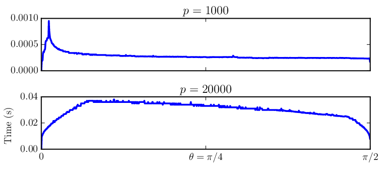
The assumption that the running time is a bilinear function of and is not completely realistic, but this cost estimate nonetheless captures the correct asymptotics when
separately, and hopefully will not be too inaccurate in the transition regions. This is verified empirically.
Figure 1 illustrates how the time to evaluate varies with when the automatic algorithm selection is used. Here, we have timed the case for two different . For large and (top plot), a sharp peak appears at the transition between the series expansion at and the asymptotic expansion which is used for most . This peak tends to become taller but narrower for larger . We could presumably get rid of the peak by implementing another algorithm specifically for the transition region, but the area under the peak is so small compared to the median baseline that computing all the roots would not be sped up much. For somewhat larger than (bottom plot), we observe a smooth transition between the series at near the left of the picture and the series at used over the most of the range.
7 Benchmarks
As already mentioned, our code for computing values and roots of Legendre polynomials is part of the Arb library, available from http://arblib.org/. The benchmark results given in this section were obtained using prerelease builds of version 2.13 of Arb. The implementation of the algorithms of this article is located in the files arb_hypgeom/legendre_p_ui_* of the Arb source tree. In section 7.1, we also use some ad hoc code available from this paper’s public git repository44 4 https://github.com/fredrik-johansson/legendrepaper/ when comparing the main algorithm with variants absent from the Arb implementation. The source code for the experiments themselves can be found in the same git repository. Except where otherwise noted, we ran the programs under 64-bit Linux on a laptop with a 1.90 GHz Intel Core i5-4300U CPU using a single core.
7.1 Polynomial evaluation
Figure 2 compares the performance of different methods for evaluating on a set of points distributed like the positive roots of to simulate one stage of Newton iteration at -bit precision. The time for the three-term recurrence is set to 1, i.e., we divide the other timings by this measurement. The following methods are timed:
- •
Our hybrid method (from here on called the ‘‘main algorithm’’) with automatic selection between the three-term recurrence and different series expansions.
- •
The main algorithm without the three-term recurrence as the basecase, i.e., using series expansions even for very small .
- •
Fast multipoint evaluation of the expanded polynomials and . As in section 4.2, we expand for even and for odd and evaluate at since this halves the amount of work. The polynomial coefficients are generated using the hypergeometric recurrence and the fast multipoint evaluation is done using _arb_poly_evaluate_vec_fast_precomp (where the ‘‘precomp’’ suffix indicates that the same product tree is used for both and ). The fast multipoint evaluation is done with guard bits, which was found experimentally to be sufficient for full accuracy.

The crossover point between the three-term recurrence and series expansions usually occurs around (it can be as low as if is much larger). For modest , the three-term recurrence is much faster than the hypergeometric series (typically by a factor 3-4) due to working with negligible extra precision and thanks to the low overhead of fixed-point arithmetic. This low overhead is very useful for typical evaluation of Legendre polynomials and generation of quadrature nodes for one or a few machine words of precision. The crossover point could be lowered slightly if we used a similarly optimized fixed-point implementation for the hypergeometric series.
When is fixed (top left in fig. 2), the main algorithm is a factor faster than the three-term recurrence since the asymptotic expansion converges to sufficient accuracy after terms for all sufficiently large . With the constant precision , the main algorithm is 3.0 times faster for and 30 times faster for . Conversely, fast multipoint evaluation with constant is a factor slower than our algorithm due to the higher internal precision.
When (the three remaining plots in fig. 2), the main algorithm appears to show the same speedup over the three-term recurrence after the crossover point, at least initially. This speedup should level off asymptotically, but in practice this only occurs for larger than where we have already gained a factor 10 or more. The leveling off is visible in the bottom right figure ().
Fast multipoint evaluation gives a true asymptotic speedup, but since it has much higher overhead, it only starts to give an improvement over the main algorithm from and for larger than . When , it appears that fast multipoint evaluation will only break even for much larger than . We conclude that fast multipoint evaluation would be worthwhile only for the last few Newton iterations when computing quadrature nodes for exceptionally high precision. Since independent evaluations are more convenient and easy to parallelize, the fast multipoint evaluation method currently seems to have limited practical value for this application.
7.2 Quadrature nodes
| 64 | 256 | 1 024 | 3 333 | 33 333 | |
|---|---|---|---|---|---|
| 20 | 0.000133 | 0.000229 | 0.000510 | 0.00121 | 0.0198 |
| 50 | 0.000450 | 0.000870 | 0.00212 | 0.00520 | 0.0710 |
| 100 | 0.00138 | 0.00310 | 0.00720 | 0.0163 | 0.191 |
| 200 | 0.00550 | 0.0111 | 0.0267 | 0.0550 | 0.589 |
| 500 | 0.0236 | 0.0610 | 0.164 | 0.325 | 2.61 |
| 1 000 | 0.0530 | 0.145 | 0.584 | 1.238 | 9.21 |
| 2 000 | 0.0860 | 0.298 | 1.12 | 4.20 | 32.6 |
| 5 000 | 0.191 | 0.665 | 2.67 | 14.3 | 181 |
| 10 000 | 0.350 | 1.26 | 4.93 | 26.6 | 674 |
| 100 000 | 3.60 | 12.2 | 41.3 | 212 | 13 637 |
| 1 000 000 | 58.0 | 146 | 411 | 1 850 | 103 960 |
| 64 | 256 | 1 024 | 3 333 | 33 333 | |
|---|---|---|---|---|---|
| 20 | 0.00059 () | 0.00070 () | 0.0015 () | 0.0035 () | 0.078 () |
| 50 | 0.0043 () | 0.0050 () | 0.010 () | 0.022 () | 0.43 () |
| 100 | 0.020 () | 0.023 () | 0.045 () | 0.089 () | 1.5 () |
| 200 | 0.11 () | 0.13 () | 0.24 () | 0.45 () | 6.5 () |
| 500 | 2.0 () | 2.1 () | 2.9 () | 5.1 () | 58 () |
| 1 000 | 25 () | 26 () | 29 () | 39 () | 300 () |
| 2 000 | 496 () | 478 () | 474 () | 532 () | 1 880 () |
The function arb_hypgeom_legendre_p_ui_root(x, w, n, k, p) sets the output variable to a ball containing the root of with index (we use the indexing , with giving the root closest to 1), computed to -bit precision. It also sets to the corresponding quadrature weight. We use the formulae in [27, Theorem 1(c)] to compute an initial enclosure with roughly machine precision, followed by refinements with the interval Newton method at doubling precision steps for very high precision. We deduce the quadrature weights thanks to the classical expression as functions of the nodes recalled in equation eq. 3.
Table 1 shows timings for computing degree- Gauss-Legendre rules to -bit precision by calling this function repeatedly with . Table 2 compares our code to the intnumgaussinit function in Pari/GP which uses a generic polynomial root isolation strategy followed by Newton iteration for high precision refinement. The improvement is most dramatic for small and large where we benefit from using asymptotic expansions, but we also obtain a consistent speedup for large .
For low precision and large , our implementation is about three orders of magnitude slower than the machine precision code by Bogaert [5] which is reported to compute the nodes and weights for in 0.02 seconds on four cores. This difference is reasonable since we use arbitrary-precision arithmetic, compute rigorous error bounds, and evaluate the Legendre polynomials explicitly whereas Bogaert uses a more sophisticated asymptotic development for both the nodes and the weights.
We also note that we can compute 53-bit floating-point values with provably correct rounding in about the same time as the 64-bit values, using Ziv’s strategy of increasing the precision. For a ball with relative radius just larger than , there is less than a probability that the correct 53-bit rounding cannot be determined, in which case that particular node can be recomputed with a few more bits.
Fousse [12] reports a few timings for smaller and high precision obtained on a 2.40 GHz AMD Opteron 250 CPU. For example, takes 0.14 seconds (our implementation takes 0.029 seconds) and takes 17 seconds (our implementation takes 0.53 seconds). Of course, these timings are not directly comparable since different CPUs were used.
The mathinit program included with version 2.2.19 of D. H. Bailey’s ARPREC library generates Gauss-Legendre quadrature nodes using Newton iteration together with the three-term recurrence for evaluating Legendre polynomials [4, 2]. With default parameters, this program computes the rules of degree for at 3 408 bits of precision, intended as a precomputation for performing degree-adaptive numerical integrations with up to 1 000 decimal digit accuracy. This takes about 1 300 seconds in total (our implementation takes 32 seconds). A breakdown for each degree level is shown in table 3.
Table 3 also shows the approximation error and the evaluation time (not counting the computation of the nodes and weights) for the degree- approximations of three different integrals, illustrating the relative costs and realistic requirements for . As motivation for the third integral, we might think of a segment of a Mellin-Barnes integral. The log, Airy and gamma function implementations in Arb are used.
| ARPREC | Our code | |||||||
|---|---|---|---|---|---|---|---|---|
| Error | Time | Error | Time | Error | Time | |||
| 12 | 0.00520 | 0.000592 | ||||||
| 24 | 0.0189 | 0.00171 | ||||||
| 48 | 0.0629 | 0.00507 | ||||||
| 96 | 0.251 | 0.0163 | ||||||
| 192 | 0.974 | 0.0532 | 0.075 | |||||
| 384 | 3.83 | 0.195 | 0.023 | 0.15 | 1.3 | |||
| 768 | 15.2 | 0.763 | 0.045 | 0.29 | 2.5 | |||
| 1 536 | 60.9 | 2.82 | 0.091 | 5.0 | ||||
| 3 072 | 241 | 9.55 | ||||||
| 6 144 | 1 013 | 18.3 | ||||||
| Time | ||||||||
|---|---|---|---|---|---|---|---|---|
| Error | Time | Error | Time | Error | Time | |||
| 1 989 | 0.12 | 0.93 | 6.3 | |||||
| 3 977 | 0.25 | 1.75 | 13.0 | |||||
| 7 955 | 0.55 | 3.49 | 25.1 | |||||
The last few degree levels (with roughly larger than the number of decimal digits) used by ARPREC tend to be dispensable for well-behaved integrands. A larger is needed if the path of integration is close to a singularity or if the integrand is highly oscillatory. In such cases, bisecting the interval a few times to reduce the necessary is often a better tradeoff. On the other hand, since the time to generate nodes with our code only grows linearly with beyond , increasing the degree further is viable, and potentially useful if the integrand is expensive to evaluate.
In the present work, we refrain from a more detailed discussion of adaptive integration strategies and the computation of error bounds for the integral itself. However, we mention that Arb contains an implementation of a version of the Petras algorithm [28] for rigorous integration. This code uses both adaptive path subdivision and Gauss-Legendre quadrature with an adaptive choice of up to by default, with degree increments and automatic caching of the nodes for fast repeated integrations. Node generation takes at most a few seconds for a first integration at 1 000-digit precision and a few milliseconds for 100-digit precision.
8 Gauss-Legendre versus Clenshaw-Curtis and the double exponential method
The Clenshaw-Curtis and double exponential (tanh-sinh) quadrature schemes have received much attention as alternatives to Gauss-Legendre quadrature for numerical integration with very high precision [30, 2, 33]. Both schemes typically require a constant factor more evaluation points than Gauss-Legendre rules for equivalent accuracy, but the nodes and weights are easier to compute. Gauss-Legendre quadrature is therefore the best choice when the integrand is expensive to evaluate or when nodes can be precomputed for several integrations. It is of some interest to compare the relative costs empirically.
Here we assume an analytic integrand with singularities well isolated from the finite path of integration so that Gauss-Legendre quadrature is a good choice to begin with. As observed in [33], Clenshaw-Curtis often converges with identical rate to Gauss-Legendre for less well-behaved integrands, and the double exponential method is far superior to either Clenshaw-Curtis or Gauss-Legendre for analytic integrands with endpoint singularities.
Clenshaw-Curtis quadrature uses the Chebyshev nodes , and the corresponding weights can be expressed by a discrete cosine transform which takes arithmetic operations to compute by an FFT. As a rule of thumb, -point Clenshaw-Curtis quadrature gives the same accuracy as -point Gauss-Legendre quadrature (for instance, the 384-point Clenshaw-Curtis rule gives errors of , and for the three integrals in table 3). As a point of comparison with tables 1 and 3, Arb computes a length-2 048 FFT with 1 000-digit precision in 0.09 seconds and a length-32 768 FFT with 10 000-digit precision in 36 seconds. The precomputation for Clenshaw-Curtis quadrature is therefore roughly a factor 20 cheaper than for Gauss-Legendre quadrature with our algorithm, while subsequent integration with cached weights is twice as expensive for Clenshaw-Curtis.
Double exponential quadrature uses the change of variables to convert an integral on to the interval in such a way that the trapezoidal rule converges exponentially fast. One generally chooses the discretization parameter as so that both the evaluation points and weights can be recycled for successive levels , and is chosen so that the tail of the infinite series is smaller than . The nodes and weights can be computed with exponential function evaluations and arithmetic operations. Double exponential quadrature with evaluation points typically achieves the same accuracy as -point Gauss-Legendre quadrature, where is slightly larger than for Clenshaw-Curtis, e.g. ; see table 4. The time to compute nodes and weights is comparable to Clenshaw-Curtis quadrature (around 0.2 seconds for 1 000-digit precision and two minutes for 10 000-digit precision).
In summary, for integration with precision in the neighborhood of to digits, computing nodes with our algorithm is about an order of magnitude more expensive than performing elementary function (e.g. exp or log) evaluations or computing an FFT of length . This makes Gauss-Legendre quadrature competitive for computing more than integrals (assuming that nodes and weights are cached), for a single integral requiring splitting into subintervals, or for a single integral when the integrand costs more than elementary function evaluations, where .
The picture becomes more complicated when accounting for the method used to estimate errors in an adaptive integration algorithm. One drawback of the Gauss-Legendre scheme is that the nodes are not nested, so that an adaptive strategy that repeatedly doubles the quadrature degree requires twice as many function evaluations as the degree of the final level. This drawback disappears if the error is estimated by extrapolation or if an error bound is computed a priori as in the Petras algorithm [28].
9 Conclusion
In [2], it was claimed that ‘‘There is no known scheme for generating Gaussian abscissa–weight pairs that avoids [the] quadratic dependence on . High-precision abscissas and weights, once computed, may be stored for future use. But for truly extreme-precision calculations – i.e., several thousand digits or more – the cost of computing them even once becomes prohibitive’’.
In this quote, ‘‘quadratic dependence’’ refers to the number of arithmetic operations. We may remark that using asymptotic expansions in the evaluation of Legendre polynomials avoids the quadratic dependence on for fixed precision , and theorem 1 avoids the implied cubic time dependence on when . In fact, theorem 1 implies that Gauss-Legendre, Clenshaw-Curtis and double exponential quadrature have the same quasi-optimal asymptotic bit complexity, up to logarithmic factors.
Our experiments show that the algorithm in theorem 1 hardly is worthwhile. However, the hybrid method described in sections 2 to 5 does achieve a significant speedup for practical and which allows us to compute Gauss-Legendre quadrature rules for 1 000-digit integration in 1-2 seconds and for 10 000-digit integration in 10-20 minutes on a single core. This is not prohibitively expensive compared to the repeated evaluation of typical integrands, especially if several integrations are needed. Parallelization is also trivial since all roots are computed independently.
A natural extension of this work would be to consider Gaussian quadrature rules for different weight functions. The techniques should transfer to other classical orthogonal polynomials (Jacobi, Hermite, Laguerre, etc.) which likewise have hypergeometric expansions and satisfy three-term recurrence relations. The main obstacle might be to obtain large- asymptotic expansions with suitable error bounds.
Acknowledgements
We are indebted to Nick Trefethen and two anonymous referees for their useful comments. We also thank Bruno Salvy for pointing out Petras’ paper [27]. Marc Mezzarobba was supported in part by ANR grant ANR-14-CE25-0018-01 (FastRelax).
References
- [1] V. Antonov and K. Holševnikov, An estimate of the remainder in the expansion of the generating function for the Legendre polynomials (generalization and improvement of Bernstein’s inequality), Vestnik Leningrad Univ. Mat., 13 (1981), pp. 163–166. English translation of [37] by H. H. McFadden.
- [2] D. H. Bailey and J. M. Borwein, High-precision numerical integration: Progress and challenges, J. Symbolic Comput., 46 (2011), pp. 741–754, http://dx.doi.org/10.1016/j.jsc.2010.08.010.
- [3] D. H. Bailey, J. M. Borwein, and R. E. Crandall, Integrals of the Ising class, J. Phys. A, 39 (2006), p. 12271, http://dx.doi.org/10.1088/0305-4470/39/40/001.
- [4] D. H. Bailey, H. Yozo, X. S. Li, and B. Thompson, ARPREC: An arbitrary precision computation package, 2002.
- [5] I. Bogaert, Iteration-free computation of Gauss–Legendre quadrature nodes and weights, SIAM J. Sci. Comput., 36 (2014), pp. A1008–A1026, http://dx.doi.org/10.1137/140954969.
- [6] I. Bogaert, B. Michiels, and J. Fostier, O(1) computation of Legendre polynomials and Gauss–Legendre nodes and weights for parallel computing, SIAM J. Sci. Comput., 34 (2012), pp. C83–C101, http://dx.doi.org/10.1137/110855442.
- [7] R. P. Brent, Asymptotic approximation of central binomial coefficients with rigorous error bounds, 2016, http://arxiv.org/abs/1608.04834.
- [8] R. P. Brent and P. Zimmermann, Modern Computer Arithmetic, Cambridge University Press, 2010, http://www.loria.fr/~zimmerma/mca/mca-cup-0.5.7.pdf.
- [9] D. Broadhurst, Feynman integrals, L-series and Kloosterman moments, Feb. 2016, http://arxiv.org/abs/1604.03057.
- [10] Y. Chow, L. Gatteschi, and R. Wong, A Bernstein-type inequality for the Jacobi polynomial, Proc. Amer. Math. Soc., 121 (1994), pp. 703–709, http://dx.doi.org/10.2307/2160265.
- [11] D. V. Chudnovsky and G. V. Chudnovsky, Computer algebra in the service of mathematical physics and number theory, in Computers in Mathematics, D. V. Chudnovsky and R. D. Jenks, eds., vol. 125 of Lecture Notes in Pure and Applied Mathematics, Dekker, 1990, pp. 109–232. Talks from the International Conference on Computers and Mathematics, Stanford University, 1986.
- [12] L. Fousse, Accurate multiple-precision Gauss–Legendre quadrature, in 18th IEEE Symposium on Computer Arithmetic, ARITH’07, IEEE, 2007, pp. 150–160.
- [13] G. H. Golub and J. H. Welsch, Calculation of Gauss quadrature rules, Math. Comp., 23 (1969), pp. 221–230, http://dx.doi.org/10.1007/BF01389877.
- [14] T. Granlund and the GMP development team, GNU MP: The GNU Multiple Precision Arithmetic Library, 6.1.2 ed., 2017, https://gmplib.org/.
- [15] N. Hale and A. Townsend, Fast and accurate computation of Gauss–Legendre and Gauss–Jacobi quadrature nodes and weights, SIAM J. Sci. Comput., 35 (2013), pp. A652–A674, http://dx.doi.org/10.1137/120889873.
- [16] F. Johansson, Evaluating parametric holonomic sequences using rectangular splitting, in Proceedings of the 39th International Symposium on Symbolic and Algebraic Computation, ISSAC ’14, New York, NY, USA, 2014, ACM, pp. 256–263, http://dx.doi.org/10.1145/2608628.2608629.
- [17] F. Johansson, Efficient implementation of elementary functions in the medium-precision range, in 22nd IEEE Symposium on Computer Arithmetic, ARITH22, 2015, pp. 83–89, http://dx.doi.org/10.1109/ARITH.2015.16.
- [18] F. Johansson, Computing hypergeometric functions rigorously, 2016, http://arxiv.org/abs/1606.06977.
- [19] F. Johansson, Arb: efficient arbitrary-precision midpoint-radius interval arithmetic, IEEE Trans. Comput., 66 (2017), pp. 1281–1292, http://dx.doi.org/10.1109/TC.2017.2690633.
- [20] F. Johansson and I. V. Blagouchine, Computing Stieltjes constants using complex integration, June 2018, http://arxiv.org/abs/1804.01679.
- [21] A. Kobel and M. Sagraloff, Fast approximate polynomial multipoint evaluation and applications, 2013, https://arxiv.org/abs/1304.8069.
- [22] M. A. Kowalski, A. G. Werschulz, and H. Woźniakowski, Is Gauss quadrature optimal for analytic functions?, Numer. Math., 47 (1985), pp. 89–98.
- [23] P. Molin, Numerical Integration and L-Functions Computations, theses, Université Sciences et Technologies - Bordeaux I, Oct. 2010.
- [24] R. E. Moore, Methods and applications of interval analysis, SIAM, 1979.
- [25] F. W. J. Olver, Asymptotics and Special Functions, A K Peters, Wellesley, MA, 1997.
- [26] F. W. J. Olver, D. W. Lozier, R. F. Boisvert, and C. W. Clark, NIST Handbook of Mathematical Functions, Cambridge University Press, New York, 2010.
- [27] K. Petras, On the computation of the Gauss–Legendre quadrature formula with a given precision, J. Comput. Appl. Math., 112 (1999), pp. 253–267, http://dx.doi.org/10.1016/S0377-0427(99)00225-3.
- [28] K. Petras, Self-validating integration and approximation of piecewise analytic functions, J. Comput. Appl. Math., 145 (2002), pp. 345–359, http://dx.doi.org/10.1016/S0377-0427(01)00586-6.
- [29] D. M. Smith, Efficient multiple-precision evaluation of elementary functions, Math. Comp., 52 (1989), pp. 131–134, http://myweb.lmu.edu/dmsmith/MComp1989.pdf.
- [30] H. Takahasi and M. Mori, Double exponential formulas for numerical integration, Publ. Res. Inst. Math. Sci., 9 (1974), pp. 721–741, http://dx.doi.org/10.2977/prims/1195192451.
- [31] The PARI Group, PARI/GP version 2.9.4, Univ. Bordeaux, 2017, http://pari.math.u-bordeaux.fr/.
- [32] A. Townsend, The race for high order Gauss–Legendre quadrature, SIAM News, (2015), pp. 1–3, http://math.mit.edu/~ajt/papers/QuadratureEssay.pdf.
- [33] L. N. Trefethen, Is Gauss quadrature better than Clenshaw–Curtis?, SIAM Rev., 50 (2008), pp. 67–87, http://dx.doi.org/10.1137/060659831.
- [34] L. N. Trefethen, Six myths of polynomial interpolation and quadrature, 2011, https://people.maths.ox.ac.uk/trefethen/mythspaper.pdf.
- [35] J. van der Hoeven, Ball arithmetic, tech. report, HAL, 2009, http://hal.archives-ouvertes.fr/hal-00432152/fr/.
- [36] J. Wimp, Computation with Recurrence Relations, Pitman, Boston, 1984.
- [37] В. А. Антонов and К. В. Холшевников, Оценка остатка разложения производящей функции полиномов Лежандра (обобщение и уточнение неравенства Бернштейна), Вестник Ленинградского университета (Математика), no. 13 (1980), pp. 5–7. English translation in [1].