Network Overload due to Massive Attacks
Abstract
We study the cascading failure of networks due to overload, using the betweenness centrality of a node as the measure of its load following the Motter and Lai model. We study the fraction of survived nodes at the end of the cascade as function of the strength of the initial attack, measured by the fraction of nodes , which survive the initial attack for different values of tolerance in random regular and Erdös-Renyi graphs. We find the existence of first order phase transition line on a plane, such that if the cascade of failures lead to a very small fraction of survived nodes and the giant component of the network disappears, while for , is large and the giant component of the network is still present. Exactly at the function undergoes a first order discontinuity. We find that the line ends at critical point ,in which the cascading failures are replaced by a second order percolation transition. We analytically find the average betweenness of nodes with different degrees before and after the initial attack, investigate their roles in the cascading failures, and find a lower bound for . We also study the difference between a localized and random attacks.
I Introduction
In August 2003, a power failure struck northeastern North America and 55 million people lost power. It is commonly accepted that the cause of this event was a series of cascading failures in the power grid [1]. A failure in one part of the network causes that some region of the system to be overloaded and this then causes other parts of the network to fail. This process can repeat multiple times until a large portion of the network has failed. In the case of the Northeastern power grid, this process resulted in a widespread blackout.
To explore this phenomenon, we use a model developed by Motter and Lai [2, 3]. They study the betweenness of a node, defined as the number of the shortest paths connecting any pair of nodes in the network that pass through (but do not end in) this node. A network is constructed, and we calculate the initial betweenness of each node . A node can withstand a maximum betweenness of , where , the tolerance, is a global parameter of the system. A fraction of nodes is removed, and the betweenness of the surviving nodes is recalculated. The nodes whose betweenness is greater than are destroyed and removed from the network. The betweenness of the surviving nodes is again recalculated, and the nodes whose new betweenness exceed are removed. This process is repeated until no more nodes fail due to overload and we find the fraction of survived nodes . We find that function has a first order discontinuity at . Above this point, the network is intact, and a majority of the surviving nodes are part of a giant component . The rest of the survived nodes are isolated from the giant component; because they connect to fewer nodes, they will have a very low betweenness and, furthermore, will not contribute to the betweenness of the nodes of the giant component. Although these nodes technically survive, they do not contribute to the global connectivity of the network. Thus, we will often focus only on the size of the giant component , rather than the total number of surviving nodes. If , the giant component disappears, but the fraction of survived nodes is still finite.
Most of the research until now has explored the effects of the failure of a single node [4, 5, 6, 7, 8]. We will study numerically the effects of a massive attack on the network, exploring the values of the parameters which lead to the networks collapse and the nature of that collapse, also using analytical insights.
In the real world, this massive attack could come from a natural disaster or a human attack on a nation’s infrastructure.
We study the behavior of the network when the size of the attack is close to the ”threshold attack” . For initial attacks the network will survive with a majority of its nodes intact, while for it will disintegrate. The network will fail approximately when the nodes that end up with the highest betweenness after the initial attack have a betweenness that is near that of their limit. At that point, the failure of a single node will redistribute the ”load” of that node such that one or more other nodes will fail in turn. This attack, then, creates the conditions for a cascade, triggering a sequence or cascade of failures that will not end until the network is destroyed.
II Numerical Results of the Threshold Point
For sufficiently low tolerances we find that, as a function of the size of the initial attack , the behavior of the network experiences a first order phase transition at a value of denoted as , in which the destruction of even a single additional node can trigger a cascade of failures that causes a network to collapse (Fig. 1). The principal characteristics of the first-order phase transition is the bimodality of the distribution of the order parameter, which can be either the fraction of surviving nodes or the fraction of nodes in the giant component at the end of the cascade of failures. For these first-order transitions, we can numerically find as the value at which the areas of both peaks, corresponding to large and small fractions of surviving nodes, are equal to each other[9]. This coincides with the value of at which the average length of the cascade reaches a maximum.[23]
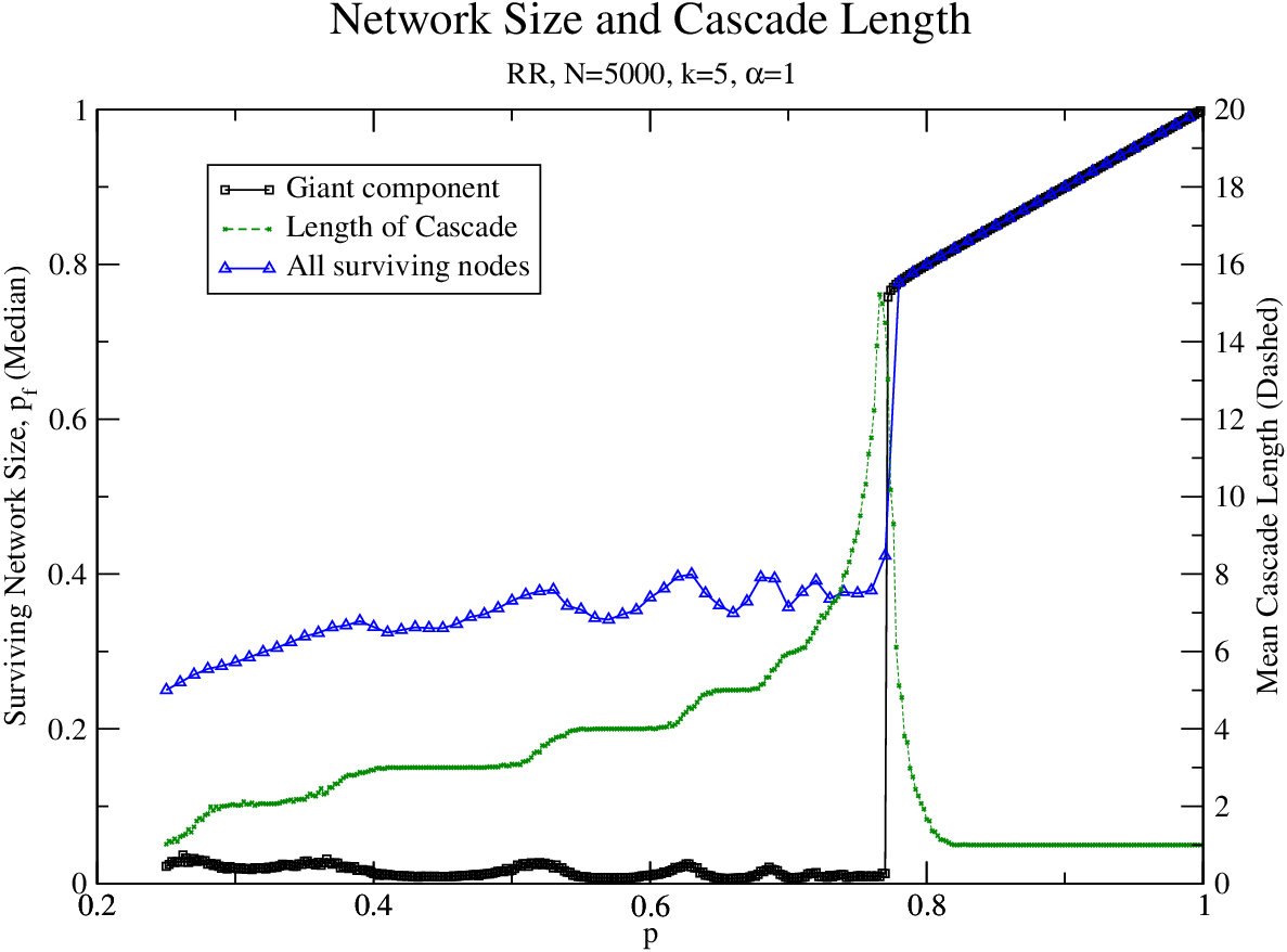
The steps in the cascade length, and the associated fluctuations in the number of survived nodes for are caused by the discreteness of the number of cascades neccessary to approach the percolation transition of the network starting from the initial fraction of survived nodes, . If after the -th step is still larger than the percolation transition, a giant component may still exist, but its size is small enough for the betweennees of its members to be still below the maximal betweeenness. As increases, also increases, the size of the giant component increases and some of its memberes may exceed the maximal betweenness. At this point an additional, step may become necessary, and the average will be in between the large and the small and starts to decrease together with the giant component, while average number of cascades starts to increase from to .
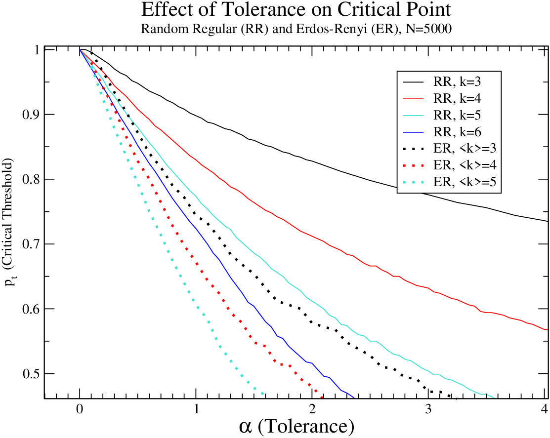
We studied how the value of the size of the threshold initial attack depends on the different values of the tolerance for graphs with different connectivity. In the case of random regular graphs (RR), we show data for different values of the degree . In the case of Erdös-Renyi graphs (ER) we present data for different values of the average degree (Fig. 2). It can be seen, as we would expect, that as the tolerance increases, the network becomes more resilient and decreases. This feature is common to both types of networks. For the same tolerance, the ER graphs with the average degree are in all cases more resilient than the RR graphs with degree . We will show later that at sufficiently high tolerances, the collapse of the network changes its nature, and we observe a more gradual second-order transition.
III General Results
In order to better understand the behavior of a graph under a massive attack, we studied the distribution of the betweenness of the nodes for the graphs before the initial attack and just after it (before the cascade of failures takes place). We start our analysis with the simpler case of RR graphs. Before the initial attack, the betweenness distribution of RR graphs is a sharp Gaussian curve centered around its mean [17]. After the initial attack the distribution presents a structure in which it is divided into a number of wider curves, each of which follows a nearly-normal distribution, although with a much larger standard deviation (Fig. 3). The division of the single Gaussian curve into many curves as a result of the initial attack is an important result of this work. The betweenness of a node surviving the initial attack is essentially determined by the number of its surviving immediate neighbors, denoted as . Specifically, the betweenness is approximately proportional to , which is similar to, although not identical to, the results found by Goh et al. for scale-free networks [10], in which a scaling relationship between the betweenness of a node and its degree was found. A theoretical argument for this dependence is given in section V, and we present a comparison with our numerical simulations in Fig. 4. After the initial attack, our random regular graph loses a fraction of its nodes, causing the number of surviving first neighbors to vary from node to node. Most of the nodes for which all of the first neighbors survive will have their betweeness increased due to the attack. In contrast, those nodes with neighbors that were destroyed in the initial attack will see their betweenness decrease.
Accordingly, our results show that the majority of the nodes with all of their neighbors surviving are the nodes whose betweenness will exceed the maximum betweenness and will fail first due to overload, thus driving the phenomena seen in the failure of the network (see Fig. 3).

Figure 3 provides a lower bound for the value of displayed in Fig. 2 for RR(graphs). Indeed, if we neglect the spread in values of , we can assume that gives a good approximation for , but due to the spread . Since both and are decreasing functions of , for sufficiently large , the same is true for the inverse functions. Thus implies . More accurate estimates would require the knowledge of the standard deviation of , which requires additional investigation, which goes beyond the scope of the present paper.

In Erdös-Renyi (ER) graphs, we find similar catastrophic failures of the network. However, the mechanism of the failure is slightly different. Because the nodes have different initial degrees, they also have very different initial loads and, thus, different maximum loads. As mentioned (and showed later in section V and Appendix A), nodes of lower initial degree will start with lower betweenness and, correspondingly, lower maximum load. The initial attack, however, will cause a greater proportional increase in the betweenness of low-degree nodes than in high-degree nodes, as shown in Fig. 5, provided, in each case, that all neighbors survive. This will affect the behavior of ER graphs and the way in which they disintegrate. The low-degree nodes fail first (in earlier stages of the cascade and with smaller attacks), causing further fragmenting of the network (see Fig. 6).
If the attack is widespread enough ( ), this fragmentation causes the high-degree nodes to also fail. This multistage phenomenon does not appear to be operative to the same extent in RR graphs; in those graphs, relatively few nodes fail before the point where the cascade of failures becomes catastrophic, while in ER graphs, the decline in the number of nodes in the giant component is more gradual as illustrated in Figure 7; the low-initial-degree nodes fail first, followed by the hubs. Again, the curve in Fig. 5, provides the lower bound for for the ER graphs.

IV Features of the Cascades
IV.1 Progress of Cascade
Immediately after a massive attack near , the few nodes with the greatest increase in betweenness fail. As they fail, other nodes increase in betweenness, and also fail. Soon, the network reaches a point of catastrophic failure, in which many nodes fail in each stage of the cascade (Fig. 7). However, there is an important difference between RR and ER graphs. RR graphs have a much more pronounced initial part of the cascade, in which only a few nodes fail. In ER graphs, instead, we observe faster degradation of the network from the start of the cascades. This is due to the difference in initial degrees; as described, nodes with low initial degrees are most affected by the initial attack. They thus fail first, in the early stages of the cascade. Once they fail, the high-degree nodes fail. This feature is clearly displayed in Fig. 6, where the number of nodes surviving each stage of the cascade in an ER graph has been studied as a function of their initial degree.


IV.2 Order of Transition
At high values of , the fragmentation of the network due to the failure of a few nodes can never cause a catastrophic cascade of failures. This is because the betweenness presents a maximum as a function of the fraction of surviving nodes (see Figs. 4 and 5). Note that the average betweenness per node in the giant component is L, where is the number of nodes in the giant component and L is the average path length in the giant component. As fewer nodes survive, the network becomes fragmented, leading to longer path lengths and thus a larger average betweenness. However, at the same time, the fraction of nodes in the giant component decreases, as nodes become isolated due to the widespread destruction. These isolated nodes do not contribute to the betweenness; they do not have paths reaching the nodes in the largest component. Thus, as fewer nodes survive the initial attack, the betweenness decreases. When very few nodes survive, the second effect dominates, and the mean betweenness of nodes decreases with further destruction. In a first-order transition, the original attack causes nodes to fail due to overload, which will cause the mean betweenness to increase. This in turn will cause more destruction; this cascading effect is the scenario that will lead to a first-order transition.
However, as long as is sufficiently high to prevent the network from failing at the point of maximum mean betweenness, the original attack will not cause further failures. Thus, the network will not fail due to a first-order transition. Instead, it will fail due to a second-order transition when the initial attack and associated overload reaches the percolation threshold (which, for random regular graphs, occurs at .) We define the for this second-order transition as the point where the cascade reaches a maximum in length, analogous to the criterion for first-order transitions.
This shift from first-order to second-order scenarios occurs at the value of where we would expect to equal the fraction of surviving nodes that yields the maximum mean betweenness. That is, if is small enough such that the mean betweenness decreases as decreases, we will only see a second-order transition, as the fraction of nodes in the giant component decreases to zero due to percolation. In the vicinity of this point, we can see the shift from a first-order transition to a second-order transition as increases and decreases (See Fig. 8). Thus, the transition between first and second order will occur when is so low that further cascades decrease the average betweenness, and the only failure possible is due to the network reaching the percolation threshold, and not cascading overload.

IV.3 Size Dependence of the Transition Point
The logarithmic dependence of the betweenness on the system size produces a strong logarithmic dependence of the transition point on the size of the system , and also changes the location of the critical point at which the first order phase transition switches to a second order percolation transition. Fig. 9 (a) shows the behavior of for RR graphs (), for . One can see that the larger networks becomes more vulnerable than the smaller ones. This phenomenon is similar to the one observed in [9] for high dimensional interdependent lattices. For all values of , the curves approach the critical point from above. Note that this value is almost independent of . Since for larger , these curves are going higher, they reach the critical point at larger values of . Figure 9 (b) shows the increase of as a function of the size of the system for different . One can see that grows approximately linearly with above the critical point value .


V Analytical Calculations of the betweenness
In order to estimate the betweenness, we need to define an exterior and a shell. We define as the fraction of nodes more than nodes away from a central node and as the fraction of nodes that are exactly nodes away. We further define as the fraction of nodes that are isolated from the giant component of the network. These are all expressed as fractions of , the size of the decimated network. By definition,
| (1) |
In the rest of this section, we will illustrate our findings for the case of random regular graphs, and will collect results from Erdös-Renyi graphs in Appendix A.
Following [14], we use the relationship
| (2) |
where is the generating function of the network, is the generating function of the branching proces, and is the inverse of .
In the case of RR graphs this expression becomes,
| (3) |
It is known [11] that if a random fraction of the nodes are destroyed in a network which initially had a generating function given by , the generating function of the decimated network becomes for the same function . Thus, for a decimated random regular network with initial degree , we obtain
| (4) |
This relationship allows us to create shells of nodes around a central node which ends up with surviving neighbors after the initial attack. Setting by definition, and doing a Taylor expansion of around 1, and using Eqs. (1) and (4) for the case , we obtain for the case of RR graphs
| (5) |
With these equations, we are now in a position to calculate the betweenness of a node with surviving neighbors. In order to proceed, we first study the contribution to the betweenness from paths that leave another node and travel through , where is a distance away from (Fig. 10) To do so, we recreate the graph, using as a new ”central node”, around which we build shells. When we recreate the graph around , our original node is in a shell a distance away, and of the nodes in the network belong to the giant component, but are farther away from than the original node is. The shortest path between and any of these nodes in the -exterior (of ) must pass through (or originate in) the -shell, and then travel from there through a link to the -shell. We will assume that each of these links between the and shells (depicted as arrows in Fig. 10(a)) carries an equal amount of traffic.


of these links branch out of the original node ; while an average of links branch out from the other nodes (different from ) in the -shell. Thus, the contribution to the betweenness of due to a single node a distance away is
| (6) |
In this expression, the numerator of the fraction is the number of links that branch out from the node and the denominator is the total number of links that branch out from all the nodes in the -shell of .
This expression contains a slight error; the actual number of links that branch out of ’s -shell is a random variable with a mean at the value given. For computational simplicity, we treat the mean of the fraction as the fraction of the means. This simplification causes errors at low values of , where there is a greater variation in the denominator (Fig. 4)). Taking a second order Taylor expansion of Eq. (6), we find a correction factor of
| (7) |
While we have not calculated directly, the approximation should be noted.
With our value of for the betweenness of a node due to paths leaving a single node , we now make an identical argument for each node a distance away from , for each value of (Fig. 10). In order to do that, we must perform a sum over all . This requires calculating the probability distribution of for a given node . Node will have surviving neighbors with probability [14]
| (8) |
where is the overall fraction of nodes in the network with surviving neighbors, or . Summing over all and all we find that the total betweenness is
| (9) | |||||
| (10) |
This is the closest approximation we have for the betweenness of a node and the equation we use in Fig. 4. Note that is proportional to and is approximately proportional to , giving us the dependence of the betweenness discussed in section III
For large or , we can simplify the denominator in Eq. (6) and average over all (again, introducing a slight error term due to equating the fraction of the averages with the average of the fractions), leading to an average value of for each :
| (11) |
and thus, combining Eqs. (10) and (11),
| (12) |
Note that for , the two fractions are near unity, and we are left with the intuitive result that the mean betweenness will be the average path length, which we will call , multiplied by the network size. This follows from the observation that can be written telescopically as . For other values of , note that for small , , and thus, for (that is, the betweenness of a node in an RR graph with all of its neighbors surviving),
| (13) |
where , as earlier, is , or the total number of nodes in the giant component. We have explicitly written out this prefactor here, to more clearly identify the dependence of our result on Using results from [17], we finally obtain for the betweenness of a node in a random regular graph of degree
| (14) |
While this analysis has been illustrated with random regular graphs, the results also hold true for any random graph, mutatis mutandis, and in Appendix A we reobtain them for Erdös-Renyi graphs.
These results are confirmed within 5%, for , where this approximation is most accurate. Note that the betweenness of the nodes with all of their original neighbors intact increases as approximately , which is the primary cause of network failure.
VI Localized Attack
According to our theory, the network becomes vulnerable because of the variation in the number of surviving neighbors in the nodes. Thus, a localized attack, in which most nodes’ neighbors are unaffected, will be less effective than a comparable random attack. We implement this local attack by selecting a random node in the network. This node is destroyed, and the destruction spreads along the network’s links to each of its neighbors with probability , a measure of the locality of the attack. When the attack reaches a neighboring node, that node is also destroyed, and the damage spreads to its neighbors with the same probability . Once nodes are destroyed, the initial attack ceases, and we begin to evaluate the failure of nodes due to overload. This allows us to interpolate between the case of a totally random attack and a totally localized attack with . Simulations show (Fig 11), as we expected, that a network can survive a local attack, even when a random attack of the same strength would have caused the network’s collapse.

Other models have assumed that the destruction wrought by an initial attack often spreads to the attacked nodes’ neighbors first ([12, 13]). However, our results show the opposite in this model; the nodes closest to the destruction are the least likely to be overloaded. This is confirmed by the progression of the cascade in the case of a localized attack. After the initial attack, the nodes farthest from the center of the destruction are the first nodes to fail. Only after they fail do the inner nodes, near the nodes destroyed in the initial attack, fail (Fig. 12). This difference emphasizes the difference between the random networks and the networks embedded in space for which the opposite effect is observed.[18].

VII Conclusion
We have studied, both computationally and analytically, the effects of widespread attacks on networks that are susceptible to fail due to betweenness overload. We study the fraction of survived nodes at the end of the cascade as function of the strength of the initial attack, measured by the fraction of nodes , which survive the initial attack for different values of tolerance in random regular and Erdös-Renyi graphs. We find the existence of first order phase transition line on a plane, such that if the cascade of failures lead to a very small fraction of survived nodes and the giant component of the network disappears, while for , is large and the giant component of the network is still present. This feature of the cascading failures is similar to the phenomenology found in other models of cascading failures: i.e. bootstrap percolation[19, 21, 22, 20] k-core percolation[22] and mutual percolation in interdependent networks[23, 24, 25]. Exactly at the function undergoes a first order discontinuity. We find that the line ends at critical point , in which the cascading failures are replaced by a second order percolation transition. We analytically find the average betweenness of nodes with different degrees before and after the initial attack, investigate their roles in the cascading failures, and find a lower bound for . The dynamics of cascading failures indicates the existence of a latent period of cascading failures, during which only a few overloads occur at each stage of the cascade. This latent period is more pronounced in RR graphs than in ER graphs. A similar latent period is present in a more realistic model of overloads in the power grid based on a direct current approximation (DC)[26]. Another similarity between the Motter and Lai model and the DC model of the power grid is a complete clusterization of the network at the end of the cascade. In both models, the giant cluster remains to be the most vulnerable until the last stages of the cascade. In the small clusters of the Motter and Lai model, nodes have low betweenness and, thus, do not suffer from overloads, without adding to global transport in the network. In the power grid model, small self-sustaining islands are likely to survive, because local transmission lines connecting neighboring consumers and producers are less likely to develop overloads than lines connecting distant parts of the network, which may develop a huge imbalance of production and consumption.
Our main finding is that the degree of a node is the primary determinant of its betweenness, and thus its risk of overloading. This shows the fragility of nodes with many surviving neighbors, and of nodes with low initial degrees in non-regular networks. This knowledge can be used to stop cascades in their track, or to easily identify the most vulnerable nodes. This result has led to new insights on the critical point, at which the transition shifts from first-order to second-order, and the effect of the degree of the network, the degree distribution, the size of the network, and the tolerance on the stability of the network.
We also study the difference of cascading failures caused by local attacks and random attacks on randomly connected networks. We find that localized attacks are less destructive than random attacks, which is opposite to the behavior of spatially embedded networks [18].
VIII Acknowledgements
Our research was supported by HDTRA1-14-1-0017. SVB acknowledge the partial support of this research through the Dr. Bernard W. Gamson Computational Science Center at Yeshiva College.
IX Appendix A- Calculation of Betweenness for the Erdös-Renyi model
For the case of Erdös-Renyi graphs, the expression equivalent to (4) becomes
| (15) |
and the Taylor expansion equivalent to (5) is
| (16) |
The shell analysis for the contribution of a single node to the betweenness (equivalent to Eq. (6) yields
| (17) |
while equation (10) for the total betweenness still remains valid.
| (19) |
| (20) |
for Erdös-Renyi graphs, where represents the average degree before the attack.
References
- [1] R. Albert, I. Albert, and G. L. Nakardo. Phys. Rev. E, 69 025103 (2004).
- [2] A. E. Motter and Y.C. Lai. Phys. Rev. E, 66, 065102 (2002).
- [3] A. E. Motter. Phys. Rev. Lett., 93, 098701 (2004).
- [4] J.-W. Wang, L.-L. Rong, Safety Sci., 47 1332-1336 (2009).
- [5] P. Crucitti, V. Latora, and M. Marchiori, Phys. Rev. E, 69, 045104 (2004).
- [6] H. Zhao and Z. Y. Gao. Eur. Phys. J. B 57, 95-101 (2007).
- [7] L. Zhao, K. Park, Y. Lai. Phys. Rev. E 70, 035101 (2004).
- [8] B. Wang, B. J. Kim. Euro. Phys. Lett. 78, 48001 (2007).
- [9] S. Lowinger, G. A. Cwilich, S. V. Buldyrev, , Phys. Rev. E 94, 052306 (2016).
- [10] K.-I. Goh, B. Kahng, and D. Kim. Phys. Rev. Lett. 87 278701 (2001).
- [11] M. E. J. Newman, Phys. Rev. E, 66, 016128 (2002).
- [12] C. D. Brummitta, R. M. D’Souzab, and E. A. Leichtf, Proc. Nat. Acad. Sci. 109 E680-E689 (2011).
- [13] W. X. Wang and G. Chen, Phys. Rev. E 77, 026101 (2008).
- [14] J. Shao, S. V. Buldyrev, L. A. Braunstein, S. Havlin and H. E. Stanley. Phys. Rev. E, 80, 036105 (2009).
- [15] M. E. J. Newman, Networks: An Introduction, (Oxford University Press, USA 2010).
- [16] R. Cohen and S. Havlin, Complex Networks: Structure, Robustness and Function, (Cambridge University Press, Cambridge, 2010).
- [17] M.E.J. Newman, S. H. Strogatz, and D. J. Watts. Phys. Rev. E 64, 026118 (2001).
- [18] J. Zhao, D. Li, H. Sanhedrai, R. Cohen, S. Havlin, Nature Communications 7, 10094 (2016)
- [19] D. J. Watts, Proc. Natl. Acad. Sci. USA 99, 5766 (2002).
- [20] J. P. Gleeson, and D. J. Cahalane, Proc. SPIE 6601, 66010W (2007).
- [21] G. Baxter, S. Dorogovtsev, A. Goltsev, and J. Mendes, Phys. Rev. E 82, 011103 (2010).
- [22] G. Baxter, S. Dorogovtsev, A. Goltsev, and J. Mendes, Phys. Rev. E 83, 051134 (2011).
- [23] S. V. Buldyrev, R. Parshani, G. Paul, H. E. Stanley, and S. Havlin, Nature 464, 1025 (2010).
- [24] M. A. Di Muro, S. V. Buldyrev, H. E. Stanley, and L. A. Braunstein, Phys. Rev. E 94, 042304 (2016).
- [25] M. A. Di Muro, L. D. Valdez, H. H. Aragao Rego, S. V. Buldyrev, H. E. Stanley and L. A. Braunstein, Sci. Rep. 7, 15059 (2017).
- [26] R. Spiewak, S. V. Buldyrev, Y. Forman, S. Soltan, G. Zussman, arXiv:1609.07395 (2016).