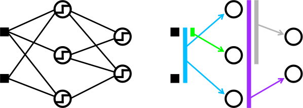
The general idea we adopt is to build connectionist models with the base units being not neurons but kernel machines. This is mathematically viable since in an NN, any neuron can be directly replaced by a kernel machine without altering the architecture and functionality of the network. An illustration of this kernelization procedure is provided in Fig. 1. In this way, one can kernelize an NN to any degree: a node, several nodes, a layer, several layers, or the entire network.

KN is flexible in the sense that one can inject prior knowledge into the architecture design, as is done for NNs. KN inherits the expressive power of the original NN since a kernel machine is a universal function approximator under mild conditions (Park & Sandberg, (1991); Micchelli et al., (2006)). Moreover, KN works in a more mathematically intuitive way since each base unit is a simple linear model in an RKHS.

Further, a general criticism toward kernel methods in machine learning is that their performance usually relies heavily on the parameterization of the kernels used. This issue is mitigated in KN, thanks to the introduction of connectionism. To be specific, KN performs nonparametric kernel learning alongside learning to perform the given task. Indeed, to build the network one only needs generic kernels, but in a connectionist model, the kernels on the non-input layers admit the form $\kernelwa{\vfnwa{F}{\vctr{x}}}{\vfnwa{G}{\vctr{y}}}$, where $\vfn{F}\cm\vfn{G}$ are some other trainable submodels. The fact that $\vfn{F}\cm\vfn{G}$ are trainable makes this kernel “adaptive”, mitigating to some extent any limitation of the fixed generic kernel $k$. The training of $\vfn{F}$ and $\vfn{G}$ makes this adaptive kernel optimal as a constituent part of the corresponding kernel machine for the task the network was trained for. And it is always a valid kernel if the generic kernel $k$ is. Note that observations similar to this one have been made in different contexts by, for example, Huang & LeCun ((2006)) and Bengio et al. ((2013)), we include it here only for completeness.

As a more concrete example, we now define a fully-kernelized $l$-layer MLP, which we will specifically refer to as kernel MLP (kMLP).¹¹ 1 A PyTorch-based (Paszke et al., (2017)) library for implementing KN and the proposed layer-wise training algorithm is available at: https://github.com/michaelshiyu/kerNET.

The $l$-layer kMLP is defined as follows. For $i\geq 1$, the $\ith{i}$ layer in a kMLP, denoted $\vfnsub{F}{i}$, is an array of $d_{i}$ kernel machines: $\vfnsub{F}{i}:\spcsup{R}{d_{i-1}}\to\spcsup{R}{d_{i}},\vfnwasub{F}{\vctr{x}}{i}=\paren{\fnwadub{f}{\vctr{x}}{i}{1}\comma\fnwadub{f}{\vctr{x}}{i}{2}\comma\ldots\comma\fnwadub{f}{\vctr{x}}{i}{d_{i}}}$ with the $\fndub{f}{i}{j}$ all using kernel $k_{i}$. Let $\vfnsub{F}{0}$ be the identity map on $\spcsup{R}{d_{0}}$, each $\fndub{f}{i}{j}:\spcsup{R}{d_{i-1}}\to\spc{R}$ is a hyperplane in RKHS $H_{i}$: $\fnwadub{f}{\vctr{x}}{i}{j}=\innersub{\vctrsub{w}{\fndub{f}{i}{j}}}{\vfnwasub{\phi}{\vfnsub{F}{i-1}\circ\cdots\circ\vfnwasub{F}{\vctr{x}}{0}}{i}}{H_{i}}+b_{\fndub{f}{i}{j}}\comma\vctrsub{w}{\fndub{f}{i}{j}}\in H_{i}\comma b_{\fndub{f}{i}{j}}\in\spc{R}$. The set of mappings

defines an $l$-layer kMLP.

In practice, $\vctrsub{w}{\fndub{f}{i}{j}}$ is usually not accessible but can be approximated using, for instance, $\sum_{n=1}^{N}\alpha_{i\cm n}^{j}\vfnwasub{\phi}{\vfnsub{F}{i-1}\circ\cdots\circ\vfnwasub{F}{\vctrsub{x}{n}}{0}}{i}$, where the $\alpha_{i\cm n}^{j}\in\spc{R}$ are the learnable parameters.²² 2 The optimality of this expansion can be justified in the following layer-wise setting by directly applying the representer theorem (Schölkopf et al., (2001)).

We give a bound on the model complexity of an $l$-layer kMLP using a well-known complexity measure called Gaussian complexity (Bartlett & Mendelson, (2002)). In particular, the bound describes the relationship between the depth/width of the model and the complexity of its hypothesis class, providing insights into the effect of kernelization on the expressive power of the model as well as useful information for model selection. We first review the definition of Gaussian complexity.

Intuitively, Gaussian complexity quantifies how well elements in a given function class can be correlated with a normally-distributed noise sequence of length $N$ (Bartlett & Mendelson, (2002)).

For Proposition 3.2 and the lemma based on which this proposition is proven (Lemma B.2 in Appendix B), we impose the following smoothness assumption on all kernels considered: for each fixed $\vctr{x}\in\spcsup{R}{d_{i-1}}$, we assume that $\kernelwasub{\vctr{x}}{\vctr{y}}{i}$, as a function of $\vctr{y}$, is $L_{i\cm\vctr{x}}$-Lipschitz with respect to the Euclidean metric on $\spcsup{R}{d_{i-1}}$. Let $\sup_{\vctr{x}\in\spcsup{R}{d_{i-1}}}L_{i\cm\vctr{x}}=L_{i}$, which we assume to be finite.

It is worth noting that the model complexity kMLP grows in the depth and width of the network in a similar way as that of an MLP (Sun et al., (2016)). In particular, the expressive power of the model increases linearly in the width of a given layer and roughly exponentially in the depth of the network.

Let the architecture $\spc{F}$ and objective $\tilde{R}$ be given, our greedy learning framework for the two-layer compositional hypothesis class consists of the following steps:

1. 1.

   Finding $\vfndub{F}{1}{\star}$

   1. (a)

      Define an equivalence relation between hypotheses.

   2. (b)

      Give an equivalent definition for $\vfndub{F}{1}{\star}$ under the new equivalence relation.

   3. (c)

      Re-characterize $\vfndub{F}{1}{\star}$ for the given $\spc{F}$ under the given objective $\tilde{R}$.

   4. (d)

      Choose $s\cm u\cm\ell_{1}\cm$ and $\fnsub{\tilde{R}}{1}$ accordingly.

   5. (e)

      Train the input layer to minimize $\fnwasub{\tilde{R}}{\fnwa{s}{\vfnwasub{F}{S_{\vctr}{X}}{1}}\cm\fnwa{u}{S_{Y}}}{1}$.

   6. (f)

      After training, freeze the input layer at, say, $\vfndub{F}{1}{\circ}$.

2. 2.

   Finding $\vfndub{F}{2}{\star}$

   1. (a)

      Train the output layer to minimize $\fnwa{\tilde{R}}{\vfnsub{F}{2}\circ\vfnwadub{F}{S_{\vctr}{X}}{1}{\circ}\cm S_{Y}}$.

We now provide more details for a couple of the listed steps.

In our framework, we use the following definition of equivalence between hypotheses of the input layer:

It is easy to check that this is indeed an equivalence relation. Intuitively, this means that we consider two hypotheses of the input layer to be equally good if the best networks one can build with these two hypotheses minimize the objective function equally well, i.e., when they have the same “potential”. Evidently, this notion of equivalence is proper and sufficient as we have no knowledge of $\vfnsub{F}{2}$ while we train the input layer.

Compared to the original minimizer definition of $\vfndub{F}{1}{\star}$, it is easier to work with the following more concrete definition under the equivalence relation described in Step 1a.

This definition is easier to work with when we later re-characterize $\vfndub{F}{1}{\star}$ because it shrinks the range of $\vfnsub{F}{2}$ we need to consider for each $\vfnsub{F}{1}$ to only the minimizer $\vfnsub{F}{2}$ under that specific $\vfnsub{F}{1}$.

We now provide realizations of the greedy learning framework under a specific family of $\spcsub{F}{2}$ and two classes of objective functions. Note that these realizations are certainly not all that can be derived from our layer-wise framework. We leave the exploration of more such realizations as future work.

Steps 1a and 1b are the same for all realizations. Therefore, the only nontrivial steps in our framework to discuss for specific realizations are steps 1c and 1d.

The specific $\spcsub{F}{2}$ we consider in this section is defined as the set of functions of the following form: $\vfnwasub{F}{\vctr{x}}{2}=(f_{2}^{1}(\vctr{x})\cm\ldots\cm f_{2}^{d_{2}}(\vctr{x}))$, $f_{2}^{j}(\vctr{x})=\innersub{\vctrsub{w}{f_{2}^{j}}}{\phi(\vctr{x})}{H}+b_{f_{2}^{j}}$ with kernel $\kernelwa{\vctr{x}}{\vctr{y}}=\innersub{\fnwa{\phi}{\vctr{x}}}{\fnwa{\phi}{\vctr{y}}}{H}$, $j=1\cm\ldots\cm d_{2}\cm\vctr{x}\cm\vctr{y}\in\spcsup{R}{d_{0}}$, where we have omitted and will continue to omit writing out explicitly the function composition: for example, for $\vctr{x}\in\spcsup{R}{d_{0}}$, we write $\vfnwasub{F}{\vctr{x}}{2}$ in place of $\vfnwasub{F}{\vfnwasub{F}{\vctr{x}}{1}}{2}$. There is no assumption needed on $\spcsub{F}{1}$.

For these realizations, we consider the case $Y\in\setonly{+1\cm-1}$, and we shall use subscript $+$ or $-$ to indicate the class of a particular example, if needed.

Let $d_{2}=1$, write $\fnsub{f}{2}$ in place of $\vfnsub{F}{2}$ accordingly. Let the objective function $\fnwa{\tilde{R}}{\fnsub{f}{2}\circ\vfnsub{F}{1}}$ be $\fnwa{\hat{R}}{\fnsub{f}{2}\circ\vfnsub{F}{1}}+\tau\normsub{\vctrsub{w}{\fnsub{f}{2}}}{H}$, where $\tau>0$ is a hyperparameter that can be chosen as desired and

with $\fnwa{\ell}{\fnsub{f}{2}\circ\vfnsub{F}{1}\comma\paren{\vctrsub{x}{n}\comma y_{n}}}=\max\paren{0,1-y_{n}\fnwasub{f}{\vctrsub{x}{n}}{2}}$, the hinge loss. Let $\kappa=\frac{1}{N}\sum_{n=1}^{N}\ind{y_{n}=+}$. We now re-characterize $\vfndub{F}{1}{\star}$.

Consider function $h:\spcsup{R}{d_{2}}\times\spcsup{R}{d_{2}}\to\spc{R}$ with the property that $\fnwa{h}{\vctr{x}\cm\vctr{y}}$, as a function of $\vctr{x}$ and $\vctr{y}$, has the following properties:

• •

  $\inf_{\vctr{x}\cm\vctr{y}}\fnwa{h}{\vctr{x}\cm\vctr{y}}=b>-\infty$, $\sup_{\vctr{x}\cm\vctr{y}}\fnwa{h}{\vctr{x}\cm\vctr{y}}=d<\infty$, $d>b$;

• •

  $h$ depends only on $\normsub{\vctr{x}-\vctr{y}}{q}$ for some $q\geq 1$, i.e., $\fnwa{h}{\vctr{x}\cm\vctr{y}}=\fnwa{h}{\normsub{\vctr{x}-\vctr{y}}{q}}$;

• •

  $h$ strictly decreases in $\normsub{\vctr{x}-\vctr{y}}{q}$ for all $\vctr{x}\cm\vctr{y}\in\spcsup{R}{d_{2}}\text{ with }\fnwa{h}{\vctr{x}\cm\vctr{y}}>b$.

Define the following SRS loss:

where $p\geq 1$ can be arbitrarily chosen and $\fnwa{g}{y\cm y^{\prime}}=b$ if $y\neq y^{\prime}$ and $d$ if otherwise.

It is easy to see that this loss penalizes the similarity between images of examples under the mapping $\vfnsub{F}{2}\circ\vfnsub{F}{1}$ based on their classes, therefore the name supervised representation similarity.

Let the objective function be

where $\tau>0$ can be freely chosen and $t$ can be any function that strictly decreases in all of its arguments.

For both of the two objectives described above, we may choose, for example, $s$ to be the kernel function $k$, $u$ to be the function defined as $\fnwa{u}{y\cm y^{\prime}}=a$ if $y\neq y^{\prime}$ and $c$ if otherwise, and $\ell_{1}$ to be the SRS loss defined earlier with $g$ set to $u$ and $h$ set to $s$, i.e.,

where $p\geq 1$ can be freely chosen. This of course requires $k$ to satisfy the aforementioned conditions on $h$ for the resulting loss to be a valid SRS loss.

Under this selection of $\ell_{1}$, it is evident that the minimizers of $\ell_{1}$ (and also $R_{1}$) are all equal to $\vfndub{F}{1}{\star}$ by Theorems 4.2 and 4.3. $\tilde{R}_{1}$ can be set to the empirical SRS loss plus an arbitrary regularization term on norms of the weights.

The generalization to a feedforward model with $l$ layers, where $l\geq 2$ can be arbitrary, is trivial. To begin with, treat $\vfnsub{F}{l}$ and $\vfnsub{F}{l-1}\circ\cdots\circ\vfnsub{F}{1}$ as the earlier $\vfnsub{F}{2}$ and $\vfnsub{F}{1}$, respectively. Then work as in the two-layer case to find an objective $\fnsub{\tilde{R}}{l-1}$ for $\vfnsub{F}{l-1}\circ\cdots\circ\vfnsub{F}{1}$. This reduces the $l$-layer problem to an $l-1$-layer problem. Repeat this procedure on the rest of the layers until we return to the original two-layer case.

We can build upon the above realizations an certified (in the sense that the optimality is guaranteed) layer-wise algorithm for training an $l$-layer ($l\geq 2$) feedforward network for classification tasks. In this section, we describe this algorithm and show that it enjoys a geometric interpretation that makes the learning dynamics transparent. Moreover, we show that there is a simple acceleration method for the kernelized non-input layers, making the architecture more practical.

We present this algorithm for binary classification. Nevertheless, as multi-class problems can be reduced to a set of binary classification problems by using either the one-vs-all or the one-vs-one strategy (Schölkopf & Smola, (2001)), an extension of this algorithm to multi-class problems is trivial.

The architecture considered is as follows:

Note that we have made no assumption on the input layer.

For $i<l$, define

where

$p\geq 1$ can be chosen freely, $\tau>0$, $\fnwa{u}{y\cm y^{\prime}}=a$ if $y=y^{\prime}$ and $c$ otherwise, and $t$ can be any function that strictly decreases in all of its arguments.

For $i=l$, define :

where

Then the training algorithm is given in Algorithm 1.

The optimality of this training algorithm is justified by Theorems 4.2 and 4.3 when the $\tau_{i}$ and $k_{i}$ satisfy the corresponding conditions for all $i=1\cm\ldots\cm l$.

We emphasize that this particular training algorithm gives great freedom to the choice of $\vfnsub{F}{1}$: it can be any arbitrary architecture. In particular, it can be a stack of multiple layers in practice. This stack can be trained with an end-to-end method such as BP.

Existing layer-wise pre-training methods such as those proposed in (Hinton et al., (2006)) and (Bengio et al., (2007)) require backpropagation (BP) fine-tuning. This is because, to the best of our knowledge, no optimality guarantee comparable to that provided by BP can be made for these pre-training algorithms. In other words, the layer-wise pre-training commonly used in the deep learning community does not necessarily learn the hypothesis that minimizes the objective function for the network and thus can only be used as an add-on to BP that helps BP converge faster.

In contrast, our work proves such optimality for our layer-wise training scheme in certain specific learning settings and therefore completely removes the need for BP in these settings. To put this in another way, even if one applies BP after performing our layer-wise training, one will not (in theory) end up with a hypothesis that is strictly better than the one learned by the layer-wise learning process in terms of minimizing the objective function of the network.

Coming up with a purely layer-wise substitute for BP is relevant because, as we have mentioned, BP can be computationally expensive and its end-to-end nature makes it practically impossible to precisely trace the source of unsatisfying performance and find out which layer or layers is to be blamed. This can make the architecture search process lengthy and sometimes painful. Furthermore, training all layers simultaneously complicates the parameter space and may introduce more local minima to the learning process, which can be another unwanted factor for gradient descent-based learning. In contrast, a fully layer-wise training process allows one to divide and conquer the learning problem and reveals more useful information about training, mitigating the aforementioned issues to some extent.

We now compare a single-hidden-layer kMLP using simple, generic kernels with the classical SVM and SVMs enhanced by MKL algorithms that used significantly more kernels to demonstrate the competence of kMLP and in particular, its ability to perform well without excessive kernel parameterization. The standard SVM and seven other SVMs enhanced by popular MKL methods were compared (Zhuang et al., (2011)), including the classical convex MKL (Lanckriet et al., (2004)) with kernels learned using the extended level method proposed in (Xu et al., (2009)) ($\text{MKL}^{\text{LEVEL}}$); MKL with $L^{p}$ norm regularization over kernel weights (Kloft et al., (2011)) ($L^{p}$MKL), for which the cutting plane algorithm with second order Taylor approximation of $L^{p}$ was adopted; Generalized MKL in (Varma & Babu, (2009)) (GMKL), for which the target kernel class was the Hadamard product of single Gaussian kernel defined on each dimension; Infinite Kernel Learning in (Gehler & Nowozin, (2008)) (IKL) with $\text{MKL}^{\text{LEVEL}}$ as the embedded optimizer for kernel weights; 2-layer Multilayer Kernel Machine in (Cho & Saul, (2009)) (MKM); 2-Layer MKL (2LMKL) and Infinite 2-Layer MKL in (Zhuang et al., (2011)) ($\text{2LMKL}^{\text{INF}}$).

Eleven binary classification data sets that have been widely used in MKL literature were split evenly for training and test and were all normalized to zero mean and unit variance prior to training. Twenty runs with identical settings but random weight initializations were repeated for each model. For each repetition, a new training-test split was selected randomly.

For kMLP, all results were achieved using a greedily-trained, one-hidden-layer model with the number of kernel machines ranging from 3 to 10 on the first layer for different data sets. The second layer was a single kernel machine. All kernel machines within one layer used the same Gaussian kernel ($\kernelwa{\vctr{x}}{\vctr{y}}=e^{-\normsub{\vctr{x}-\vctr{y}}{2}/\sigma^{2}}$), and the two kernels on the two layers differed only in kernel width $\sigma$. All hyperparameters were chosen via $5$-fold cross-validation. As for the other models compared, for each data set, SVM used a Gaussian kernel. For the MKL algorithms, the base kernels contained Gaussian kernels with 10 different widths on all features and on each single feature and polynomial kernels of degree 1 to 3 on all features and on each single feature. For $\text{2LMKL}^{\text{INF}}$, one Gaussian kernel was added to the base kernels at each iteration. Each base kernel matrix was normalized to unit trace. For $L^{p}$MKL, $p$ was selected from $\{2,3,4\}$. For MKM, the degree parameter was chosen from $\{0,1,2\}$. All hyperparameters were selected via $5$-fold cross-validation.

From Table 1, kMLP compares favorably with other models, which validates our claim that kMLP learns its own kernels nonparametrically hence can work well even without excessive kernel parameterization. Performance difference among models can be small for some data sets, which is expected since these datasets are all rather small in size and not too challenging. Nevertheless, it is worth noting that only two Gaussian kernels were used for kMLP, whereas all other models except for SVM used significantly more kernels.

In this section, we provide empirical results on comparing KN with NN. In the first part, we demonstrate the competence of kernelized NNs and the effectiveness of the layer-wise learning method using kMLPs. We use the proposed layer-wise algorithm derived from our greedy learning framework and Adam (Kingma & Ba, (2014)) as the underlying optimization algorithm. First, we show that this algorithm, albeit only having been certified under certain families of objectives, works well with most popular objective functions in practice. We then compare kMLPs trained with BP and the layer-wise algorithm to show the effectiveness of the latter. Finally, to further showcase the competence of the greedily-trained kernelized models, we compare kMLPs learned layer-wise with other popular deep architectures including MLPs, Deep Belief Networks (DBNs) (Hinton & Salakhutdinov, (2006)) and Stacked Autoencoders (SAEs) (Vincent et al., (2010)), with the last two trained using a combination of unsupervised greedy pre-training and standard BP (Hinton et al., (2006); Bengio et al., (2007)). We also visualize the learning dynamics of greedy kMLPs and show that it is intuitive and simple to interpret. In the second part of the experiments, we partially kernelize the classic LeNet-5 (LeCun et al., (1998)) and compare it with the original to validate our claim that the proposed kernelization and training algorithm is flexible in the sense that it works well with any given feedforward NN architecture and one can freely decide the degree of kernelization. The hidden representations learned from the two models are visualized. We show that the hidden representations learned by the kernelized model are much more discriminative than that from the original.

References

- Bach et al. ((2004)) Bach, F.R., Lanckriet, G.R. & Jordan, M.I. (2004). Multiple kernel learning, conic duality, and the smo algorithm. In Proceedings of the twenty-first international conference on machine learning (p. 6).
- Balduzzi et al. ((2015)) Balduzzi, D., Vanchinathan, H. & Buhmann, J.M. (2015). Kickback cuts backprop’s red-tape: Biologically plausible credit assignment in neural networks. In Aaai ( 485–491).
- Bartlett & Mendelson ((2002)) Bartlett, P.L. & Mendelson, S. (2002). Rademacher and gaussian complexities: Risk bounds and structural results. Journal of Machine Learning Research 3 Nov 463–482.
- Bengio ((2014)) Bengio, Y. (2014). How auto-encoders could provide credit assignment in deep networks via target propagation. arXiv preprint arXiv:1407.7906 .
- Bengio et al. ((2013)) Bengio, Y., Courville, A. & Vincent, P. (2013). Representation learning: A review and new perspectives. IEEE transactions on pattern analysis and machine intelligence 35 8 1798–1828.
- Bengio et al. ((2007)) Bengio, Y., Lamblin, P., Popovici, D. & Larochelle, H. (2007). Greedy layer-wise training of deep networks. In Advances in neural information processing systems ( 153–160).
- Carreira-Perpinan & Wang ((2014)) Carreira-Perpinan, M. & Wang, W. (2014). Distributed optimization of deeply nested systems. In Artificial intelligence and statistics ( 10–19).
- Cho & Saul ((2009)) Cho, Y. & Saul, L.K. (2009). Kernel methods for deep learning. In Advances in neural information processing systems ( 342–350).
- Cortes & Vapnik ((1995)) Cortes, C. & Vapnik, V. (1995). Support-vector networks. Machine learning 20 3 273–297.
- Cristianini et al. ((2002)) Cristianini, N., Shawe-Taylor, J., Elisseeff, A. & Kandola, J.S. (2002). On kernel-target alignment. In Advances in neural information processing systems ( 367–373).
- Fahlman & Lebiere ((1990)) Fahlman, S.E. & Lebiere, C. (1990). The cascade-correlation learning architecture. In Advances in neural information processing systems ( 524–532).
- Gardner et al. ((2015)) Gardner, J.R., Upchurch, P., Kusner, M.J., Li, Y., Weinberger, K.Q., Bala, K. & Hopcroft, J.E. (2015). Deep manifold traversal: Changing labels with convolutional features. arXiv preprint arXiv:1511.06421 .
- Gatys et al. ((2015)) Gatys, L.A., Ecker, A.S. & Bethge, M. (2015). A neural algorithm of artistic style. arXiv preprint arXiv:1508.06576 .
- Gehler & Nowozin ((2008)) Gehler, P. & Nowozin, S. (2008). Infinite kernel learning.
- Glorot et al. ((2011)) Glorot, X., Bordes, A. & Bengio, Y. (2011). Deep sparse rectifier neural networks. In Proceedings of the fourteenth international conference on artificial intelligence and statistics ( 315–323).
- Gönen & Alpaydın ((2011)) Gönen, M. & Alpaydın, E. (2011). Multiple kernel learning algorithms. Journal of machine learning research 12 Jul 2211–2268.
- Hermans & Schrauwen ((2012)) Hermans, M. & Schrauwen, B. (2012). Recurrent kernel machines: Computing with infinite echo state networks. Neural Computation 24 1 104–133.
- Hinton et al. ((2006)) Hinton, G.E., Osindero, S. & Teh, Y.W. (2006). A fast learning algorithm for deep belief nets. Neural computation 18 7 1527–1554.
- Hinton & Salakhutdinov ((2006)) Hinton, G.E. & Salakhutdinov, R.R. (2006). Reducing the dimensionality of data with neural networks. science 313 5786 504–507.
- Huang & LeCun ((2006)) Huang, F.J. & LeCun, Y. (2006). Large-scale learning with svm and convolutional for generic object categorization. In Computer vision and pattern recognition, 2006 ieee computer society conference on ( 1, 284–291).
- Ioffe & Szegedy ((2015)) Ioffe, S. & Szegedy, C. (2015). Batch normalization: Accelerating deep network training by reducing internal covariate shift. arXiv preprint arXiv:1502.03167 .
- Jaderberg et al. ((2016)) Jaderberg, M., Czarnecki, W.M., Osindero, S., Vinyals, O., Graves, A., Silver, D. & Kavukcuoglu, K. (2016). Decoupled neural interfaces using synthetic gradients. arXiv preprint arXiv:1608.05343 .
- Kingma & Ba ((2014)) Kingma, D.P. & Ba, J. (2014). Adam: A method for stochastic optimization. arXiv preprint arXiv:1412.6980 .
- Kloft et al. ((2011)) Kloft, M., Brefeld, U., Sonnenburg, S. & Zien, A. (2011). Lp-norm multiple kernel learning. Journal of Machine Learning Research 12 Mar 953–997.
- Krizhevsky & Hinton ((2009)) Krizhevsky, A. & Hinton, G. (2009). Learning multiple layers of features from tiny images Tech. Rep.. : Citeseer.
- Lanckriet et al. ((2004)) Lanckriet, G.R., Cristianini, N., Bartlett, P., Ghaoui, L.E. & Jordan, M.I. (2004). Learning the kernel matrix with semidefinite programming. Journal of Machine learning research 5 Jan 27–72.
- Larochelle et al. ((2007)) Larochelle, H., Erhan, D., Courville, A., Bergstra, J. & Bengio, Y. (2007). An empirical evaluation of deep architectures on problems with many factors of variation. In Proceedings of the 24th international conference on machine learning ( 473–480).
- LeCun et al. ((1998)) LeCun, Y., Bottou, L., Bengio, Y. & Haffner, P. (1998). Gradient-based learning applied to document recognition. Proceedings of the IEEE 86 11 2278–2324.
- LeCun et al. ((2010)) LeCun, Y., Cortes, C. & Burges, C. (2010). Mnist handwritten digit database. AT&T Labs [Online]. Available: http://yann. lecun. com/exdb/mnist 2 .
- Lee et al. ((2015)) Lee, D-H., Zhang, S., Fischer, A. & Bengio, Y. (2015). Difference target propagation. In Joint european conference on machine learning and knowledge discovery in databases ( 498–515).
- Mairal et al. ((2014)) Mairal, J., Koniusz, P., Harchaoui, Z. & Schmid, C. (2014). Convolutional kernel networks. In Advances in neural information processing systems ( 2627–2635).
- McCulloch & Pitts ((1943)) McCulloch, W.S. & Pitts, W. (1943). A logical calculus of the ideas immanent in nervous activity. The bulletin of mathematical biophysics 5 4 115–133.
- Micchelli et al. ((2006)) Micchelli, C.A., Xu, Y. & Zhang, H. (2006). Universal kernels. Journal of Machine Learning Research 7 Dec 2651–2667.
- Park & Sandberg ((1991)) Park, J. & Sandberg, I.W. (1991). Universal approximation using radial-basis-function networks. Neural computation 3 2 246–257.
- Paszke et al. ((2017)) Paszke, A., Gross, S., Chintala, S. & Chanan, G. (2017). Pytorch: Tensors and dynamic neural networks in python with strong gpu acceleration.
- Pisier ((1999)) Pisier, G. (1999). The volume of convex bodies and banach space geometry ( 94). : Cambridge University Press.
- Raghu et al. ((2017)) Raghu, M., Gilmer, J., Yosinski, J. & Sohl-Dickstein, J. (2017). Svcca: Singular vector canonical correlation analysis for deep learning dynamics and interpretability. In Advances in neural information processing systems ( 6076–6085).
- Rahimi & Recht ((2008)) Rahimi, A. & Recht, B. (2008). Random features for large-scale kernel machines. In Advances in neural information processing systems ( 1177–1184).
- Rumelhart et al. ((1986)) Rumelhart, D.E., Hinton, G.E. & Williams, R.J. (1986). Learning representations by back-propagating errors. Nature 323 6088 533–538.
- Schölkopf et al. ((2001)) Schölkopf, B., Herbrich, R. & Smola, A.J. (2001). A generalized representer theorem. In Computational learning theory ( 416–426).
- Schölkopf & Smola ((2001)) Schölkopf, B. & Smola, A.J. (2001). Learning with kernels: support vector machines, regularization, optimization, and beyond. : MIT press.
- Srivastava et al. ((2014)) Srivastava, N., Hinton, G., Krizhevsky, A., Sutskever, I. & Salakhutdinov, R. (2014). Dropout: a simple way to prevent neural networks from overfitting. The Journal of Machine Learning Research 15 1 1929–1958.
- Sun et al. ((2016)) Sun, S., Chen, W., Wang, L., Liu, X. & Liu, T-Y. (2016). On the depth of deep neural networks: A theoretical view. In Aaai ( 2066–2072).
- Suykens ((2017)) Suykens, J.A. (2017). Deep restricted kernel machines using conjugate feature duality. Neural computation 29 8 2123–2163.
- Suykens & Vandewalle ((1999)) Suykens, J.A. & Vandewalle, J. (1999). Training multilayer perceptron classifiers based on a modified support vector method. IEEE Transactions on Neural Networks 10 4 907–911.
- Tang ((2013)) Tang, Y. (2013). Deep learning using linear support vector machines. arXiv preprint arXiv:1306.0239 .
- Tieleman & Hinton ((2012)) Tieleman, T. & Hinton, G. (2012). Lecture 6.5-rmsprop, coursera: Neural networks for machine learning. University of Toronto, Technical Report .
- Vapnik ((2000)) Vapnik, V. (2000). The nature of statistical learning theory.
- Varma & Babu ((2009)) Varma, M. & Babu, B.R. (2009). More generality in efficient multiple kernel learning. In Proceedings of the 26th annual international conference on machine learning ( 1065–1072).
- Vincent et al. ((2010)) Vincent, P., Larochelle, H., Lajoie, I., Bengio, Y. & Manzagol, P.A. (2010). Stacked denoising autoencoders: Learning useful representations in a deep network with a local denoising criterion. Journal of Machine Learning Research 11 Dec 3371–3408.
- Wilson et al. ((2016)) Wilson, A.G., Hu, Z., Salakhutdinov, R. & Xing, E.P. (2016). Deep kernel learning. In Artificial intelligence and statistics ( 370–378).
- Xiao et al. ((2017)) Xiao, H., Rasul, K. & Vollgraf, R. (2017). Fashion-mnist: a novel image dataset for benchmarking machine learning algorithms.
- Xu et al. ((2009)) Xu, Z., Jin, R., King, I. & Lyu, M. (2009). An extended level method for efficient multiple kernel learning. In Advances in neural information processing systems ( 1825–1832).
- Zhang et al. ((2017)) Zhang, S., Li, J., Xie, P., Zhang, Y., Shao, M., Zhou, H. & Yan, M. (2017). Stacked kernel network. arXiv preprint arXiv:1711.09219 .
- Zhou & Feng ((2017)) Zhou, Z-H. & Feng, J. (2017). Deep forest: Towards an alternative to deep neural networks. arXiv preprint arXiv:1702.08835 .
- Zhuang et al. ((2011)) Zhuang, J., Tsang, I.W. & Hoi, S.C. (2011). Two-layer multiple kernel learning. In Proceedings of the fourteenth international conference on artificial intelligence and statistics ( 909–917).
Appendix A Experimental Setup
The data set rectangles has 1000 training images, 200 validation images 33 3 The last 200 of the training set. Same for other datasets as well., and 50000 test images. The model is required to tell if a rectangle contained in an image has a larger width or length. The location of the rectangle is random. The border of the rectangle has pixel value 255 and pixels in the rest of an image all have value 0. rectangles-image is the same as rectangles except that the inside and outside of the rectangle are replaced by an image patch, respectively. rectangles-image has 10000 training images, 2000 validation images, and 50000 test images. convex consists of images in which there are white regions (pixel value 255) on black (pixel value 0) background. The model needs to tell if the region is convex. This data set has 6000 training images, 2000 validation images, and 50000 test images. mnist (50k test) contains 10000 training images, 2000 validation images, and 50000 test images taken from the standard MNIST. mnist (50k test) rotated is the same as the fourth except that the digits have been randomly rotated. For detailed descriptions of the data sets, see (Larochelle et al., (2007)).
The experimental setup for the greedily-trained kMLPs is as follows, kMLP-1 corresponds to a one-hidden-layer kMLP with the first layer consisting of 15 to 150 kernel machines using the same Gaussian kernel and the second layer being a single or ten (depending on the number of classes) kernel machines using another Gaussian kernel. Hyperparameters were selected using the validation set. The validation set was then used in final training only for early-stopping based on validation error. For the standard MNIST and Fashion-MNIST, the last training examples were held out as validation set. is the same kMLP for which we accelerated by randomly choosing a subset of the training set as centers for the second layer after the first had been trained. The kMLP-2 and are the two-hidden-layer kMLPs, the second hidden layers of which contained 15 to 150 kernel machines. Settings of all the kMLPs trained with BP can be found in (Zhang et al., (2017)). Note that because it is extremely time/memory-consuming to train kMLP-2 with BP without any acceleration method, to make training possible, we could only randomly use 10000 examples from the entire training set of 55000 examples as centers for the kMLP-2 (BP) from Table 2.
In Table 3, we compared kMLP with a one/two-hidden-layer MLP (MLP-1/MLP-2), a one/three-hidden-layer DBN (DBN-1/DBN-3) and a three-hidden-layer SAE (SAE-3). For these models, hyperparameters were also selected using the validation set. For the MLPs, the sizes of the hidden layers were chosen from the interval [25, 700]. All hyperparameters involved in Adam, RMSProp and BN were set to the suggested default values in the corresponding papers. If used, dropout or BN was added to the hidden layers and the best probability for dropout was found using the validation set. For DBN-3 and SAE-3, the sizes of the three hidden layers varied in intervals [500, 3000], [500, 4000] and [1000, 6000], respectively. DBN-1 used a much larger hidden layer than DBN-3 to obtain comparable performance. A simple calculation shows that the total numbers of parameters in the kMLPs were fewer than those in the corresponding DBNs and SAEs by orders of magnitude in all experiments. Like in the training for the kMLPs, the validation set were also reserved for early-stopping in final training. The DBNs and SAEs had been pre-trained unsupervisedly before the supervised training phase, following the algorithms described in (Hinton et al., (2006); Bengio et al., (2007)). More detailed settings for these models were reported in (Larochelle et al., (2007)).
Appendix B Proofs
Lemma B.1.
Suppose are elements from sets of real-valued functions defined on for some , is a subset of their direct sum. For , define as , where , and is bounded and -Lipschitz for each with respect to the Euclidean metric on . Let .
Define
where the are i.i.d. random vectors defined on . We have