Structural Estimation of Behavioral Heterogeneity
Abstract
We develop a behavioral asset pricing model in which agents trade in a market with information friction. Profit-maximizing agents switch between trading strategies in response to dynamic market conditions. Due to noisy private information about the fundamental value, the agents form different evaluations about heterogeneous strategies. We exploit a thin set—a small sub-population—to pointly identify this nonlinear model, and estimate the structural parameters using extended method of moments. Based on the estimated parameters, the model produces return time series that emulate the moments of the real data. These results are robust across different sample periods and estimation methods.
Key words: asset pricing, behavioral finance, extended method of moments, identification, structural model
JEL code: C13, C58, G12, G17
Zhentao Shi (corresponding author): zhentao.shi@cuhk.edu.hk, Department of Economics, 912 Esther Lee Building, the Chinese University of Hong Kong, Shatin, New Territories, Hong Kong SAR, China. Tel: (852) 3943-1432. Fax (852) 2603-5805. Huanhuan Zheng: sppzhen@nus.edu.sg, Lee Kuan Yew School of Public Policy, National University of Singapore, 469C Bukit Timah Road, Singapore 259772. We benefit from in-depth discussion with Taisuke Otsu. We thank Zhenyu Gao, Oliver Linton, Peter Phillips, Michael Zheng Song and Jun Yu for helpful comments. All remaining errors are ours.
1 Introduction
Financial markets undergo cycles of booms and busts. Price fluctuations generate profit opportunities for different investment strategies. No single investment strategy can always triumph—they also experience cycles of gain and loss in response to shifting market environment. It is essential for profit-seeking investors to choose their strategies according to the dynamic market conditions. We try to understand, theoretically and empirically, the impact of information friction on strategy switching. Our model follows the common approach in heterogeneous agent models (HAM), in which an agent selects from multiple investment principles such as the fundamental and technical trading strategies, while we introduce information friction to generate endogenous switching between different strategies.
In this model, every agent receives a private signal—an unbiased forecast about the fundamental value of the risky asset. Given the presence of information dispersion embodied in the realization of the private signal, the agents conceive different evaluations for the same investment strategy. As a result, each agent chooses, from a set of investment strategies, the one that maximizes the expected profit. The agents’ actions reshape the asset price, and the evolutionary environment forces the agents to revise their subsequent choices in the next period. Such dynamic interaction between the agents and the asset price induces behavioral heterogeneity among agents and boom-bust cycles in the financial market.
We formally identify the proposed behavioral model via a thin set—a small subset of the population that reflects some special cases of the model (Khan and Tamer, 2010). We combine the unconditional moments, which involve the whole sample, with those conditional moments motivated from the thin sets. The two kinds of moments differ in the rates of convergence, so that the standard asymptotic theory for generalized method of moments (GMM) is not directly applicable. We employ extended method of moments (XMM) (Gagliardini et al., 2011) for estimation and statistical inference.
Applying XMM to historical observations of the Standard and Poor 500 index (S&P 500), we estimate and test our structural model in several sample periods. The predicted returns from the model closely match the real data in terms of the mean, standard deviation, skewness and kurtosis. Furthermore, we find empirical evidence that supports the evolutionary trading heterogeneity driven by information dispersion. When the price is relatively close to the fundamental value, an investment strategy based on the historical price trend is popular in the market. When the asset is excessively mispriced, however, the agents tend to switch to a fundamental strategy to pursue higher expected profits; their collective actions gradually drive the price toward the fundamental value, which corrects the market.
Our paper makes several contributions to the literature. In terms of modeling, the dynamics in trading heterogeneity has been modeled by latent boom-burst market states (Chiarella et al., 2012), real business cycles (Lof, 2012), and switching stochastic processes (Brock and Hommes, 1998). In particular, Markov transition of discrete regimes is popular in modeling the switching processes, and finds many empirical applications in the stock market, commodity market and derivative market (Frijns et al., 2010; Jongen et al., 2012; Ter Ellen et al., 2013; Eichholtz et al., 2015). While these empirical papers directly model the aggregate time series, they leave unexplained why some agents switch their strategies but the others do not. Our new model combines He and Zheng (2016)’s microeconomic mechanism that endogenizes the Markov switching process and Hirshleifer and Thakor (1992)’s prioritization of profit instead of utility for the agency problem in asset management. Built on a microeconomic foundation of individual behavior, our theoretical model provides implication of the aggregate time series.
Econometric identification is the bridge that links the economic structural model and the data. Well-known is the difficulty to check identification in nonlinear models (Rothenberg, 1971; Newey and McFadden, 1994; Komunjer, 2012). Formal identification is largely missing in the literature of HAM, where nonlinearity is the rule rather than the exception. While following the convention of HAM, we construct our model with identification in mind. The switching between the fundamental and technical strategies opens the opportunity for us to scrutinize in “slow motion” the instant, or the thin set, when the market is overwhelmed by one strategy. When a single strategy dominates, identification can be easily verified. We explore the thin-set identification and manage to recover all structural parameters in our model. To the best of our knowledge, this is the first paper that formally analyzes and establishes identification in the literature of structural modeling of heterogeneous behavior in the financial market.
In terms of estimation methods, existing empirical works of HAM mostly use nonlinear least squares (Boswijk et al., 2007; Chiarella et al., 2012; Frijns et al., 2010), except that Franke and Westerhoff (2012) utilize the simulated method of moments (SMM). We derive an explicit formula of the pricing mechanism that implies moment restrictions in closed-form, which simplifies and speeds up the estimation. XMM is exactly the right bottle opener for a champagne brewed by the thin-set identification, thanks to the econometricians who crafted it.
The rest of the paper is organized as follows. Section 2 develops the information-driven structural asset pricing model of behavioral heterogeneity. Section 3 discusses identification, data handling, and estimation. Section 4 reports the empirical findings, and compares them with those based on alternative approaches. Section 5 concludes the paper. Moreover, we have prepared an Online Supplement with additional empirical results, extension, implementation, and examples.
2 Information-Based Structural Model
In this section, we summarize the key building blocks of the information-based structural model. Step-by-step derivation of the model is given in Appendix Section A. A continuum (of measure one) of agents trade on one risky asset and one risk-free asset. The logarithm of the fundamental value of the risky asset at period , denoted as , is an exogenous random variable that market participants cannot interfere. It follows a random walk for some , where is independently and identically distributed across with mean and variance standardized as 0 and 1, respectively. Let be the history of the fundamental value. At the beginning of period , each agent receives a private signal , an unbiased forecast of the fundamental value . The noise , where is a strictly increasing distribution function with the support of the real line, its density symmetric around 0, and the variance standardized as 1.
Let be the logarithm of the past price. Both and are public information for all investors at the beginning of time . Each agent consults two financial advisors who conduct fundamental analysis and chartist analysis independently, to which we refer as -advisor and -advisor, respectively. The advisors make forecast according to their own perception of price movement, which may not be consistent with the true price formation mechanism. The -advisor expects the price to respond to the fundamental value. Once she learns the private information from her client, she updates the expected to be , which is an average of and weighted by the precision (the inverse of variance), where measures the precision of private information relative to public information. Believing in the efficient market hypothesis, she expects the period- return to be where . The -advisor maximizes the constant absolute risk aversion (CARA) utility function and recommends the optimal investment flow into the risky asset, where is the trading intensity of the fundamental strategy with respect to asset mispricing.
In the meantime, the -advisor utilizes technical analysis to forecast price movement. Her strategy is based only on the historical price trend, rather than or . Her expected period- return is , where is the reference price derived from certain technical rules. Under the same utility function, the -advisor recommends the optimal investment flow into the risky asset, where is the trading intensity of the chartist strategy. Unlike that varies with , for each individual is the same.
We focus on the fundamental and technical strategies of bounded rationality out of many alternatives for the following reasons. (i) The two strategies are used commonly in practice (Allen and Taylor, 1990). (ii) Models accounting for such two strategies are powerful in explaining financial market phenomena such as bubbles and crashes (Lux, 1995; Huang et al., 2010) and providing empirical specifications that outperform random walk (Chiarella et al., 2012). (iii) Due to resource constraints, it is reasonable to prioritize investment strategies with good tracking records, supported by theoretical or empirical foundations; it is costly to hire a large number of financial advisors to conduct various analysis. (iv) No evidence suggests that other types of analysis consistently outperform fundamental and technical analysis in terms of profitability or utility.
Neither strategy is rational in that they ignore how agents’ trading behavior affects the price. Forming rational expectation is difficult in the current setup due to the uncertainty about the convergence of the price to the fundamental value. It deviates from the rational expectation model, in which the price must return to its value at the terminal period. The fundamental strategy that utilizes private information does not always dominate the chartist strategy because the price—determined by the aggregate action of market participants—may not necessarily reflect the information.
Next, we discuss how the agents select trading strategies. Unlike the financial advisors who care about utility, the agents seek to maximize their investment profit in excess to the risk-free asset (Hirshleifer and Thakor, 1992).11 1 Allowing the agents to have a different target function from financial advisors highlights the contrast between practitioners, who adopt straightforward criteria to swiftly respond to market, and researchers, who focus on sophisticated measures of utility. Our main results still hold when agents maximize CARA utility as their financial advisors do. Let be the expected profit of the fundamental strategy based on the information available at the beginning of period , and be that of the chartist strategy. In our model, we have
| (1) |
An agent chooses the strategy that yields higher expected profit. Due to the constraints on risk exposure and resources, we assume that every agent adopts one and only one strategy. Investors are not confident to select strategies that they are unfamiliar with, especially those insufficiently corroborated by studies or experience. It is therefore reasonable to presume that agents ignore strategies that are not scrutinized by their financial advisors.
Now we set equal and to solve the threshold signals that make agents indifferent between the fundamental and the chartist strategy. The quadratic form in (1) yields the lower bound and upper bound , where . The individual choice of the strategy hinges on the private signal. We assume that the agent will choose the fundamental strategy when she is indifferent between the two options. When the agent will adopt the fundamental strategy and we call her a fundamentalist. When she will take the chartist strategy, and we call her a chartist. Given the distribution of the private signal, the fraction of chartists is
The fraction of fundamentalists is . If in addition is unimodal, an application of the Leibniz integral rule to shows that it strictly decreases in . Since captures the degree of mispricing, the fraction of chartists is relatively large (small) when the market is moderately (excessively) mispriced.
After selecting their preferred strategies at the beginning of period , all agents place their trading orders simultaneously to a market maker. Following Lux (1995), we assume that the market maker adjusts the price according to
where is the marginal impact of aggregate demand on the asset price, is the set of the other structural parameters,22 2 Since , we do not need to include into given the presence of and . and
| (2) |
is the aggregate demand in the market, where is the upper-truncated mean. According to the model, the stock market return follows
| (3) |
The above equation characterizes the asset price movements. It will be the key equation for the empirical estimation.
We apply the market-maker framework, instead of the market-clearing mechanism, because the former enables the nonlinear model to be analytically tractable over multiple horizons while the latter does not necessarily yield a solution for the equilibrium price. Venkataraman and Waisburd (2007) find that the market-maker mechanism performs as well as, if not outperforms, the market-clearing mechanism in terms of generating the efficient price.
We conclude this section by comparing our model with the Markov regime-switching regression. The Markov switching model is originated from Hamilton (1989), and has been extended over the decades (Kim, 1994; Kim and Nelson, 1999), with the latest development endogenizing the latent state variable (Kim et al., 2008; Chang et al., 2017). Regime-switching models are featured by the transition probability among discrete states. In contrast, the microeconomic mechanism in our model dictates the variation of the fraction of agents who adopt either strategy in the dynamic market environment. On the one hand, our approach preserves the Markov property since depends only on , which the econometrician directly observes when analyzing the data, but no other past observations. On the other hand, our approach differs from the Markov regime-switching regression as we do not directly model the aggregate time series. Instead, the aggregate market demand is generated by summing up the individual demand. Furthermore, an agent’s switching between heterogeneous strategies is endogenous, because the threshold of the strategy choice is implied by the profit maximization problem. In other words, we attempt to provide a microeconomic foundation for the association between the latent states and the aggregate time series.
3 Econometric Methodology
A model is judged not only by its microeconomic foundation, but also by its empirical fitness. We push the model to encounter data in this section. We verify that the structural parameters can be identified from the distribution of the observable random variables, and then propose an estimation procedure.
3.1 Thin-Set Identification
The structural model is a description of the data generating process, while the analysis of identification bridges the gap between the theoretical model and the observed data. The unobservable noises in the structural model stem from , which are independently and identically distributed across time. As a result, is strictly stationary according to the model.
In reality, the econometrician observes two time series and . If the observable random variables are truly generated from the theoretical model, can we uniquely determine the value of the “deep parameters” from the joint distribution of ? Obviously, can be directly identified from . We narrow down the question to recovering the parameters by matching the distribution of , which comes from the theory, with the distribution of the observable , where the superscript “r” stands for “real”. Nevertheless, cannot be identified jointly. In view of (2) and (3), if we multiply by a non-zero constant and divide and by the same constant, the resulting in (3) remains. Hence we have to normalize and discuss the identification of the other three parameters .
It is well-known that global identification is often difficult in nonlinear models (Rothenberg, 1971; Newey and McFadden, 1994; Komunjer, 2012). In the literature of HAM, identification of structural parameters is largely ignored. In this paper, we formally establish point identification for this highly nonlinear structural model. We take the thin-set identification approach (Khan and Tamer, 2010; Lewbel, 2016), conditioning on some events that occur on a set of measure zero if the random variables are continuously distributed.33 3 This thin-set identification strategy is not peculiar to our model. In Supplement Section S5, we provide examples in which thin-set identification can be invoked to establish point identification for other HAM models. The key insight for the point identification is that when the event
occurs, the expected return of the chartist strategy becomes zero, and all investors thereby turn to the fundamental strategy. Conditional on , we have and , and can simplify (3) as
| (4) |
where and are observable, and and are explicit functions of the deep parameters. As long as the conditional distribution is not perfectly collinear, we can identify and , and then recover and . The occurrence of highlights the particular instant when the market is overwhelmed by the fundamental strategy, and the identification of and follows.
Once is identified, we can further condition on another event
where . Under the event , we verify in Appendix Section B that (3) becomes
where is strictly increasing, and non-negative when .
Taking the expectation operator on both sides of the above equation, we have
Since are already recovered, in the above equation is the only known parameter. Because the right-hand side is monotonically increasing in for any as long as , the parameter is identified.
The discussion of identification ensures that we can pin down the deep parameters from the observable time series given sufficiently many observations. We proceed to the estimation strategy.
3.2 Moment Conditions
Recall that is the real return and is the return according to the model. If the real data is truly generated from the structural model, the distribution of must be the same as the that of . In reality, the structural model is at best a simplification of the real world.
Moment matching is one of the most popular econometric methods to estimate structural models. We estimate the structural parameter by matching moments of the marginal distribution of returns. First, as is identified from the standard deviation of , we specify the first moment function
since . Next, as the two parameters and can be identified given , we match the conditional mean and variance. Notice that these two moments are implied by the thin-set identification, and conditioning on literally means selecting only the observations such that . Since is continuously distributed, the event happens with probability zero. To avoid the problem of too few local observations, we use a kernel function to assign weights to each observation, as in Smith (2007) and Gospodinov and Otsu (2012). We assign large weights on observations with small and small weights on those with large . Given an appropriate bandwidth , we would have enough observations to guarantee the estimation consistency at asymptotically as . Let be the weight of the -th observation, where is the bandwidth and is the density function of the standard normal. We construct two Gaussian-kernel-weighted moment functions
where is the demeaned , and is defined similarly. On the other hand, the chartist parameter is identified conditional on . The argument for identification of conditional on motivates another kernel-weighted moment function
| (5) |
where . We use the same bandwidth in and for simplicity.
Under the assumption that the model is correctly specified, the moments
pointly identify . However, since are constructed from a sub-population, they only use a small fraction of the data. As a consequence, the rates of convergence of the kernel-weighted sample moments are slower than the usual rate of , so are the rates of the estimated parameters. It is desirable to improve the rate of convergence of these parameter estimates by local identification information.
Following Gagliardini et al. (2011) and Antoine and Renault (2012), we assume local identification in the sense of Rothenberg (1971). That is, is locally identified if there exists an open neighborhood of containing no other that can generate the same distribution. Local identification does not contradict the thin-set identification. Local identification is based on the unconditional information of the population. The thin-set point identification here, however, relies on the conditioning of two special events that form the sub-population.
Assuming local identification, we further construct four unconditional moments with the whole sample. Specifically, we match the mean, variance, skewness and kurtosis of the returns:
We focus on these moments, thanks to the well-documented stylized facts about financial time series, i.e., excessive volatility, negative skewness, and fat tail in returns (Cont, 2001). Under local identification, these unconditional moment functions improve asymptotic efficiency of the estimator.
The construction of the moments gives a clear interpretation of indirect inference (Gourieroux et al., 1993). While is the deep parameter from the structural model, those eight conditional and unconditional moments consist of a set of reduced-form parameters. The principle of indirect inference matches the reduced-form parameters from the observable data and the counterparts from the structural model. Model misspecification can be accommodated by indirect inference, in which the estimated structural parameter is the one that minimizes some distance between the reduced-form parameter from the real world and that from the economic theoretical model. Even though our stylized fundamentalist-chartist model is certainly a simplistic narrative, the estimation will tune the model to its best approximation to the features of the observed return time series.
3.3 Estimation: XMM
The standard theory of GMM requires that all moments converge at rate . Such a premise is violated if we combine the eight moments , . The unconditional moments and conditional ones converge to their population means at different rates. Let be the vector of the moment functions. Evaluated at a neighborhood of the true value, the (scaled) sample unconditional moments for , while the (scaled) sample conditional moments for and . With such a mixture of sample moments converging at various rates, the standard asymptotic theory of GMM is inapplicable. Fortunately, Gagliardini et al. (2011) and Antoine and Renault (2012) have developed XMM, an extension of GMM, to explicitly incorporate moments with different rates of convergence. This latest methodological advancement makes the following empirical estimation possible.
We implement XMM by the continuous updating estimator (CUE) (Hansen et al., 1996). Let be the simple sample average of . Define the CUE criterion function as
where , and is the sample long-run variance of . CUE automates the choice of the weighting matrix so that we do not have to track the rate of each sample moment, and the scaling factors in the unconditional moments, and , are also canceled out in .
We denote the XMM estimator as44 4 While standard kernel weight only depends on , here also depends on . In Appendix Section B we explain that it does not affect the asymptotic distribution of .
| (6) |
Under regularity assumptions (see Gagliardini et al. (2011, p.1203) or Antoine and Renault (2012, Theorem 4.3)), if , as , we have
| (7) |
where is the asymptotic variance and it can be consistently estimated by
Regarding the model specification test, Antoine and Renault (2012, Theorem 4.4) prove that this -statistic still follows the usual distribution. With eight moments and four unknown parameters, the degrees of freedom of the distribution is 4.
3.4 Implementation
We use Robert Shiller’s S&P 500 dataset to construct the price and the fundamental (Downloadable at http://www.econ.yale.edu/~shiller/data.htm). The raw time series is taken as the monthly average of the daily closing prices, and is calculated as the present value of all monthly dividend flows according to the Gordon growth model (Gordon, 1959).
Our discussion of the econometric procedure leaves open several choices in the implementation. We discuss these issues one by one. The observed return and the fundamental time series both exhibit upward trends. We have to filter the trends so that we can focus on the fluctuation of the stationary time series. Detrending does not change the behavior of the investors as the growth trend is incorporated in their decision of the quantity they purchase and the strategy they take. For simplicity, we fit a linear trend for each time series and then detrend. We find that the difference in the two trends is very small, which supports the implication of the efficient market hypothesis that the growth rate of and converge in the long run. We observe that detrending in our data preserves the pattern of over- and under-pricing periods as the crossing points of the two raw time series are proximate before and after detrending. Moreover, for the chartist strategy we need a reference price . We use a simple 12-month moving average rule .
We have assumed that the density function of to be symmetric and its support is the real line. Many distributions satisfy these conditions, for example the standard normal, the hyperbolic secant distribution, the Logistic distribution, the Laplace distribution, and the -distributions of degrees of freedom at least 3 (with their variance standardized as 1). While is unobservable, data provides no guidance about the choice of . We select as the standard normal for its theoretical and practical attractiveness. Firstly, under normality the truncated mean function is the (minus) density function of , which is a built-in function in all modern statistical programming languages. Secondly, the normal distribution is favorable in justifying the conditional expectation of in the fundamental strategy. Given and , if the fundamentalist takes a prior distribution , she will attain the posterior distribution which delivers exactly the weighted average rule for the fundamentalist’s expectation of .
Throughout this paper, we use the same set of tuning parameters for all estimation procedures and sample periods. The bandwidth in the kernel-weighted sample moments is set as according to Silverman (1986)’s rule of thumb, where is the sample standard deviation of . The long-run variance is estimated using the Bartlett kernel (Newey and West, 1987); the number of lags in the kernel is chosen as where , with the constant and the rate recommended in Andrews (1991). The rates of these tuning parameters satisfy the requirement for the asymptotic normality, and the estimates are stable in a reasonable range.
When applying XMM to the data, we set the compact parameter space as , which is sufficiently wide for . We must deal with the local optimizers in general nonlinear programming. We try many initial values to enhance the probability of capturing the global minimizer. The initial value for is always the sample mean of . This sample mean is a consistent estimator, although in theory it is not as efficient as the XMM estimator since it does not incorporate the information provided by the other moments. For the other three parameters , the initial value is independently drawn from the uniform distribution over their parameter space. Given a randomly generated initial value, we carry out the nonlinear optimization. We repeat such optimization for 100 times, save each local minimum, and take the smallest one as the global minimum.
4 Empirical Results
In this section, we report the empirical results and compare them with alternative specifications. We first estimate the parameters with a recent time span from January, 1991 to December, 2013, to which we refer as Period 1. We then repeat the estimation procedure for two alternative time spans: January, 1961—December, 1990 (Period 2), and January, 1911—December, 1960 (Period 3) for robustness check.
In Section 4.1, all the eight moments are incorporated in the estimation, to which we refer as the full model. Furthermore, we evaluate the effect of the kernel-weighted moments in Section 4.2, and the mixture of the two strategies in Section 4.3.
4.1 Results from XMM
The time series of the linearly-detrended price and fundamental value in Period 1 are shown in the upper panel of Figure 1. It is apparent that the price is more volatile than the fundamental. The price sometimes deviates significantly away from the fundamental value, which corresponds to boom-bust episodes in the financial history. In the long run, the price tracks the fundamental value in general, which supports the market efficiency theory in a long-term perspective.
We take XMM as our benchmark. We report the XMM estimates of and the two-sided 95% asymptotic confidence intervals in Table 1 for each sample period. All estimates are positive and none of the confidence intervals contains 0, which is consistent with the economic interpretation of these parameters.
The parameters and represent the trading intensity of the fundamental strategy and the chartist strategy, respectively. Based on the estimation results of Period 1, the estimate of means that raising the expected return of the fundamental strategy by 1% increases the investment flow by 0.10% on average. On the other hand, the estimate of implies that 1% change in the expected return of the chartist strategy leads to a 0.61% hike in the investment flow. The estimate of is suggests that investors update their expected fundamental value aggressively by overweighing the private information relative to the common prior on the historical fundamental value, as the private information is more precise than the public information. In terms of the model specification test, the -statistic is 2.22 with the -value 0.70. It does not reject the model, indicating that our model can be a reasonable description of the data generating process for this sample period.
| Period 1 | Period 2 | Period 3 | ||||
| est. | 95% CI | est. | 95% CI | est. | 95% CI | |
| 0.014 | (0.008, 0.020) | 0.007 | (0.006, 0.008) | 0.030 | (0.024, 0.037) | |
| 0.102 | (0.073, 0.131) | 0.171 | (0.141, 0.202) | 0.224 | (0.170, 0.277) | |
| 0.612 | (0.390, 0.835) | 0.758 | (0.607, 0.908) | 1.099 | (0.794, 1.405) | |
| 1.713 | (0.688, 2.739) | 2.021 | (1.127, 2.915) | 3.894 | (2.401, 5.387) | |
| J-stat. | 7.202 | |||||
| p-value | (0.695) | (0.126) | (0.113) | |||
Note: Each column represents the sample period for estimation, where Period 1 is January, 1991—December, 2013, Period 2 is January, 1961—December, 1990, and Period 3 is January, 1911—December, 1960. For each sample period, this table displays the point estimates (est.) of the four structural parameters and the 95% asymptotic confidence intervals (95% CI). The -statistic (-stat.) of the over-identification test and the corresponding -value are also reported. Under the null hypothesis of correct moment specification, the -statistics asymptotically follows . Tables 3 and 4 below follow the same format.
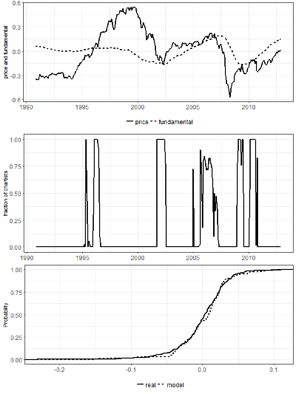
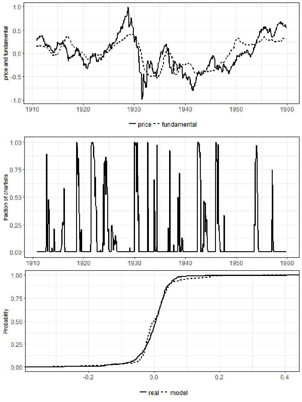
Note: (i) The upper panel shows the linearly detrended price and fundamental value . (ii) The middle panel displays the fraction of chartists according to the full model, computed as . (iii) The lower panel plots the ECDF of the real time series , , and that of the predicted , . Figures 2 and 3 below follow the same format.
Besides the values of the structural parameters, we are also interested in the endogenous switching of the financial agents between the chartist and fundamental strategies. It is illustrated in the middle panel of Figure 1. Consistent with the model’s prediction, the market is dominated by fundamentalists when the asset is excessively mispriced, and by chartists when the price moves more closely around the fundamental value. How agents switched between the heterogeneous strategies during the recent global financial crisis is of particular interest. When the market was booming during 2005–2007, many agents clustered to be chartists, who traded on price trends. When the trend was reversed in late 2007, the market fraction of chartists declined sharply. Fundamentalists prevailed the market in 2008–2009, the most volatile years during the global financial crisis. In that episode, financial assets were overwhelmingly underpriced (as illustrated in the upper panel of Figure 1), and fundamentalists had accumulated strong buying force that drove the price up toward its fundamental value. However, the price may not converge to the fundamental value immediately after the fundamentalists occupy the market. The presence of information friction produces such inertia in our model. No similar patterns of switching was found during the dot-com crisis. In the early period of dot-com bubble formation, chartists dominated the market. As the asset became more and more overpriced, agents switched to fundamentalists. The bubble continued to grow even after fundamentalists fully occupied the market. In a highly noisy environment, some fundamentalists might wrongly extrapolate the asset to be underpriced even if it was actually overpriced.
| Mean | Stan. Dev. | Skewness | Kurtosis | ||
|---|---|---|---|---|---|
| Real return | 0.000 | 0.037 | -1.380 | 9.280 | |
| XMM full model | 0.002 | 0.036 | -0.918 | 6.550 | |
| Period 1 | GMM | 0.001 | 0.036 | -1.180 | 9.020 |
| XMM fundamentalist-only | 0.000 | 0.029 | -0.291 | 2.460 | |
| XMM chartist-only | 0.000 | 0.089 | -1.450 | 5.990 | |
| Real return | 0.000 | 0.036 | -0.786 | 4.970 | |
| XMM full model | 0.000 | 0.041 | -0.214 | 4.340 | |
| Period 2 | GMM | -0.001 | 0.037 | -0.435 | 5.090 |
| XMM fundamentalist-only | 0.000 | 0.028 | 0.261 | 2.330 | |
| XMM chartist-only | 0.000 | 0.107 | -0.670 | 3.310 | |
| Real return | 0.000 | 0.051 | -0.175 | 15.300 | |
| XMM full model | 0.002 | 0.060 | -0.494 | 11.500 | |
| Period 3 | GMM | 0.001 | 0.050 | -0.177 | 13.200 |
| XMM fundamentalist-only | 0.000 | 0.038 | 0.347 | 2.810 | |
| XMM chartist-only | 0.000 | 0.141 | -1.130 | 6.680 |
Note: This table displays the mean, standard deviation (Stan. Dev.), and the standardized skewness and kurtosis of the real returns and the predicted returns. For a sample , the standardized skewness and kurtosis here are respectively computed as and , where and are the sample mean and standard deviation. In each period, the moments of the real returns are computed from the observed time series , , while the other rows are calculated from , , where is the corresponding estimate.
To examine the performance of moment matching, we plug in the estimated parameters into the model to predict the return. In the lower panel of Figure 1, the solid line is the empirical cumulative distribution function (ECDF) of the real data , and the dashed line is the ECDF of the fitted return series . The two ECDF curves closely track each other. As shown in the upper panel of Table 2, the predicted returns generated from XMM have a mean return close to zero, a variance around 0.04, a negative skewness, and a kurtosis that is larger than 3. These sample moments are similar to those of the real return series.
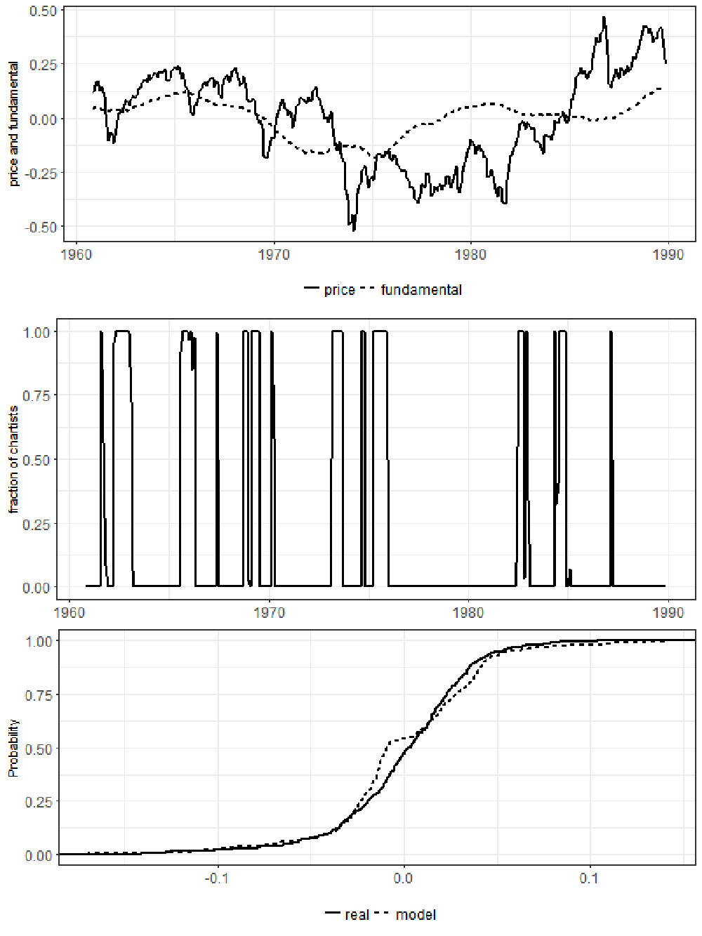
Next, we repeat the same exercises for other sample periods to check the robustness of the empirical results. Figure 2 and the second column in Table 1 display the results of Period 2. Again, the -statistic does not reject the model specification. The estimated coefficients are comparable with those in Period 1. The fitted returns match well with the real data in terms of ECDF and the four moments, as shown in the middle panel of Table 2. Moreover, consistent with the previous results, we observe from the middle panel of Figure 2 that chartists prevailed when the asset was moderately priced, for example in 1976, while fundamentalists dominated the market when the price deviated significantly away from the fundamental, for example in 1978–1982.
Figure 3 and the third column of Table 1 report the results for Period 3, a half century that witnessed the Great Depression. The high volatility in this era is manifest as shown in Table 2, with a kurtosis of 15.30 in the real return, the largest among the three sample periods. In terms of the point estimates, the scale of the estimated coefficients and are larger than those reported in the other two periods, showing that both fundamentalists and chartists responded more sensitively to the expected returns. The estimated coefficient in Period 3 is about twice as large as that in Period 1 or 2, suggesting fundamentalists updated information more aggressively in response to the volatile market. In Figure 3 we again observe the switching from chartists to fundamentalists when the asset was excessively mispriced and from fundamentalists to chartists when the asset was moderately mispriced.
In the following sections, we estimate some simple alternative models and compare the empirical results with those discussed in this section.
4.2 Estimation with Unconditional Moments Only: GMM
The standard GMM utilizes only the unconditional moments in estimation. For comparison, we implement GMM (CUE) with the moment functions , and the results are reported in Table 3. Ignoring , which contains information from the theoretical model, weakens the asymptotic efficiency of parameter estimation. In our context, such efficiency loss is reflected in the confidence intervals—in most cases the confidence intervals of the GMM estimator are wider than their XMM counterparts. In particular, the confidence interval of includes 0, which is highly undesirable since the identification of the parameters relies on a positive . In contrast, when conditional moments are accounted for, the confidence intervals of are clearly deviated away from 0 (see Table 1). In the meantime, with fewer restrictions GMM improves the in-sample fitting. The model emulates the data more closely in terms of moment matching, as shown in Table 2 with the kurtosis of the predicted return closer to that of the real data.
| Period 1 | Period 2 | Period 3 | ||||
|---|---|---|---|---|---|---|
| est. | 95% CI | est. | 95% CI | est. | 95% CI | |
| 0.014 | (0.010, 0.019) | 0.002 | (-0.333, 0.337) | 0.029 | (0.023, 0.036) | |
| 0.109 | (-0.020, 0.238) | 0.055 | (-0.220, 0.330) | 0.280 | (-0.061, 0.621) | |
| 0.676 | (0.359, 0.992) | 0.702 | (0.502, 0.902) | 0.685 | (-0.028, 1.398) | |
| 2.513 | (0.613, 4.413) | 3.363 | (1.405, 5.321) | 2.765 | (0.823, 4.707) | |
| J-stat. | 0.035 | 0.082 | 0.066 | |||
| p-value | (0.852) | (0.774) | (0.797) | |||
Note: Similar to Table 1, this table displays the point estimates (est.) and the 95% asymptotic confidence intervals (95% CI) for each sample period. Since only the unconditional moments are used in the estimation, the -statistics of the over-identification test follows asymptotic distribution under the null.
4.3 Estimation with a Solo Strategy
A common feature of the strategy switching in Figure 1–3 is that fundamentalists dominate the market more frequently than chartists. This observation raises the question of the necessity of introducing the two investment strategies to characterize the price movement. This section explores whether a solo-strategy model is sufficient to capture the price dynamics.
The fundamentalist-only model is a sub-model of the two-strategy benchmark model. When and , the chartist strategy generates zero profit so that no investor will adopt it. The predicted return of the fundamentalist-only model follows (4). Since the kernel-weighted moment functions , remain valid in the sub-model, we estimate the parameters by XMM with the same eight moments as in (6) but setting . With the restriction , the -statistic follows asymptotically under the null.
We report the empirical results in the upper panel of Table 4. The estimates stay positive and statistically significant as the 95% confidence intervals are all above 0. This is consistent with the results from the full model and provides evidence of the presence of the fundamentalist trading in the market. Under the null hypothesis that the fundamentalist-only model is correctly specified, the -statistics are 15.74, 16.44 and 32.15 in Period 1–3, respectively, which are associated with -value less than 1%. The strong rejection means that the fundamental strategy solely is incapable of mimicking the observed price movements. Moreover, in Table 2 the moments of fitted returns are far away from the real ones. In particular, the fitted kurtosis is less than 3 throughout the three sample periods, which contradicts the fat-tail phenomenon observed in the real data.
| Period 1 | Period 2 | Period 3 | ||||
| est. | 95% CI | est. | 95% CI | est. | 95% CI | |
| Fundamentalist-only | ||||||
| 0.015 | (0.010, 0.020) | 0.007 | (0.006, 0.008) | 0.030 | (0.024, 0.036) | |
| 0.084 | (0.060, 0.108) | 0.157 | (0.125, 0.189) | 0.182 | (0.130, 0.233) | |
| 0.612 | (0.378, 0.846) | 1.178 | (0.826, 1.530) | 1.239 | (0.797, 1.682) | |
| J-stat. | ||||||
| p-value | (0.008) | (0.006) | (0.000) | |||
| Chartist-only | ||||||
| 0.009 | (0.002, 0.016) | 0.007 | (0.006, 0.008) | 0.023 | (0.016, 0.031) | |
| 0.871 | (0.792, 0.949) | 1.179 | (1.071, 1.286) | 1.052 | (0.944, 1.161) | |
| J-stat. | ||||||
| p-value | (0.000) | (0.000) | (0.000) | |||
Note: Under the null hypothesis, the -statistic of the fundamentalist-only model follows asymptotic distribution, and that of the chartist-only model is asymptotically. The corresponding -values are so small that the over-identification tests are rejected in all cases at 1% size.
If the fundamentalist-only model is insufficient to capture the real return, how about the chartist-only model? The lower panel of Table 4 displays the XMM estimation results across the three sample periods.55 5 A formal test of the chartist-only model is more complicated than the fundamentalist-only model because the full model precludes due to its presence in the denominator in . The implementation is detailed in Supplement Section S2. The -statistics clearly reject the chartist-only model at any commonly used test size, and the moment matching in Table 2 is poorer than the full model.
In view of the empirical results, neither the fundamentalist strategy nor the chartist strategy alone reasonably matches the data. The mixture of the two trading strategies is effective in improving the model fitting.
5 Conclusion
In this paper, we develop a structural asset pricing model with information-driven behavioral heterogeneity. For this highly nonlinear model, we formally identify the structural parameters via thin-set identification. The thin-set identification and the follow-up estimation techniques are applicable to other heterogeneous agent models involving a mixture of investment strategies.
We estimate the parameters by XMM, and conduct inference for the model specification. The empirical results show that the structural model emulates the S&P 500 index. Investors switch between the fundamental and chartist strategies evolutionarily in response to the dynamic market conditions. Agents tend to cluster toward the chartist strategy when the market environment waxes and wanes, and their collective trading actions cause substantial asset mispricing that sometimes turn into bubbles and crashes. However, when the asset is significantly overpriced or underpriced, agents tend to revert to the fundamental strategy, which corrects the mispricing and restores the market efficiency. The switching is found to be crucial for the empirical fitness of the structural model. Models with only one strategy significantly underperform the structural model in terms of matching the real price movement.
In this Appendix of this paper, we present the step-by-step development of the structural model as well as the derivation of some technical claims in the main text. Moreover, we provide an Online Supplement for additional empirical results, extension, and implementation.
Appendix
Appendix A Complete Description of the Structural Model
This section describes the information-based structural model, summarized in Section 2, step by step.
A.1 Investment Strategies
In each period, the -advisor updates the expected mean of after learning the private information from the agent . She follows a weighted average rule
where the weight is the information precision (the inverse of variance), is the precision of private information relative to public information, and is the expectation of the -advisor conditional on the past public information as well as the private signal . She believes in the efficient market hypothesis under which the price tracks the fundamental value. Let her perceived return be , where is the perceived price to be realized in time . She expects the period- return to be
where the second equality is implies by the efficient market hypothesis, and the last equality by the definitions of and .
The -advisor, on the other hand, employs technical analysis to forecast the price movements. She ignores the private information and the fundamental , even though they are accessible. Let be the -advisor’s expectation conditional on past prices. The -advisor believes that the past price trend captured by would persist in the following period. Let be the chartist’s perceived price to be realized at time , and be the perceived return. Her expected period- return is
Let -advisor’s expected utility , where and is the mean and variance of the wealth , respectively, and is a constant.66 6 Such a functional form can be formally derived under the constant absolute risk aversion (CARA) exponential utility function where is the absolute risk aversion coefficient, and is normally distributed. Such a CARA utility function takes into account the trade-off between risk and return and it facilitates mean-variance analysis. It is widely used in the literature, for example Barberis et al. (ming). Maximizing this utility is essentially maximizing , the difference between the mean and the variance multiplied by a constant.
Given the dynamics of wealth growth , we apply the expected utility function to the -advisor at the beginning of time :
The -advisor who maximizes the expected utility recommends the optimal investment flow
| (8) |
where . We assume that is a constant independent of and . Similar expected utility analysis applies to the -advisor, whose expected utility . As a result, the -advisor recommends the optimal investment flow
| (9) |
where as is assumed to be a constant.
Both the conditional variances of the return are assumed time-invariant for the following reasons.77 7 In Supplement Section S4, we discuss the possibility of extending the theoretical model to allow individual- and/or time-varying conditional variances and its implications to identification and estimation. (i) The traders follow naive investment rules so that their perceived and are not directly observable and the conditional variance cannot be estimated from the data. In such a setup, the constant conditional variance is a convenient assumption following the literature, for example Brock and Hommes (1998, p.1239) and Barberis et al. (ming, p.32), among many others cited in this paper. (ii) The constant conditional variance allows us to derive a simple explicit form for the price dynamics, which simplifies the estimation.
A.2 Choice of Strategies and Aggregation of Demand
Financial advisors advocate optimal investment flows and based on their independent analysis. Each agent is well informed of both strategies as well as the rationale behind (8) and (9). The agent takes only one of the two strategies. The expected profit from a strategy is the product of the expected return and investment flow, i.e.,
for the fundamental strategy, and
for the chartist strategy. The agent prioritizes investment profitability and chooses the strategy that yields a higher expected profit. Let be the threshold such that when . We solve to obtain
and the lower bound and upper bound follow.
Since is a convex function of while is independent of , we have if . The agent, who seeks to maximize her expected profit, acts on the chartist strategy if , whereas she carries out the fundamental strategy otherwise. When , the agent would be indifferent between the two strategies, in which case we assume she adopts the fundamental strategy. As a result, the individual investment flow is
| (10) |
where is the indicator function.
In the market, the fraction of chartists is given by , and the fraction of fundamentalists is . Conditional on the past information and , the aggregate demand of all agents is
where the second equality follows by the definition of in (10), and the last line follows by , the symmetry of .
Appendix B Verification of Technical Results
In Section 2 we have claimed that if is unimodal, then is strictly decreasing in . Here we verify this claim. When , by the Leibniz integral rule
where is the probability density of , and we assume is differentiable. Since is symmetric and unimodal, we have for and for . Given a fixed , if we have
and obviously, for . Parallel analysis applies when .
In Section 3.1 we have claimed that under the event we have . Here we verify this claim. The event implies , under which we have since for any ,
by the symmetry of the density of around 0. The symmetry also implies . Thus in (3) is reduced to
given and .
In Footnote 4 we have claimed that not knowing in has no asymptotic effect. Given the definition of with in , under the regularity conditions we have . Now we consider the value of the criterion function evaluated any on the boundary of a -neighborhood of so that , where is some constant and is the -norm. is a sequence of points on the parameter space that converges to at rate . A Taylor expansion of around gives
where lies on the line segment connecting and , and
where the inequality follows the Cauchy-Schwarz inequality, and
Since the non-random sequence , we have . On the other hand,
where is the minimal eigenvalue of a matrix. Assume for some constant bounded away from 0, and then we have with probability approaching one as . For any fixed constant , we have
When occurs, we have and . This argument rules out the possibility that is asymptotic biased because, as the global minimizer of , it cannot “live” on or outside of a neighborhood shrinking to at rate ; otherwise there is always positive probability that violates the definition as an minimizer. Therefore, the effect of not knowing in does not cause asymptotic bias. Once we have the rate of convergence, the asymptotic normality follows from the standard XMM.
This favorable result is driven by the one-step estimation, in which ’s convergence is guaranteed by all the eight moments together in comparison to the ideal that is immune from the unknown in . In contrast, we do not “plug in” a first-step estimator of into and proceed with a two-step estimator , where the superscript and refer to the first step and the second step. Such a two-step estimation method depends on the property of , which may cause asymptotic bias in .
References
- Allen and Taylor (1990) Allen, H. and M. P. Taylor (1990). Charts, noise and fundamentals in the london foreign exchange market. The Economic Journal 100(400), 49–59.
- Andrews (1991) Andrews, D. W. (1991). Heteroskedasticity and autocorrelation consistent covariance matrix estimation. Econometrica: Journal of the Econometric Society, 817–858.
- Antoine and Renault (2012) Antoine, B. and E. Renault (2012). Efficient minimum distance estimation with multiple rates of convergence. Journal of Econometrics 170(2), 350–367.
- Barberis et al. (ming) Barberis, N., R. Greenwood, L. Jin, and A. Shleifer (forthcoming). Extrapolation and bubbles. Journal of Financial Economics. NBER Working Paper w21944.
- Boswijk et al. (2007) Boswijk, H. P., C. H. Hommes, and S. Manzan (2007). Behavioral heterogeneity in stock prices. Journal of Economic Dynamics and Control 31(6), 1938–1970.
- Brock and Hommes (1998) Brock, W. A. and C. H. Hommes (1998). Heterogeneous beliefs and routes to chaos in a simple asset pricing model. Journal of Economic Dynamics and Control 22(8), 1235–1274.
- Chang et al. (2017) Chang, Y., Y. Choi, and J. Y. Park (2017). A new approach to model regime switching. Journal of Econometrics 196(1), 127–143.
- Chen et al. (2008) Chen, J., A. M. Variyath, and B. Abraham (2008). Adjusted empirical likelihood and its properties. Journal of Computational and Graphical Statistics 17(2), 426–443.
- Chiarella et al. (2012) Chiarella, C., X.-Z. He, W. Huang, and H. Zheng (2012). Estimating behavioural heterogeneity under regime switching. Journal of Economic Behavior & Organization 83(3), 446–460.
- Cont (2001) Cont, R. (2001). Empirical properties of asset returns: stylized facts and statistical issues. Quantitative Finance 1(2), 223–236.
- Eichholtz et al. (2015) Eichholtz, P., R. Huisman, and R. C. Zwinkels (2015). Fundamentals or trends? a long-term perspective on house prices. Applied Economics 47(10), 1050–1059.
- Fama and French (2002) Fama, E. F. and K. R. French (2002). The equity premium. The Journal of Finance 57(2), 637–659.
- Fan and Yao (2003) Fan, J. and Q. Yao (2003). Nonlinear Time Series: Nonparametric and Parametric Methods. Springer.
- Franke and Westerhoff (2012) Franke, R. and F. Westerhoff (2012). Structural stochastic volatility in asset pricing dynamics: Estimation and model contest. Journal of Economic Dynamics and Control 36(8), 1193–1211.
- Frijns et al. (2010) Frijns, B., T. Lehnert, and R. C. Zwinkels (2010). Behavioral heterogeneity in the option market. Journal of Economic Dynamics and Control 34(11), 2273–2287.
- Gagliardini et al. (2011) Gagliardini, P., C. Gourieroux, and E. Renault (2011). Efficient derivative pricing by the extended method of moments. Econometrica 79(4), 1181–1232.
- Gordon (1959) Gordon, M. J. (1959). Dividends, earnings, and stock prices. The Review of Economics and Statistics, 99–105.
- Gospodinov and Otsu (2012) Gospodinov, N. and T. Otsu (2012). Local gmm estimation of time series models with conditional moment restrictions. Journal of Econometrics 170(2), 476–490.
- Gourieroux et al. (1993) Gourieroux, C., A. Monfort, and E. Renault (1993). Indirect inference. Journal of Applied Econometrics 8, S85–S85.
- Hamilton (1989) Hamilton, J. D. (1989). A new approach to the economic analysis of nonstationary time series and the business cycle. Econometrica 57(2), 357–384.
- Hansen et al. (1996) Hansen, L., J. Heaton, and A. Yaron (1996). Finite-sample properties of some alternative gmm estimators. Journal of Business & Economic Statistics 14(3), 262–280.
- He and Westerhoff (2005) He, X.-Z. and F. H. Westerhoff (2005). Commodity markets, price limiters and speculative price dynamics. Journal of Economic Dynamics and Control 29(9), 1577–1596.
- He and Zheng (2016) He, X.-Z. and H. Zheng (2016). Trading heterogeneity under information uncertainty. Journal of Economic Behavior & Organization 130, 64–80.
- Hirshleifer and Thakor (1992) Hirshleifer, D. and A. V. Thakor (1992). Managerial conservatism, project choice, and debt. Review of Financial Studies 5(3), 437–470.
- Huang et al. (2010) Huang, W., H. Zheng, and W.-M. Chia (2010). Financial crises and interacting heterogeneous agents. Journal of Economic Dynamics and Control 34(6), 1105–1122.
- Jongen et al. (2012) Jongen, R., W. F. Verschoor, C. C. Wolff, and R. C. Zwinkels (2012). Explaining dispersion in foreign exchange expectations: A heterogeneous agent approach. Journal of Economic Dynamics and Control 36(5), 719–735.
- Khan and Tamer (2010) Khan, S. and E. Tamer (2010). Irregular identification, support conditions, and inverse weight estimation. Econometrica 78(6), 2021–2042.
- Kim (1994) Kim, C.-J. (1994). Dynamic linear models with markov-switching. Journal of Econometrics 60(1-2), 1–22.
- Kim and Nelson (1999) Kim, C.-J. and C. R. Nelson (1999). Has the us economy become more stable? a bayesian approach based on a markov-switching model of the business cycle. Review of Economics and Statistics 81(4), 608–616.
- Kim et al. (2008) Kim, C.-J., J. Piger, and R. Startz (2008). Estimation of markov regime-switching regression models with endogenous switching. Journal of Econometrics 143(2), 263–273.
- Kitamura (1997) Kitamura, Y. (1997). Empirical likelihood methods with weakly dependent processes. The Annals of Statistics 25(5), 2084–2102.
- Kleibergen and Paap (2006) Kleibergen, F. and R. Paap (2006). Generalized reduced rank tests using the singular value decomposition. Journal of econometrics 133(1), 97–126.
- Komunjer (2012) Komunjer, I. (2012). Global identification in nonlinear models with moment restrictions. Econometric Theory 28(4), 719–729.
- Lewbel (2016) Lewbel, A. (2016). The identification zoo—meanings of identification in econometrics. Working paper, Boston University.
- Lof (2012) Lof, M. (2012). Heterogeneity in stock prices: A star model with multivariate transition function. Journal of Economic Dynamics and Control 36(12), 1845–1854.
- Lux (1995) Lux, T. (1995). Herd behaviour, bubbles and crashes. The Economic Journal, 881–896.
- Newey and McFadden (1994) Newey, W. K. and D. McFadden (1994). Large sample estimation and hypothesis testing. Handbook of Econometrics 4, 2111–2245.
- Newey and West (1987) Newey, W. K. and K. D. West (1987). A simple, positive semi-definite, heteroskedasticity and autocorrelation consistent covariance matrix. Econometrica 55(3), 703–708.
- Qin and Lawless (1994) Qin, J. and J. Lawless (1994). Empirical likelihood and general estimating equations. The Annals of Statistics 22, 300–325.
- Rothenberg (1971) Rothenberg, T. J. (1971). Identification in parametric models. Econometrica 39(3), 577–591.
- Silverman (1986) Silverman, B. W. (1986). Density estimation for statistics and data analysis, Volume 26. CRC press.
- Smith (2007) Smith, R. J. (2007). Efficient information theoretic inference for conditional moment restrictions. Journal of Econometrics 138(2), 430–460.
- Ter Ellen et al. (2013) Ter Ellen, S., W. F. Verschoor, and R. C. Zwinkels (2013). Dynamic expectation formation in the foreign exchange market. Journal of International Money and Finance 37, 75–97.
- Venkataraman and Waisburd (2007) Venkataraman, K. and A. C. Waisburd (2007). The value of the designated market maker. The Journal of Financial and Quantitative Analysis 42(3), 735–758.
Online Supplement
Due to space limitation, we prepare this Online Supplement for robustness check, additional empirical results, some implementation details, an extension of the model, and two more examples of the heterogeneous agent model to which the technique of thin-set identification is applicable.
S2 Robustness Check: ELXM
Empirical likelihood (Qin and Lawless, 1994; Kitamura, 1997) is an alternative to GMM. It is natural to design empirical likelihood with extended moments (ELXM) as a counterpart of extended method of moments (XMM). To check the robustness of the estimation results across different methods, we estimate the model with ELXM in this section. We first describe how to carry out ELXM.
If the observations are i.i.d., empirical likelihood (EL) is formulated as a constrained optimization problem
where is the probability assigned to the -th observation. EL is known to be asymptotically equivalent to GMM at the first order.
In time series, however, the blockwise EL (Kitamura, 1997) takes a distinctive scheme to account for the temporal dependence. We propose (blockwise) ELXM for time series. Let be the block size and be the number of blocks. The blockwise moment function can be written as
where the blockwise summation deals with time dependence. The primal problem of ELXM is formulated as
| (S11) |
where is the blockwise counterpart of , and is the probability assigned to the -th block. We denote the maximizer of in (S11) as . ELXM is the adaption of XMM into the EL framework. Stable results between ELXM and XMM would reinforce the robustness to the numerical optimization procedure and the tuning parameters for time dependence.
As an extension of XMM, Gagliardini et al. (2011, pp.2109–2010) have discussed the asymptotic distribution of XMM’s EL cousin. If , as (Kitamura, 1997, Theorem 1(vii), p.2090), the asymptotic distribution of is equivalent to that of . First-order asymptotic equivalence further indicates that the likelihood ratio statistic
where is the implied probability—the maximizer of the part in the primal problem (S11). Therefore, ELXM estimator is asymptotic equivalent to XMM, and the likelihood ratio test follows the same asymptotic distribution as that of the test.
| Period 1 | Period 2 | Period 3 | ||||
| est. | 95% CI | est. | 95% CI | est. | 95% CI | |
| 0.013 | (0.010, 0.017) | 0.007 | (0.006, 0.008) | 0.028 | (0.028, 0.029) | |
| 0.106 | (0.087, 0.126) | 0.167 | (0.125, 0.210) | 0.218 | (0.126, 0.310) | |
| 0.597 | (0.430, 0.763) | 0.706 | (0.422, 0.989) | 0.857 | (0.415, 1.300) | |
| 1.551 | (0.642, 2.461) | 1.863 | (0.946, 2.779) | 3.240 | (0.808, 5.673) | |
| LR-stat. | 4.205 | 5.121 | 8.684 | |||
| p-value | (0.379) | (0.275) | (0.069) | |||
Note: Similar to Table 1, the likelihood ratio statistics (LR-stat.) of the over-identification test follows asymptotic distribution under the null.
The numerical implementation of ELXM is similar to the standard blockwise EL. We carry out the numerical optimization in two steps: (i) solve in the inner step given a trial value , and (ii) solve in the outer step. We optimize the convex primal problem in the inner loop, while the outer step is a standard low-dimensional nonlinear optimization. We set equal to the number of lags for the long-run variance calculation in XMM in Section 3.4 of the main text.
The ELXM estimation of the full model is reported in Table S5. The point estimates and the confidence intervals are close to those of XMM. The point estimates also yield very similar predicted moments as XMM in Table 2 and the switching between fundamentalists and chartists exhibits similar patterns with those in Figures 1, 2, and 3, which we do not repeat here. Nevertheless, the LR test statistics of Period 3 is 8.68, with a -value of 0.07. The over-identification test rejects the null hypothesis at 10% significance level. The evidence of marginal rejection echoes the big -statistic for Period 3 in Table 1 of the main text. It indicates that we must be cautious when applying our model to a long time span with high volatility and potential structural changes.
For further comparison, we run the standard blockwise EL to estimate the model with unconditional moments, as we did for GMM. The results are displayed in Table S6. Again, we observe the pattern of smaller and wider confidence intervals, which echoes that in Table 3. We also try ELXM for the solo-strategy models, in which we encounter the numerical problem of infeasible constraints in all three periods. The infeasibility problem is well understood in the literature of EL as strong evidence of model misspecification (Chen et al., 2008). Severe model misspecification is manifest in the very small -values in Table 4. The evidence from the ELXM and EL estimation suggests robustness of the empirical results in the full model and the model with the unconditional moments, as well as strong rejection of the solo-strategy models.
| Period 1 | Period 2 | Period 3 | ||||
| est. | 95% CI | est. | 95% CI | est. | 95% CI | |
| 0.014 | (0.014, 0.015) | 0.007 | (0.007, 0.007) | 0.029 | (0.029, 0.030) | |
| 0.116 | (0.007, 0.225) | 0.126 | (-0.218, 0.470) | 0.060 | (-0.004, 0.124) | |
| 0.678 | (0.439, 0.917) | 0.625 | (0.116, 1.133) | 0.750 | (0.421, 1.080) | |
| 2.644 | (0.879, 4.408) | 1.751 | (-0.135, 3.636) | 3.672 | (2.200, 5.145) | |
| LR-stat. | 0.037 | 1.103 | 0.234 | |||
| p-value | (0.848) | (0.294) | (0.628) | |||
Note: Similar to Table 3, the likelihood ratio statistic of the over-identification test follows asymptotic distribution under the null.
S3 Additional Empirical Results
In the main text, valid inference relies on several assumptions in the structural model. This section presents additional empirical results to verify some assumptions.
Local identification. In the main text we have assumed local identification, following Gagliardini et al. (2011) and Antoine and Renault (2012). Here we provide statistical evidence of local identification. Local identification is equivalent to a full-rank Jacobian matrix. We use Kleibergen and Paap (2006)’s reduced-rank test (KP test) to check the rank of the empirical Jacobian matrix , where is the vector of the 5 unconditional sample moments. The data support a full rank if we can reject the null hypothesis that its rank is 3, 2, or 1. We evaluate the rank of at either or . Table S7 reports the KP test statistics under the null of rank 3. We have also conducted the same test under the null that the rank of is 2 or 1, respectively, and the rejection is overwhelming in all cases. The KP test provides evidence of non-trivial local information from the unconditional moments.
| Period 1 | Period 2 | Period 3 | |
| XMM | 15.850 (0.000) | 5.826 (0.054) | 7.319 (0.026) |
| GMM | 19.141 (0.000) | 7.251 (0.027) | 9.563 (0.008) |
Note: The null hypothesis is that the rank of is 3. The -value in the parenthesis is calculated according to the asymptotic distribution .
Unit root test for . The 1%, 5%, and 10% critical value for the standard Dicky-Fuller test are -2.58, -1.95, -1.62 respectively. This is a one-sided test that rejects the null of unit root behavior if the test statistic is smaller than the critical value. We run the Dicky-Fuller test, and obtain the test statistics 0.0702, 0.9672, and -0.4081 for Period 1, 2 and 3, respectively. These statistics are in favor of the null hypothesis of the unit root. Formally, they do not reject the null of unit root at 10% significance level, since none of the statistics are smaller than . What is more, the positive statistics in period 1 and 2, which are associated with autoregressive coefficient estimates of 1.0004 and 1.0024, respectively, may indicate possibly very weak explosive behavior.
| Real | XMM | GMM | XMM | ||
|---|---|---|---|---|---|
| full | fund.-only | ||||
| XMM full model | 0.047 | ||||
| Period 1 | GMM | 0.048 | 0.975 | ||
| XMM fundamentalist-only | 0.075 | 0.613 | 0.565 | ||
| XMM chartist-only | 0.165 | 0.279 | 0.281 | -0.197 | |
| XMM full model | 0.117 | ||||
| Period 2 | GMM | 0.127 | 0.949 | ||
| XMM fundamentalist-only | 0.092 | 0.582 | 0.484 | ||
| XMM chartist-only | 0.081 | 0.201 | 0.313 | -0.374 | |
| XMM full model | 0.112 | ||||
| Period 3 | GMM | 0.130 | 0.821 | ||
| XMM fundamentalist-only | 0.014 | 0.410 | 0.077 | ||
| XMM chartist-only | 0.151 | 0.173 | 0.473 | -0.538 |
Note: the time series here are the same as those in Table 2. The the entries are pairwise correlation coefficient.
Correlation. Table S8 reports the pairwise correlation coefficients of the real return time series and the predicted evaluated at the various estimates. The entries of the first column of Table S8 are small, indicating weak correlation between the real return and the predicted ones. This is not surprising since we fit the moments of the marginal distribution of the returns, rather than the temporal co-movements, to estimate the parameters.

Note: The gray shaded region is the 90% pointwise confidence interval constructed by the time series kernel smoothing method (Fan and Yao, 2003, p.218). We use the Bartlett kernel with the same bandwidth as in the main text.
Frequency of the event . The analysis of the thin-set identification starts from the event , and the convergence rate of the local moments depends on how often fluctuates around 0. Figure S4 plots the series in all the time periods. We observe the curve vacillates around 0 repeatedly, so that is not a rare event.
| Period 1 | Period 2 | Period 3 | |||||
| est. | s.e. | est. | s.e. | est. | s.e. | ||
| Regime 1: Boom | Intercept | 0.183 | 0.017 | 0.148 | 0.008 | -0.003 | 0.009 |
| Slope | -0.481 | 0.180 | 0.679 | 0.088 | 1.864 | 0.033 | |
| Regime 2: Bust | Intercept | -0.276 | 0.010 | -0.198 | 0.011 | -0.132 | 0.013 |
| Slope | -0.824 | 0.101 | 0.348 | 0.123 | 0.446 | 0.038 | |
| Transition | BoomBust | 0.018 | 0.020 | 0.025 | |||
| Probability | BustBoom | 0.019 | 0.015 | 0.021 | |||
Markov Switching. We conduct a simple Markov switching model in which we allow two regimes for the intercept and the slope coefficient in the regression . We refer to the regime with greater intercept and slope coefficient as the boom regime and the other as the bust regime. The boom regimes for sample period 1, 2 and 3 are shaded in yellow color in the upper, middle and bottom panel of Figure S5, respectively.
The boom (bust) regimes correspond to the scenarios when the market price is rising (falling). The probability for the market to transit from a boom to a bust ranges from 1.8% to 2.5%, which implies that on average it takes 40 to 56 months for the price to reverse its trend. Similarly, the probability for the market to transit from a bust to a boom is very low.
There are considerable overlap between the boom regimes identified by the Markov switching model and the chartists-dominated regime uncovered from the structural model. It suggests that our model based on the dynamic transition in the market fraction of chartists reasonably captures the price movement.
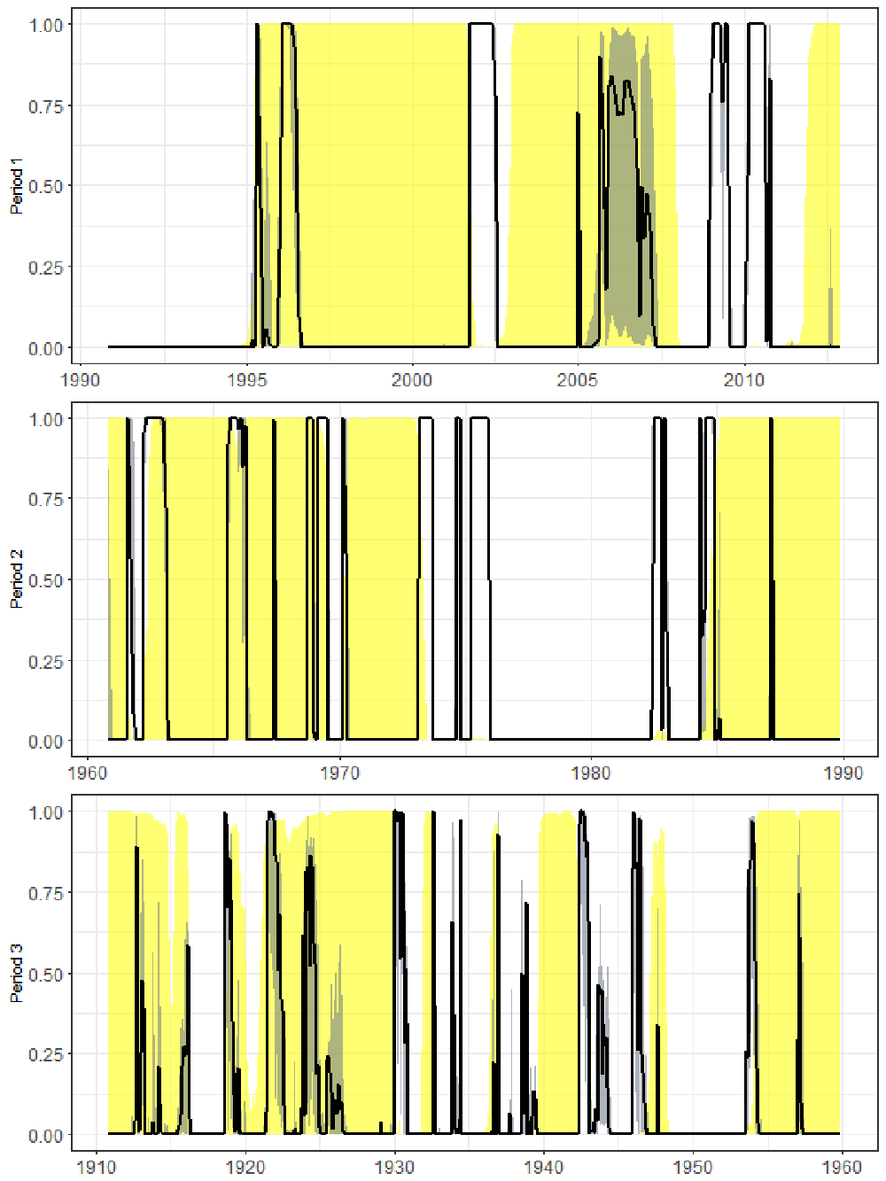
Note: The gray shaded region is the 90% pointwise confidence interval constructed by parametric bootstrap. The yellow shaded region is the probability of the boom regime estimated from the two-regime Markov switching model.
Confidence interval of . The fraction of the chartist, , is a nonlinear function of and . In principle we can construct the pointwise confidence interval by the delta method based on the asymptotic distribution of . However, it is difficult to interpret when the two-sided symmetric confidence interval goes beyond , which occurred in our experiment.
To avoid such difficulty, we can use the parametric bootstrap if we are willing to impose the normality assumption . Let be a bootstrap estimator where the superscript “” indexes the instance of bootstrap replication, and is the plug-in bootstrap estimator of the fraction. The parametric bootstrap is implemented as follows. We simulate a sequence where with . Given the data , we obtain the bootstrap estimator . Here we only bootstrap since the function only depends on the but not . After having , we plug it into and get . We repeat the bootstrap for 199 times, and compute the 5% and 95% sample quantiles of for each as the lower and upper bounds of the 90% two-sided pointwise confidence interval for .
The estimated pointwise bootstrap confidence interval is shown as the gray shaded region in Figure S5. The confidence interval is very narrow most of the time, in particular when is close to 0. Interestingly, along with the swings of the fraction of the chartists before the 2008 financial crisis, the uncertainty is manifest by the relatively wide confidence intervals.
S4 Implementation
S4.1 Gordon Growth Model
The original Gordon growth model is defined as where is the dividend at period , is the discount rate and is the average growth rate of dividends. Fama and French (2002) suggest that the Gordon growth model implies , where is the average dividend yield. We replace by and obtain
S4.2 Chartist-Only Model
Unlike the fundamentalist-only model, the chartist-only model is not a sub-model of the benchmark model, since cannot be set as 0. Even if we treat , or view the model as a sequence of models with , the three kernel-weighted moment functions still break down. When becomes arbitrarily small, the fundamental strategy will return infinitesimal profit. It violates the assumption that the fundamental strategy beats the chartist strategy under arbitrarily deviation from , and invalidates and , which were justified by arguing that the market is dominated by fundamentalists when occurs. Moreover, as a chartist ignores the fundamental value, is also unidentified; thus is not well defined.
Given the difficulty of adapting it to the chartist-only scenario, we slightly modify the benchmark model. In a market with only chartists, the demand equation becomes Notice that even without fundamentalists, the event remains well defined. Thus we introduce another kernel-weighted moment function
where is replaced by . This conditional moment is implied by the chartist-only model: when is close to 0, the return must also be small.
When estimating the chartist-only model, we utilize along with the five unconditional moment functions . The estimation involves six moments and two parameters , so that the -statistic still follows asymptotically under the null hypothesis.Extension of the Model
S5 Extension of the Model
Homogeneity and time invariance of the conditional variance in returns is restrictive, especially during a financial crisis. In this section, we discuss the possibility of relaxing this assumption.
We define to allow to vary across and . Similarly, define , which is time-varying but individual invariant as the chartist strategy does not consider any private signal. It follows that for the fundamental strategy , and for the chartist strategy . The investor chooses the fundamental strategy if , and the demand of the risky asset is
To compute the market aggregate demand, we need to specify the conditional variances since neither nor is observable from the data. A simple rule from the observed past history is an option for the chartist, while there is no consensus in the literature about the conditional variance of the fundamental strategy.
Consider imposing a parametric assumption on the joint distribution of , for example, jointly normal i.i.d. across time. This simple specification introduces two extra parameters: the variance of that captures the dispersion of the beliefs on the volatility, and the correlation coefficient between and . Although the theoretical model can be simulated by the method of simulated moments (MSM), all the closed-forms in the aggregate demand and the thin-set identification are lost. Such difficulty arises even before we study any dynamic specification in , which will incur additional parameters.
Analysis becomes more tractable if we assume that the distribution of and are independent. Let be the threshold such that . We solve to obtain
where . Define the lower bound and upper bound . As a result, the individual investment flow is
The probability of individual adopting the chartist strategy is , and the aggregate demand in the market is
| (S12) | |||||
If we further assume with being the proxy for , we can pointly identify under the event as in the main text. This identified will depend on the choice of . On the other hand, if we assume , where is the shock to each individual’s conditional variance independent of all other random variables, then the identification of remains under the event . Therefore, in this generalized model in which we allow time-varying and heterogeneous , we are able to pointly identify the same parameter as in the main text where a constant is assumed. As a result, the empirical estimates of in the three periods in the main text are informative about the magnitude of these parameters.
If we start with the general model, nevertheless, MSM will be necessary to handle the integrals and in the demand equation (S12). We do not have simple closed-forms for these integrals as , and all depend on and . Exploration of the conditional variance in this heterogeneous agent model would contribute to the theoretical modeling, asymptotic property of XMM-MSM, as well as the empirical findings. All these three aspects are new to the existing literature and they deserve thorough investigation in future research.
S6 Examples of Thin-Set Identification
Thin-set identification is not peculiar to our model. It is also useful for other heterogeneous agent models. Here we give two examples.
Example 1.
Lux (1995) formalizes herd behavior in speculative markets in which bubbles emerge as self-organizing process of infection among traders. Let be an index ranging from (extremely pessimistic) to (extremely optimistic). It characterizes the average opinion of speculative investors. The dynamics of is governed by the differential equation
where is a measure of the strength of herd behavior, and is a variable for the speed of change. The fraction of optimistic trader is (Lux, 1995, pp.884–885). When , the fraction of optimistic trader is 1.∎
Example 2.
He and Westerhoff (2005) analyze the creation of bull or bear market via nonlinear interactions between market participants—consumers, producers and heterogeneous speculators—in a behavioral commodity market model. They model the market share of chartists as , where is a switching parameter, is the long-run equilibrium price, and is the commodity price at time (He and Westerhoff, 2005, p.1582). When , the fraction of chartists is 1.∎