$\mathcal{G}$-SGD: Optimizing ReLU Neural Networks in its Positively Scale-Invariant Space

There have been some prior works that study the positively scale-invariant property of ReLU networks and design algorithms that are positively scale-invariant. For example, Badrinarayanan et al. (2015) notice the positive scale-invariance in ReLU netowrks, and inspired by this, they design algorithms to normalize gradients by layer-wise weight norm. Du et al. (2018) study the gradient flow in MLP or CNN models with linear, ReLU or Leaky ReLU activation, and prove the squared norms of gradient across different layers are automatically balanced and remained invariant in gradient descent with infinitesimal step size. In our work, we do not care whether the models are balanced or not. Besides, many other optimization algorithms also have positively scale-invariant property such as Newton’s method and natural gradient descent. The most related work is Path-SGD (Neyshabur et al., 2015), which also considers the geometry inspired by path norm. This work is different from ours: 1) they regularize the gradient in weight space by path norm while we optimize the loss function directly in a positively scale-invariant space; 2) they do not consider the dependency between paths and it’s hard for them to compute the exactly path-regularized gradients. Different from the previous works, we propose to directly optimize the ReLU networks in its positively scale-invariant space, instead of optimizing in the weight space which is not positive scale-invariant. To the best of our knowledge, at the first time, we solve this mismatch by theoretical analysis and an effective and efficient algorithm.

Let $N_{w}(x):\mathcal{X}\to\ \mathcal{Y}$ denote a $L$-layer multi-layer perceptron (MLP) with weight $w\in\mathcal{W}\subset\mathbb{R}^{m}$, the input space $\mathcal{X}\subset\mathbb{R}^{d}$ and the output space $\mathcal{Y}\subset\mathbb{R}^{K}$. In the $l$-th layer ($l=0,\cdots,L$), there are $h_{l}$ nodes. It is clear that, $h_{0}=d,h_{L}=K$. We denote the $i_{l}$-th node and its value as $O_{i_{l}}^{l}$ and $o_{i_{l}}^{l}$, respectively. We use $w^{l}$ to denote the weight matrix between layer $l-1$ and layer $l$, and use $w^{l}(i_{l-1},i_{l})$ to denote the weight connecting nodes $O^{l-1}_{i_{l-1}}$ and $O^{l}_{i_{l}}$. The values of the nodes are propagated as $o^{l}=\sigma((w^{l})^{T}o^{l-1})$, where $\sigma(\cdot)=max(\cdot,0)$ is the ReLU activation function. We use $(i_{0},\cdots,i_{L})$ to denote the path starting from input feature node $O_{i_{0}}^{0}$ to output node $O_{i_{L}}^{L}$ passing though hidden nodes $O^{1}_{i_{1}},\cdots,O^{L-1}_{i_{L-1}}$.

We can also regard the network structure as a directed graph $(\mathcal{O},E)$, where $\mathcal{O}=\{O_{1},\cdots,O_{H+d+K}\}$ is the set of nodes where $H$ denotes the number of hidden nodes and $E=\{e_{ij}\}$ denote the set of edges in a network where $e_{ij}$ denotes the edge pointing to $O_{j}$ from nodes $O_{i}$. We use $w_{e},e\in E$ to denote the weight on edge $e$. If $|E|=m$, the weights compose a vector $w=(w_{1},\cdots,w_{m})^{T}$. We define a path as a vector $p=(p_{1},\cdots,p_{m})^{T}$ and if the edge $e$ is contained in path $p$, $p_{e}=1$; otherwise $p_{e}=0$. Because a path crosses $L$ edges for an $L$-layer MLP, there are $L$ elements with value $1$ and others elements with value $0$. Using these notations, the value of path $p$ can be calculated as $v_{p}(w)=\prod_{i=1}^{m}w_{i}^{p_{i}}$ and the activation status of path $p$ can be calculated as $a_{p}(x;w)=\prod_{j:p_{e_{ij}}=1}\mathbb{I}(o_{j}(x;w)>0)$. We denote the set composed by all paths as $\mathcal{P}$ and the set composed by paths which contain edge connecting the $i_{0}$-th input node and the $k$-th output node as $\mathcal{P}^{i_{0},k}$. Thus, the output can be computed as follows:

We formally define the positive scaling operator. We first define a node positive scaling operator $g_{c,O}(w):\mathcal{W}\rightarrow\mathcal{W}$ with constant $c>0$ and one hidden node $O$ as

where $\tilde{w}^{l}(i_{l-1},i_{l})=c\cdot w^{l}(i_{l-1},i_{l})$ for $i_{l-1}=1,\cdots,h_{l-1}$; $\tilde{w}^{l+1}(i_{l},i_{l+1})=\frac{1}{c}\cdot w^{l+1}(i_{l},i_{l+1})$ for $i_{l+1}=1,\cdots,h_{l+1}$; and values of other elements of $\tilde{w}$ are the same with $w$.

We then collect all the $g_{(c_{1},\cdots,c_{H})}(\cdot)$ together to form a set $\mathcal{G}:=\{g_{(c_{1},\cdots,c_{H})}(\cdot):c_{1},\cdots,c_{H}\in\mathbb{R}^{+}\}$. It is easy to check that $\mathcal{G}$ together with the operation "$\circ$" is a group which is called positive scaling transformation group, and we call the group action of $\mathcal{G}$ on $\mathcal{W}$ as $\mathcal{G}$-action. (Please refer to Section 8 in Appendix.) Clearly, if there exists an operator $g\in\mathcal{G}$ to make $w=g(w^{\prime})$, ReLU networks $N_{w}$ and $N_{w^{\prime}}$ will generate the same output for any fixed input $x$. We define the positive scaling equivalence induced by $\mathcal{G}$-action.

Given $\mathcal{G}$-action on $\mathcal{W}$, the equivalence relation "$\sim_{\mathcal{G}}$" partitions $\mathcal{W}$ into $\mathcal{G}$-equivalent classes. The following theorem shows that the sufficient and necessary condition for ReLU networks in the same equivalent class is that they have the same values and activation status of paths.

Invariant variables for a group action are important and widely studied in group theory and geometry. We say a function $f:\mathcal{W}\rightarrow\mathbb{R}$ is invariant variable of $\mathcal{G}$-action if $f(w)=f(g(w)),\forall g\in\mathcal{G}$. Based on Theorem 3.3, a direct corollary is that values and activation status of paths are invariant variables under $\mathcal{G}$-action. Considering that 1) values of paths are $\mathcal{G}$-invariant variables while the weights aren’t; 2) values of paths together with the activation status determines an positive scale-equivalent class, and are sufficient to determine the loss, we propose to optimize the values of paths instead of weights.

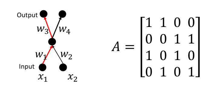
Although Theorem 3.3 shows the values of paths are invariant variables under $\mathcal{G}$-action, we find that the paths have inner-dependency and therefore their values and activation statuses are not independent. Let us consider the example in Figure 1. The values of paths have the relationship $v_{p^{4}}(w)=\frac{v_{p^{2}}(w)\cdot v_{p^{3}}(w)}{v_{p^{1}}(w)}$. Using the vector representation of paths that is described in section 2.2, we find that their path vectors follow the relationship $p^{4}=p^{2}+p^{3}-p^{1}$, which means that they are not linearly independent.

For a feedforward ReLU neural network, we suppose that $\mathcal{P}\subset\{0,1\}^{m}$ is the set composed by all path vectors. We denote the matrix composed by all paths as $A$ and call it structure matrix of ReLU networks. The size of $A$ is $m\times n$ where $n$ is the number of paths. We observe that the paths in matrix $A$ are not linearly independent. Then we study the rank of matrix $A$ and find a maximal linearly independent group of paths.

We design an algorithm called skeleton method to identify basis paths efficiently, which will be introduced in Section 4. For given values of basis paths and structure matrix, the values of $w$ can not be determined unless the values of free variables are fixed (Lay (1997)). Assume $w_{s_{1}},\cdots,w_{s_{H}}$ are selected to be the free variables which are called free skeleton weights, we prove that the activation status can be uniquely determined by the values of basis paths if signs of free skeleton weights are fixed. Thus, we have the following theorem which is a modification of Theorem 3.3.

The detailed proof of Theorem 3.4 and Theorem 3.6 are both depends on Lemma 9.1 in Appendix. In the following context, we always suppose that $\forall w\in\mathcal{W}$ have the same signs of free skeleton weights. According to Theorem 3.6 and the linear dependency between values of paths, the loss function can be calculated using values of basis paths if signs of free skeleton weights are fixed. We denote the the loss at training instance $(x,y)$ as $l(v;x,y)$ and propose to optimize the values of basis paths. Considering that values of basis paths are obtained through structure matrix $A$, the dimension of the space composed by values of basis paths should be equal to $rank(A)$. Then we define the following space.

We call the space composed by the values of basis paths $\mathcal{G}$-space, which is invariant under transformation group $\mathcal{G}$, i.e., it is composed by invariant variables under $\mathcal{G}$-action. Immediately, we can get the following corollary according to Theorem 3.6.

We measure the reduction of the dimension for positively scale-invariant space using the invariant ratio $H/m$, thus we can empirically test how severe this equivalence will influence the optimization in weight space.

Before the calculation of gradients in $\mathcal{G}$-space, we first design an algorithm called skeleton method to construct skeleton weights and basis paths for MLP whose depth is $L$ and width is $h$.

1. Construct skeleton weights: for weight matrix $w^{2},\cdots,w^{L-1}$, we select diagonal elements to be the skeleton weights. For weight matrix $w^{1}$, we select the element $w^{1}(i_{1}\mod d,i_{1})$ for column $i_{1}$ with $i_{1}=1,\cdots,h_{1}$ to be the skeleton weights. For weight matrix $w^{L}$, we select the element $w^{L}(i_{L-1},i_{L-1}\mod K)$ for row $i_{L-1}$ with $i_{L-1}=1,\cdots,h_{L-1}$ to be the skeleton weights. We call the rest weights non-skeleton weights. Figure 2 gives an illustration for skeleton weights in a MLP network.

2. Construct basis paths: A path which contains at most one non-skeleton weights is a basis path. The proof of this statement could be found in Appendix. For example, in Figure 2, the paths in red color and the paths with only one black weight are basis paths. Beyond that, the paths are non-basis paths.

Once we have basis paths, we can calculate the gradients w.r.t. basis path vector $v_{p^{i}}$, and iteratively update the model by

where $S^{t}$ is the mini-batch training data in iteration $t$. For the calculation of the gradients w.r.t. basis path vector, we introduce inverse-chain-rule method in next section.

The basic idea of the Inverse-Chain-Rule method is to connect the gradients w.r.t. weight vector and those w.r.t. basis path vector by exploring the chain rules in both directions. That is, we have,

We first compute the gradients w.r.t. weights, i.e., $\frac{\partial l(w;x,y)}{\partial w_{i}}$ for $i=1,\cdots,m$ using standard back propagation. Then we solve Eqn.(4.2) to obtain the gradients w.r.t. basis paths, i.e., $\frac{\partial l(v;x,y)}{\partial v_{j}}$ for $j=1,\cdots,m-H$. We denote matrix at the right side of Eqn.(4.2) as $G$. Given the following facts: (1) $\frac{\partial v_{p}}{\partial w_{e}}=\frac{v_{p}}{w_{e}}$ if the edge $e$ is contained in path $p$, otherwise 0; (2) according to the skeleton method, each non-skeleton weight will be contained in only one basis path, which means there is only one non-zero element in each column corresponding to non-skeleton weights in $G$, $G$ is sparse and thus the solution of Eqn.(4.2) is easy to obtain.

After the values of basis paths are updated by SGD, in a new iteration, we employ ICR again by leveraging BP with the new weight. Thus, we need to project the updates on basis paths back to the updates of weights.

We define the path-ratio of ${p^{j}}$ at iteration $t$ as $R^{t}({p^{j}}):=v_{p^{j}}^{t}/v_{p^{j}}^{t-1}$ and the weight-ratio of $w_{i}$ at iteration $t$ as $r^{t}(w_{i}):=w_{i}^{t}/w_{i}^{t-1}$. Assume that we have already obtained the path-ratio for all the basis paths $R^{t+1}({p^{j}})$ according to ICR method and the SGD update rule. Then we want to project the path-ratios onto the weight-ratios. We use the notation $\odot$ to denote the operation $w\odot p^{j}=\prod_{i=1}^{m}w_{i}^{p_{i}^{j}}$ Because we have $v_{p^{j}}(w)=w\odot p^{j}$, the weight-ratios obtained after the projection should satisfy the following relationship: $R^{t}(p^{j})=r^{t}(w)\odot p^{j}.$ Generalize the operator $\odot$ from vectors to matrices ²² 2 For strict description of operation ”$\odot$”, please refer to Section 8 in Appendix., we have the following relationship:

where the matrix $A^{\prime}=(p^{1},\cdots,p^{m-H})$. According to this relationship, we design Weight-Allocation Method to project the path-ratio to weight-ratio as described below. Suppose that $w_{1},\cdots,w_{H}$ are the free skeleton weights. We first add $H$ elements with value $1$ at the beginning in vector $(R^{t}(p^{1}),\cdots,R^{t}(p^{m-H}))$ to get a new $m$-dimensional vector. Then we append $H$ columns in matrix $A^{\prime}$ to get a new matrix $\tilde{A}$ as $\tilde{A}=[B,A^{\prime}]$ with $B=[I,\bf{0}]^{T}$ where $I$ is an $H\times H$ identity matrix with diagonal elements $1$ and $\bf{0}$ is an $H\times m$ zero matrix with all elements $0$. Then it is easy to prove that $rank(\tilde{A})=m$ and we have the following relationship:

We can get the weight-ratio by $\odot$ $\tilde{A}^{-1}$ on both sides of Eq.(7). Because we have $(r^{t}(w_{1}),\cdots,r^{t}(w_{m}))\odot\tilde{A}\odot\tilde{A}^{-1}=(r^{t}(w_{1}),\cdots,r^{t}(w_{m}))$ (refer to Section 8 in Appendix), we have

After the projection, we can see that weight-ratios of free skeleton weights equal $1$ which means that free skeleton weights will not be changed during the training process. According to the skeleton method again, $\tilde{A}$ is a sparse matrix and it is easy to calculate its inverse.

Actually, the projection method is not unique. Although we choose one special projection which fixed values of free skeleton weights in the Weight-Allocation method, we prove that different projection methods will results in the same updates in $\mathcal{G}$-space if they don’t change the signs of free skeleton weights.

Please note by combining the ICR and WA methods, we can obtain the explicit update rule for $\mathcal{G}$-SGD, which is concluded in Algorithm 1. In this way, we obtain the correct gradients. The extra computational complexity of the ICR and WA methods are far lower than that of forward and backward propagation, and can therefore be neglected in practice.

In this section, we apply our $\mathcal{G}$-SGD to image classification tasks and conduct experiments on CIFAR-10 and CIFAR-100 (Krizhevsky & Hinton, 2009). In our experiments, we employ the original ResNet architecture described in (He et al., 2016a). Specifically, there is no positive scaling invariance across residual blocks since the residual connections break down the structure matrix described in Section 3.2, we target the invariance in each residual block. For better comparison, we also conduct our studies on a stacked deep CNN described in He et al. (2016a) (refer to PlainNet), and target the positive scaling invariance across all layers. We train 34 layers ResNet and PlainNet models on the datasets following the training strategies in the original paper, and compare the performance between $\mathcal{G}$-SGD⁴⁴ 4 Batch normalization is widely used in modern CNN models. Please refer to Appendix for the combination of $\mathcal{G}$-SGD and batch normalization. and vanilla SGD algorithm. The detailed training strategies could be found in Appendix. In this section, we focus on the performance of different optimization algorithms, and will discuss the combination of $\mathcal{G}$-SGD and regularization in Appendix.

As shown in Figure 3 and Table 1, our $\mathcal{G}$-SGD clearly outperforms SGD on each network and each dataset. To be specific, 1) both the lowest training loss and best test accuracy are achieved by ResNet-34 with $\mathcal{G}$-SGD on both datasets, which indicates that $\mathcal{G}$-SGD indeed helps the optimization of ResNet model; 2) Since $\mathcal{G}$-SGD can eliminate the influence of positive scaling invariance across all layers of PlainNet, we observe the performance gain on PlainNet is larger than that on ResNet. For PlainNet model, $\mathcal{G}$-SGD surprisingly improves the accuracy numbers by 0.8 and 5.7 for CIFAR-10 and CIFAR-100, respectively, which verifies both the improper influence of positive scaling invariance for optimization in weight space and the benefit of optimization in $\mathcal{G}$ space. Moreover, Plain-34 trained by $\mathcal{G}$-SGD achieves even better accuracy than ResNet-34 trained by SGD on CIFAR-10, which shows the influence of invariance on optimization in weight space as well.

In this section, we study the influence of invariance on the optimization for ReLU Networks. As proved in Section 3, the dimension of weight space is larger than $\mathcal{G}$-space by $H$, where $H$ is the total number of the hidden nodes in a MLP or the feature maps in a CNN. We define the invariant ratio as $H/m$. We train several 2-hidden-layer MLP models on Fasion-MNIST (Xiao et al., 2017) with different number of hidden nodes in each layer, and analyze the performance gap $\Delta$ between the models optimized by $\mathcal{G}$-SGD and SGD. The detailed training strategies and network structures could be found in Appendix.

From Figure 4, we can see that, 1) for each number of $H$, $\mathcal{G}$-SGD clearly outperforms SGD on both training loss and test error, which verifies our claim that optimization loss function in $\mathcal{G}$ space is a better choice; 2) as $H$ increases, the invariant ratio decreases (because $m$ also increases for MLP) and $\Delta$ gradually decreases as well, which provides the evidence for that the positive scaling invariance in weight space indeed improperly influences the optimization.

In this section, we compare the performance of Path-SGD and that of $\mathcal{G}$-SGD. As described in Section 2.1, Path-SGD also consider the positive scaling invariance, but 1) instead of optimizing the loss function in $\mathcal{G}$-space, Path-SGD regularizes optimization by path norm; 2) Path-SGD ignores the dependency among the paths. We extend the experiments in Neyshabur et al. (2015) to $\mathcal{G}$-SGD without unbalance initialization, and conduct our studies on MNIST and CIFAR-10 datasets. The detailed training strategies and description of network structure can be found in Appendix.

As shown in Figure 5, while Path-SGD achieves better or equally good test accuracy and training loss than SGD for both MNIST and CIFAR10 datasets, $\mathcal{G}$-SGD achieves even better performance than Path-SGD, which is consistent with our theoretical analysis that considering the dependency between the paths and optimizing in $\mathcal{G}$-space bring benefit.

This work is partially supported by National Center for Mathematics and Interdisciplinary Sciences (NCMIS).

Theorem 3.3: Consider two ReLU neural networks with weights $w,w^{\prime}\in\mathcal{W}$. We have that $w\sim w^{\prime}$ iff for $\forall$ path $p$ and $\forall$ input $x\in\mathcal{X}$, we have $v_{p}(w)=v_{p}(w^{\prime})$ and $a_{p}(w,x)=a_{p}(w^{\prime},x)$.

Proof: For the necessity, if $w\sim w^{\prime}$, then there exist a positive scaling operator $g(\cdot)$ to make $g(w^{\prime})=w$. We use $i_{l}$ to denote the node index of nodes in layer-$l$ and $i_{l}\in[h_{l}]$. Then we have $w_{l}(i_{l-1},i_{l})=\frac{1}{c^{l-1}_{i_{l-1}}}\cdot c^{l}_{i_{l}}\cdot w^{\prime}_{l}(i_{l-1},i_{l})$ for $l=2,\cdots,L-1$, because each weight may be modified by the operators of its connected two nodes $g_{c^{l-1}_{i_{l-1}},O^{l-1}_{i_{l-1}}}$ and $g_{c^{l}_{i_{l}},O^{l}_{i_{l}}}$. Thus $v_{p}(w)=v_{p}(w^{\prime})$ is satisfied because

Next we need to prove that $a_{p}(w,x)=a_{p}(w^{\prime},x)$ is also satisfied. Because the value of the activation is determined by the sign of $o^{l},l=\{1,\cdots,L-1\}$, we just need to prove that

where $c^{l}_{i_{l}},i_{l}\in[h_{l}],l\in[L-1]$ are positive numbers. We prove it by induction.

(1) For $o^{1}$ of a $L$-layer MLP ($L>2$): Suppose that $\sigma(\cdot)$ is a ReLU activation function. For the $i_{1}$-th hidden node, we have

(2) For $o^{l}$ of the $L$-layer MLP ($l>2$): Suppose that

Then we have

Thus we finish the proof of necessity.

For the sufficiency, we need to prove that if $v_{p}(w)=v_{p}(w^{\prime})$ and $a_{p}(w,x)=a_{p}(w^{\prime},x)$ for $\forall$ path $p$ and $\forall$ input $x\in\mathcal{X}$, there exists $g\in\mathcal{G}$ to make $w^{\prime}=g(w)$. First, for hidden node $O_{i_{1}}^{1}$ in layer-1, we claim that their incoming weights satisfy the following relationship:

Because there exist path $p^{z_{1}},\cdots,p^{z_{h_{0}}}\in\mathcal{P}$ to make

and $v_{p}(w)=v_{p}(w^{\prime})$ for any $p$, we have

Then the claim is established. Then we prove each $c_{i_{1}}^{1}$ is positive. If there exist a constant $c_{i_{1}}^{1}$ is negative, then $o_{i_{1}}^{1}(w,x)\neq o_{i_{1}}^{1}(w^{\prime},x)$. If $o_{i_{l}}^{l}(w,x)>0$, we have $o_{i_{l}}^{l}(w^{\prime},x)=0$. Here we assume that $x\in\mathcal{X}$ where $\mathcal{X}$ is a compact set to make that $a_{p}(w,x)=a_{p}(w^{\prime},x),\forall p,\forall x$ is equivalent to $\textit{sgn}(o_{i_{l}}^{l}(w,x))=\textit{sgn}(o_{i_{l}}^{l}(w^{\prime},x)),\forall x,\forall l=1,\cdots,L$. Thus all the $c_{i_{1}}^{1}$ for $i_{1}=1,\cdots,h_{1}$ are positive. Then we use the operator $g_{c_{1}^{1},O_{1}^{1}}\circ\cdots\circ g_{c_{h_{1}}^{1},O_{h_{1}}^{1}}(w)$ to make the two networks with the same weights at layer 1. Then based on the networks with the same weights at layer 1, we gradually deal with the weights in other layers from layer 2 to the last layer using similar techniques as layer 1. We can finally construct $g\in\mathcal{G}$. Thus we finish the proof of the sufficiency.

$\Box$

In order to prove Theorem 3.4 and Theorem 3.6, we need to prove that there exist a group of paths which are independent and can represent other paths, and the activation status can be calculated using values of basis paths and signs of free skeleton weights. In order to simplify the proof, we leverage the basis paths constructed by skeleton method. We only show the proof of the following lemma, from which we can easily get Theorem 3.4 and Theorem 3.6.

Proof sketch: Let us consider the matrix $A^{\prime}=(p^{1},\cdots,p^{m-H})$ composed by basis paths constructed by skeleton method:

There is an identity matrix with size $z\times z$ where $z$ is the number of skip skeleton paths. This identity matrix means that $w_{i}$ is a non-skeleton weight and is contained in $p^{i}$, $i\leq z$. Thus, through the row transformation of the matrix, $B_{1}$ can be transformed to zero matrix. According to skeleton method, column vectors in $B_{2}$ are independent because skeleton weight will only appear in one all-basis path. Thus the independent property has been proved. Furthermore, by leveraging the structure of matrix $A^{\prime}$, it is easily to check that for a non-skeleton path $p$, it can be calculated as $p=\sum_{i=1}^{z}\alpha_{i}p^{i}-\sum_{j=z+1}^{m-H}\alpha_{j}p^{j}$ where $\alpha_{i}=0$ or $1$ and $\alpha_{j}=0,1,2\cdots,L-1$. More specifically, if $p$ contains $w_{i}$, $i\leq z$, then $\alpha_{i}=1$; otherwise, $\alpha_{i}=0$.

References

- Badrinarayanan et al. (2015) Vijay Badrinarayanan, Bamdev Mishra, and Roberto Cipolla. Symmetry-invariant optimization in deep networks. arXiv preprint arXiv:1511.01754, 2015.
- Cheng et al. (2016) Heng-Tze Cheng, Levent Koc, Jeremiah Harmsen, Tal Shaked, Tushar Chandra, Hrishi Aradhye, Glen Anderson, Greg Corrado, Wei Chai, Mustafa Ispir, et al. Wide & deep learning for recommender systems. In Proceedings of the 1st Workshop on Deep Learning for Recommender Systems, pp. 7–10. ACM, 2016.
- Du et al. (2018) Simon S Du, Wei Hu, and Jason D Lee. Algorithmic regularization in learning deep homogeneous models: Layers are automatically balanced. Advances in Neural Information Processing Systems, 2018.
- Hahnloser et al. (2000) Richard HR Hahnloser, Rahul Sarpeshkar, Misha A Mahowald, Rodney J Douglas, and H Sebastian Seung. Digital selection and analogue amplification coexist in a cortex-inspired silicon circuit. Nature, 405(6789):947, 2000.
- He et al. (2015) Kaiming He, Xiangyu Zhang, Shaoqing Ren, and Jian Sun. Delving deep into rectifiers: Surpassing human-level performance on imagenet classification. In Proceedings of the IEEE international conference on computer vision, pp. 1026–1034, 2015.
- He et al. (2016a) Kaiming He, Xiangyu Zhang, Shaoqing Ren, and Jian Sun. Deep residual learning for image recognition. In Proceedings of the IEEE conference on computer vision and pattern recognition, pp. 770–778, 2016a.
- He et al. (2016b) Kaiming He, Xiangyu Zhang, Shaoqing Ren, and Jian Sun. Identity mappings in deep residual networks. In European conference on computer vision, pp. 630–645. Springer, 2016b.
- Huang et al. (2017) Gao Huang, Zhuang Liu, Laurens Van Der Maaten, and Kilian Q Weinberger. Densely connected convolutional networks. In CVPR, volume 1, pp. 3, 2017.
- Krizhevsky & Hinton (2009) Alex Krizhevsky and Geoffrey Hinton. Learning multiple layers of features from tiny images. CIFAR, 2009.
- Lay (1997) David C Lay. Linear Algebra and its applications, 1997. Addison Wesley Longman, Inc. ISBN 0-201-76717-1, 1997.
- LeCun et al. (2015) Yann LeCun, Yoshua Bengio, and Geoffrey Hinton. Deep learning. Nature, 521(7553):436–444, 2015.
- Neyshabur et al. (2015) Behnam Neyshabur, Ruslan R Salakhutdinov, and Nati Srebro. Path-sgd: Path-normalized optimization in deep neural networks. In Advances in Neural Information Processing Systems, pp. 2422–2430, 2015.
- Rumelhart et al. (1986) David E Rumelhart, Geoffrey E Hinton, and Ronald J Williams. Learning representations by back-propagating errors. nature, 323(6088):533, 1986.
- Vaswani et al. (2017) Ashish Vaswani, Noam Shazeer, Niki Parmar, Jakob Uszkoreit, Llion Jones, Aidan N Gomez, Łukasz Kaiser, and Illia Polosukhin. Attention is all you need. In Advances in Neural Information Processing Systems, pp. 5998–6008, 2017.
- Wang et al. (2017) Ruoxi Wang, Bin Fu, Gang Fu, and Mingliang Wang. Deep & cross network for ad click predictions. In Proceedings of the ADKDD’17, pp. 12. ACM, 2017.
- Xiao et al. (2017) Han Xiao, Kashif Rasul, and Roland Vollgraf. Fashion-mnist: a novel image dataset for benchmarking machine learning algorithms. 2017.
- Zagoruyko & Komodakis (2016) Sergey Zagoruyko and Nikos Komodakis. Wide residual networks. arXiv preprint arXiv:1605.07146, 2016.
- Zheng et al. (2018) Shuxin Zheng, Qi Meng, Huishuai Zhang, Wei Chen, Nenghai Yu, and Tie-Yan Liu. Capacity control of relu neural networks by basis-path norm. arXiv preprint arXiv:1809.07122, 2018.
Appendix: -SGD: Optimizing ReLU Neural Networks in its Positively Scale-Invariant space
The Appendix document is composed of examples of skeleton weights and basis paths for different MLP structures, proofs of propositions, lemmas and theorems and the additional information about the experiments in the paper Optimization of ReLU Neural Networks using -Stochastic Gradient Descent .