跳到论文正文
W Papers独立论文阅读器 arXiv:1802.03687 论文正文 计算阅读时间 · 0%
引用这篇论文根据当前论文元数据生成,正式投稿前建议核对。


License: arXiv.org perpetual non-exclusive license
arXiv:1802.03687v1 [math.NA] 11 Feb 2018

Computation of Transmission Eigenvalues for Elastic WavesThanks: The research of X. Ji is partially supported by the National Natural Science Foundation of China with Grant Nos. 11271018 and 91630313, and National Center for Mathematics and Interdisciplinary Sciences, Chinese Academy of Sciences. The research of P. Li was supported in part by the NSF grant DMS-1151308. The research of J. Sun was supported in part by the NSF grant DMS-1521555.

Xia Ji Address: LSEC, Academy of Mathematics and System Sciences, Chinese Academy of Sciences, Beijing, 100190, China. Email address: jixia@lsec.cc.ac.cn , Peijun Li Address: Department of Mathematics, Purdue University, West Lafayette, IN 47907, USA. Email address: lipeijun@math.purdue.edu and Jiguang Sun Address: Department of Mathematical Sciences, Michigan Technological University, Houghton, MI 49931, USA. Email address: jiguangs@mtu.edu
Abstract.

The goal of this paper is to develop numerical methods computing a few smallest elasticity transmission eigenvalues, which are of practical importance in inverse scattering theory. The problem is challenging since it is nonlinear, non-self-adjoint, and of fourth order. We construct a nonlinear function whose values are generalized eigenvalues of a series of self-adjoint fourth order problems. The roots of the function are the transmission eigenvalues. Using an H2H^{2}-conforming finite element for the self-adjoint fourth order eigenvalue problems, we employ a secant method to compute the roots of the nonlinear function. The convergence of the proposed method is proved. In addition, a mixed finite element method is developed for the purpose of verification. Numerical examples are presented to verify the theory and demonstrate the effectiveness of the two methods.

Key words and phrases: 
Transmission eigenvalue problem, elastic wave equation, finite element method
2000 Mathematics Subject Classification
65N25, 65N30, 47B07

1. Introduction

Transmission eigenvalues have important applications in inverse scattering theory. For example, they can be used to obtain useful information on the physical properties of the scattering targets [8, 25]. In this paper, we consider the interior transmission eigenvalue problem for elastic waves. Similar to the cases of acoustic and electromagnetic waves, the elasticity transmission eigenvalue (ETE) problem plays a critical role in the qualitative reconstruction methods for inhomogeneous media. There are only a few theoretical studies on the ETE problem [10, 11, 4, 3]. It is shown in [3] that there exists a countable set of elasticity transmission eigenvalues under suitable conditions on elastic tensors and mass densities.

Numerical methods for the acoustic transmission eigenvalues have been developed by many researchers recently [12, 24, 21, 1, 19, 22, 9, 20, 28]. However, there exist much fewer papers [23, 26, 16] for the electromagnetic transmission eigenvalue problems. It is highly non-trivial to develop finite element methods for the transmission eigenvalue problems in general since the problem is nonlinear and nonself-adjoint [27]. Although out of the scope of the current paper, it is useful to point out that the finite element discretization usually leads to non-Hermitian matrix eigenvalue problems. It is challenging to compute (interior) generalized eigenvalues for non-Hermitian matrices. In particular, when the size of matrices is large and there is no spectrum information, classical methods in numerical linear algebra would fail. New methods have emerged to treat such difficult problems [17, 18].

The goal of this paper is to develop effective numerical methods to compute a few smallest real transmission eigenvalues, which can be used to estimate material property of the elastic body (see, e.g., [25]). Unlike the classical Laplacian eigenvalue problem or the biharmonic eigenvalue problem, the transmission eigenvalue problem is nonlinear and nonself-adjoint. To overcome this issue, we reformulate the problem as a combination of a nonlinear function and a series of fourth order self-adjoint eigenvalue problems. Specifically, the ETE is first written as a nonlinear fourth order problem, which turns out to be a quadratic eigenvalue problem. To avoid dealing with the nonself-adjointness directly, we construct a nonlinear function whose roots are the elasticity transmission eigenvalues. The values of the nonlinear function are generalized eigenvalues of self-adjoint coercive fourth order problems, which can be treated using classical H2H^{2}-conforming finite elements. A secant based iterative method is adopted to compute the roots of the nonlinear function. In addition, we give a mixed method using the Lagrange elements for the purpose of verification.

The current paper, to the authors’ knowledge, is the first numerical study on the ETE. We hope that it can attract more numerical analysts to this interesting and challenging topic. The rest of the paper is organized as follows. In Section 2, we introduce the elasticity transmission eigenvalue problem and derive a quadratic eigenvalue problem based on a fourth order partial differential equation. To avoid direct treatment of the nonlinearity and nonself-adjointness, the problem is decomposed into a nonlinear function and a series of related linear self-adjoint fourth order eigenvalue problems. The values of the nonlinear function are generalized eigenvalues of the fourth order problems. The roots of the nonlinear function are transmission eigenvalues. H2H^{2}-conforming Argyris element for the fourth order problems is presented in Section 3. A secant based iterative method is used in Section 4 to compute roots of the nonlinear function. Section 5 introduces a mixed finite element method for verification. Numerical experiments are presented in Section 6. The paper is concluded with some discussion and future works in Section 7.

2. The elasticity transmission eigenvalue problem

Let 𝒙=(x,y)⊤∈ℝ2\boldsymbol{x}=(x,y)^{\top}\in\mathbb{R}^{2} and D⊂ℝ2D\subset\mathbb{R}^{2} be a bounded Lipschitz domain. Consider the two-dimensional elastic wave problem of finding 𝒖\boldsymbol{u} with zero trace on the boundary of DD, i.e., Γ\Gamma, such that

(2.1) ∇⋅σ⁡(𝒖)+ω2​ρ​𝒖=𝟎in​D⊂ℝ2,\nabla\cdot\sigma(\boldsymbol{u})+\omega^{2}\rho\boldsymbol{u}={\boldsymbol{0}}\quad\text{in}~D\subset\mathbb{R}^{2},

where 𝒖⁡(𝒙)=(u1​(𝒙),u2​(𝒙))⊤\boldsymbol{u}(\boldsymbol{x})=(u_{1}(\boldsymbol{x}),u_{2}(\boldsymbol{x}))^{\top} is the displacement vector of the wave field, ω>0\omega>0 is the angular frequency, ρ\rho is the mass density, and σ⁡(𝒖)\sigma(\boldsymbol{u}) is the stress tensor given by the generalized Hooke law

σ⁡(𝒖)=2​μ​ε​(𝒖)+λ​tr​(ε⁡(𝒖))​I.\sigma(\boldsymbol{u})=2\mu\varepsilon(\boldsymbol{u})+\lambda{\rm tr}(\varepsilon(\boldsymbol{u})){\rm I}.

Here the strain tensor ε⁡(𝒖)\varepsilon(\boldsymbol{u}) is given by

ε⁡(𝒖)=12​(∇𝒖+(∇𝒖)⊤),\varepsilon(\boldsymbol{u})=\frac{1}{2}(\nabla\boldsymbol{u}+(\nabla\boldsymbol{u})^{\top}),

where the two constants μ,λ\mu,\lambda are called the Lamé parameters satisfying μ>0,λ+μ>0\mu>0,\lambda+\mu>0, I∈ℝ2×2{\rm I}\in\mathbb{R}^{2\times 2} is the identity matrix, and ∇𝒖\nabla\boldsymbol{u} is the displacement gradient tensor

∇𝒖=[∂xu1∂yu1∂xu2∂yu2].\nabla\boldsymbol{u}=\begin{bmatrix}\partial_{x}u_{1}&\partial_{y}u_{1}\\ \partial_{x}u_{2}&\partial_{y}u_{2}\end{bmatrix}.

Explicitly, we have

(2.2) σ⁡(𝒖)=[(λ+2​μ)​∂xu1+λ​∂yu2μ⁡(∂yu1+∂xu2)μ⁡(∂xu2+∂yu1)λ​∂xu1+(λ+2​μ)​∂yu2].\sigma(\boldsymbol{u})=\begin{bmatrix}(\lambda+2\mu)\partial_{x}u_{1}+\lambda\partial_{y}u_{2}&\mu(\partial_{y}u_{1}+\partial_{x}u_{2})\\ \mu(\partial_{x}u_{2}+\partial_{y}u_{1})&\lambda\partial_{x}u_{1}+(\lambda+2\mu)\partial_{y}u_{2}\end{bmatrix}.

Given 𝒖,𝒗∈H01​(D)2{\boldsymbol{u}},{\boldsymbol{v}}\in H_{0}^{1}(D)^{2}, it follows from the integration by parts that

(2.3) (σ⁡(𝒖),∇𝒗)=∫Dσ⁡(𝒖):∇𝒗​𝑑𝒙=∫D(2​μ​ε​(𝒖):ε⁡(𝒗)+λ⁡(∇⋅𝒖)​(∇⋅𝒗))​𝑑𝒙,({\sigma}({\boldsymbol{u}}),\nabla{\boldsymbol{v}})=\int_{D}\sigma(\boldsymbol{u}):\nabla\boldsymbol{v}\,{\rm d}\boldsymbol{x}=\int_{D}\left(2\mu\varepsilon({\boldsymbol{u}}):\varepsilon({\boldsymbol{v}})+\lambda(\nabla\cdot{\boldsymbol{u}})(\nabla\cdot{\boldsymbol{v}})\right){\rm d}{\boldsymbol{x}},

where A:B=tr⁡(A​B⊤)A:B={\rm tr}(AB^{\top}) is the Frobenius inner product of square matrices AA and BB. We recall the first Korn inequality [5, Corollary 11.2.25]: there exists a positive constant CC such that

‖ε⁡(𝒖)‖L2≥C​‖𝒖‖H1for all ​𝒖∈H01​(D)2,\|\varepsilon({\boldsymbol{u}})\|_{L^{2}}\geq C\|{\boldsymbol{u}}\|_{H^{1}}\quad\text{for all }{\boldsymbol{u}}\in H_{0}^{1}(D)^{2},

which guarantees the well-posedness of (2.3).

Let μ0,λ0\mu_{0},\lambda_{0} be the Lamé parameters of the free space. Assume the domain DD is filled with a homogeneous and isotropic elastic medium with Lamé constants λ1\lambda_{1} and μ1\mu_{1}. The transmission eigenvalue problem for the elastic waves is to find values of ω2\omega^{2} such that there exists non-trivial solutions 𝒖,𝒗\boldsymbol{u},\boldsymbol{v} satisfying

(2.4a) ∇⋅σ0​(𝒖)+ω2​ρ0​𝒖=0\displaystyle\nabla\cdot\sigma_{0}(\boldsymbol{u})+\omega^{2}\rho_{0}\boldsymbol{u}=0 in​D,\displaystyle\quad\text{in}~D,
(2.4b) ∇⋅σ1​(𝒗)+ω2​ρ1​𝒗=0\displaystyle\nabla\cdot\sigma_{1}(\boldsymbol{v})+\omega^{2}\rho_{1}\boldsymbol{v}=0 in​D,\displaystyle\quad\text{in}~D,
(2.4c) 𝒖=𝒗\displaystyle\boldsymbol{u}=\boldsymbol{v} on​Γ,\displaystyle\quad\text{on}~\Gamma,
(2.4d) σ0​(𝒖)​𝝂=σ1​(𝒗)​𝝂\displaystyle\sigma_{0}(\boldsymbol{u}){\boldsymbol{\nu}}=\sigma_{1}(\boldsymbol{v}){\boldsymbol{\nu}} on​Γ,\displaystyle\quad\text{on}~\Gamma,

where

σi(𝒖)=[(λi+2​μi)​∂xu1+λi​∂yu2μi​(∂yu1+∂xu2)μi​(∂xu2+∂yu1)λi​∂xu1+(λi+2​μi)​∂yu2],i=0,1,\sigma_{i}(\boldsymbol{u})=\begin{bmatrix}(\lambda_{i}+2\mu_{i})\partial_{x}u_{1}+\lambda_{i}\partial_{y}u_{2}&\mu_{i}(\partial_{y}u_{1}+\partial_{x}u_{2})\\ \mu_{i}(\partial_{x}u_{2}+\partial_{y}u_{1})&\lambda_{i}\partial_{x}u_{1}+(\lambda_{i}+2\mu_{i})\partial_{y}u_{2}\end{bmatrix},\quad i=0,1,

and σ​𝝂\sigma{\boldsymbol{\nu}} denotes the matrix multiplication of the stress tensor σ\sigma and the normal vector 𝝂\boldsymbol{\nu}.

In this paper, we consider the case when ρ0≠ρ1,σ0=σ1=σ\rho_{0}\neq\rho_{1},\sigma_{0}=\sigma_{1}=\sigma, i.e., the case of equal elastic tensors [3]. In addition, we assume that the mass density distributions satisfy the following conditions

(2.5) p≤ρ0​(𝒙)≤P,p∗≤ρ1​(𝒙)≤P∗,𝒙∈D,p\leq\rho_{0}({\boldsymbol{x}})\leq P,\quad p_{*}\leq\rho_{1}({\boldsymbol{x}})\leq P_{*},\quad{\boldsymbol{x}}\in D,

where p,p∗p,p_{*} and P,P∗P,P_{*} are positive constants.

Define the Sobolev space

(2.6) V={ϕ∈H2(D)2:ϕ=𝟎 and σ(ϕ)𝝂=𝟎onΓ}.V=\{\boldsymbol{\phi}\in H^{2}(D)^{2}:{\boldsymbol{\phi}}={\boldsymbol{0}}\text{ and }\sigma({\boldsymbol{\phi}}){\boldsymbol{\nu}}={\bf 0}~\text{on}~\Gamma\}.

Let 𝒘=𝒖−𝒗{\boldsymbol{w}}={\boldsymbol{u}}-{\boldsymbol{v}}. The transmission eigenvalue problem can be formulated as follows: Find ω2\omega^{2} and 𝒘≠𝟎{\boldsymbol{w}}\neq{\bf 0} such that

(2.7) (∇⋅𝝈+ω2​ρ1)​(ρ1−ρ0)−1​(∇⋅𝝈+ω2​ρ0)​𝒘=𝟎.\left(\nabla\cdot{\boldsymbol{\sigma}}+\omega^{2}\rho_{1}\right)(\rho_{1}-\rho_{0})^{-1}\left(\nabla\cdot{\boldsymbol{\sigma}}+\omega^{2}\rho_{0}\right){\boldsymbol{w}}={\bf 0}.

The corresponding weak formulation of (2.7) is to find ω2∈ℂ\omega^{2}\in\mathbb{C} and 𝟎≠𝒘∈V{\bf 0}\neq{\boldsymbol{w}}\in V such that

(2.8) ((ρ1−ρ0)−1​(∇⋅σ+ω2​ρ0)​𝒘,(∇⋅σ+ω2​ρ1)​𝝋)=𝟎for all ​𝝋∈V.\left((\rho_{1}-\rho_{0})^{-1}\left(\nabla\cdot{\sigma}+\omega^{2}\rho_{0}\right){\boldsymbol{w}},\left(\nabla\cdot{\sigma}+\omega^{2}\rho_{1}\right){\boldsymbol{\varphi}}\right)={\bf 0}\quad\text{for all }{\boldsymbol{\varphi}}\in V.

Let τ=ω2\tau=\omega^{2}. We define two sesquilinear forms on V×VV\times V

𝒜τ​(ϕ,𝝋)\displaystyle\mathcal{A}_{\tau}({\boldsymbol{\phi}},{\boldsymbol{\varphi}}) =((ρ1−ρ0)−1​(∇⋅σ+τ​ρ0)​ϕ,(∇⋅σ+τ​ρ0)​𝝋)+τ2​(ρ0​ϕ,𝝋),\displaystyle=\left((\rho_{1}-\rho_{0})^{-1}\left(\nabla\cdot{\sigma}+\tau\rho_{0}\right){\boldsymbol{\phi}},\left(\nabla\cdot{\sigma}+\tau\rho_{0}\right){\boldsymbol{\varphi}}\right)+\tau^{2}(\rho_{0}{\boldsymbol{\phi}},{\boldsymbol{\varphi}}),
ℬ⁡(ϕ,𝝋)\displaystyle\mathcal{B}({\boldsymbol{\phi}},{\boldsymbol{\varphi}}) =(σ⁡(ϕ),∇𝝋).\displaystyle=({\sigma}({\boldsymbol{\phi}}),\nabla{\boldsymbol{\varphi}}).

It is clear that 𝒜τ\mathcal{A}_{\tau} is symmetric. Due to (2.3), ℬ\mathcal{B} is also symmetric.

The variational problem (2.8) can be written equivalently as follows: Find τ∈ℂ\tau\in\mathbb{C} and 𝟎≠𝒘∈V{\bf 0}\neq{\boldsymbol{w}}\in V such that

(2.9) 𝒜τ​(𝒘,𝝋)=τ​ℬ​(𝒘,𝝋)for all ​𝝋∈V.\mathcal{A}_{\tau}({\boldsymbol{w}},{\boldsymbol{\varphi}})=\tau\mathcal{B}({\boldsymbol{w}},{\boldsymbol{\varphi}})\quad\text{for all }{\boldsymbol{\varphi}}\in V.

This is a nonlinear problem since τ\tau appears on both sides of the equation. For a fixed τ\tau, we consider an associated generalized eigenvalue problem

(2.10) 𝒜τ​(𝒘,𝝋)=γ⁡(τ)​ℬ​(𝒘,𝝋)for all ​𝝋∈V.\mathcal{A}_{\tau}({\boldsymbol{w}},{\boldsymbol{\varphi}})=\gamma(\tau)\mathcal{B}({\boldsymbol{w}},{\boldsymbol{\varphi}})\quad\text{for all }{\boldsymbol{\varphi}}\in V.

Formally, τ\tau is a transmission eigenvalue if τ\tau is a root of the nonlinear function

(2.11) f⁡(τ):=γ⁡(τ)−τ.f(\tau):=\gamma(\tau)-\tau.

In the rest of this section, we study the generalized eigenvalue problem (2.10). It is shown in [15] that there exists β>0\beta>0 such that

‖∇⋅σ⁡(ϕ)‖2+‖ϕ‖2≥β​‖ϕ‖H2​(D)22for ​ϕ∈V.\|\nabla\cdot{\sigma}({\boldsymbol{\phi}})\|^{2}+\|{\boldsymbol{\phi}}\|^{2}\geq\beta\|{\boldsymbol{\phi}}\|^{2}_{H^{2}(D)^{2}}\quad\text{for }{\boldsymbol{\phi}}\in V.

The following lemma is useful in the subsequent analysis. The proof can be found in [3].

Lemma 2.1.

Assume that p∗≥1≥Pp_{*}\geq 1\geq P. Then 𝒜τ\mathcal{A}_{\tau} is a coercive sesquilinear form on V×VV\times V, i.e., there exists a constant α>0\alpha>0 such that

𝒜τ​(ϕ,ϕ)≥α​‖ϕ‖2for all ​ϕ∈V.\mathcal{A}_{\tau}({\boldsymbol{\phi}},{\boldsymbol{\phi}})\geq\alpha\|{\boldsymbol{\phi}}\|^{2}\quad\text{for all }{\boldsymbol{\phi}}\in V.

The source problem associated with (2.10) is to find 𝒖∈V{\boldsymbol{u}}\in V such that, for 𝒇∈H1​(D)2{\boldsymbol{f}}\in H^{1}(D)^{2},

(2.12) 𝒜τ​(𝒖,ϕ)=(σ⁡(𝒇),∇ϕ)for all ​ϕ∈V.\mathcal{A}_{\tau}({\boldsymbol{u}},{\boldsymbol{\phi}})=(\sigma({\boldsymbol{f}}),\nabla{\boldsymbol{\phi}})\quad\text{for all }{\boldsymbol{\phi}}\in V.

The following theorem is a direct consequence of the Lax–Milgram Lemma.

Theorem 2.2.

There exists a unique solution 𝐮∈V{\boldsymbol{u}}\in V to (2.12). Furthermore, it holds that

(2.13) ‖𝒖‖H2​(D)2≤C​‖𝒇‖H1​(D)2.\|{\boldsymbol{u}}\|_{H^{2}(D)^{2}}\leq C\|{\boldsymbol{f}}\|_{H^{1}(D)^{2}}.
Proof.

It is easy to show that 𝒜τ\mathcal{A}_{\tau} is bounded. The coercivity of 𝒜τ\mathcal{A}_{\tau} follows Lemma 2.1. Let FF be a linear functional on VV such that

F⁡(ϕ):=(σ⁡(𝒇),∇ϕ),F({\boldsymbol{\phi}}):=(\sigma({\boldsymbol{f}}),\nabla{\boldsymbol{\phi}}),

for all ϕ∈V{\boldsymbol{\phi}}\in V. Then the Lax-Milgram Lemma implies that there exists a unique solution 𝒖{\boldsymbol{u}} to the problem

𝒜τ​(𝒖,ϕ)=F⁡(ϕ)for all ​ϕ∈V.\mathcal{A}_{\tau}({\boldsymbol{u}},{\boldsymbol{\phi}})=F({\boldsymbol{\phi}})\quad\text{for all }{\boldsymbol{\phi}}\in V.

Moreover, we have

‖𝒖‖H2​(D)2≤C​‖F‖V′,\|{\boldsymbol{u}}\|_{H^{2}(D)^{2}}\leq C\|F\|_{V^{\prime}},

where V′V^{\prime} represents the dual space of VV. Following from the definition of σ⁡(𝒇)\sigma({\boldsymbol{f}}), we obtain from a simple calculation that

‖F‖V′≤Cλ,μ​‖𝒇‖H1​(D)2,\|F\|_{V^{\prime}}\leq C_{\lambda,\mu}\|{\boldsymbol{f}}\|_{H^{1}(D)^{2}},

which shows the estimate (2.13) and completes the proof. ∎

Remark 2.3.

In the rest of the paper, we assume that the following regularity for 𝐮{\boldsymbol{u}} holds

(2.14) ‖𝒖‖H2+ξ​(Ω)2≤C​‖𝒇‖H1​(D)2.\|{\boldsymbol{u}}\|_{H^{2+\xi}(\Omega)^{2}}\leq C\|{\boldsymbol{f}}\|_{H^{1}(D)^{2}}.

Note that a similar regularity holds for the biharmonic equation [6, 14, 7] where the elliptic regularity ξ∈(12,1]\xi\in(\frac{1}{2},1] is determined by the angles at the corners of DD and ξ=1\xi=1 if DD is convex.

It follows from Theorem 2.2 that there exists a solution operator T:H1​(D)2→VT:H^{1}(D)^{2}\to V such that

𝒖=T​𝒇.{\boldsymbol{u}}=T{\boldsymbol{f}}.

Clearly, the operator TT is self-adjoint since 𝒜τ\mathcal{A}_{\tau} is symmetric; TT is also a compact operator due to the compact embedding of H2​(D)2H^{2}(D)^{2} into H1​(D)2H^{1}(D)^{2} (see, e.g., Theorem 1.2.1 of [27]). The generalized eigenvalue problem (2.10) has the following equivalent operator form

𝒖=η​T​𝒖,where ​η=γ−1.{\boldsymbol{u}}=\eta T{\boldsymbol{u}},\quad\text{where }\eta=\gamma^{-1}.

From classical spectral theory of compact self-adjoint operators, i.e., the Hilbert-Schmidt theory, TT has at most a countable set of real eigenvalues and 00 is the only possible accumulation point. Consequently, we have the following lemma for the generalized eigenvalue value problem (2.10).

Lemma 2.4.

Let ρ0\rho_{0} and ρ1\rho_{1} satisfy (2.5) such that the condition in Lemma (2.1) is fulfilled. Then the generalized eigenvalue value problem (2.10) has at most a countable set of positive eigenvalues and +∞+\infty is the only possible accumulation point.

Roughly speaking, to compute real transmission eigenvalues, one needs to computes the roots of the nonlinear function ff. The values of f⁡(τ)f(\tau) are generalized eigenvalues of (2.10), which is approximated by the H2H^{2}-conforming Argyris element.

3. A conforming finite element method

In this section, we propose a conforming finite element for (2.10). The convergence of the source problem (2.12) is established first. The theory of Babuška and Osborn [2] is then applied to obtain the convergence of the eigenvalue problem (2.10).

Let 𝒯\mathcal{T} be a regular triangular mesh for DD and K∈𝒯K\in\mathcal{T} be a triangle. We employ the H2H^{2}-conforming Argyris element, which uses 𝒫5\mathcal{P}_{5} - the set of polynomials of degree up to 55 on KK, to discretize (2.10). Note that dim​(𝒫5)=21\text{dim}(\mathcal{P}_{5})=21. For 𝒩={N1,…,N21}\mathcal{N}=\{N_{1},\ldots,N_{21}\}, 33 degrees of freedom are the values at the vertices of KK, 66 degrees of freedom are the values of the first order partial derivatives at the vertices of KK, 99 degrees of freedoms are the values of the second order derivatives at the vertices of KK, and 33 degrees of freedom are the values of the normal derivatives at the midpoints of three edges of KK [5].

Note that the Argyris element does not belong to the affine families. This is due to the fact that normal derivatives are used as degrees of freedom. Fortunately, their interpolation properties are quite similar to those of affine families. Hence the Argyris element is referred to be almost-affine element. Let v∈H2​(D)v\in H^{2}(D) and Ih​vI_{h}v be the interpolation of vv by the Argyris element. For v∈H1+α​(D)v\in H^{1+\alpha}(D), α>0\alpha>0, the following interpolation result holds (see, e.g., [13])

(3.1) ‖v−Ih​v‖H2​(D)≤C​hs−1​|v|Hs+1​(D),\|v-I_{h}v\|_{H^{2}(D)}\leq Ch^{s-1}|v|_{H^{s+1}(D)},

where 1≤s≤min⁡{5,1+α}1\leq s\leq\min\{5,1+\alpha\} depending regularity of vv.

Let VhV_{h} be the Argyris finite element space associated with 𝒯\mathcal{T}. The discrete problem for (2.12) is to find 𝒖h∈Vh{\boldsymbol{u}}_{h}\in V_{h} such that

(3.2) 𝒜τ​(𝒖h,ϕh)=(σ⁡(𝒇),∇ϕh)for all ​ϕh∈Vh.\mathcal{A}_{\tau}({\boldsymbol{u}}_{h},{\boldsymbol{\phi}}_{h})=(\sigma({\boldsymbol{f}}),\nabla{\boldsymbol{\phi}}_{h})\quad\text{for all }{\boldsymbol{\phi}}_{h}\in V_{h}.

The existence of a unique solution 𝒖h{\boldsymbol{u}}_{h} to (3.2) is the same as the continuous problem. As a consequence, there exists a discrete solution operator Th:H1​(D)2→H2​(D)2T_{h}:H^{1}(D)^{2}\to H^{2}(D)^{2} such that

𝒖h=Th​𝒇.{\boldsymbol{u}}_{h}=T_{h}{\boldsymbol{f}}.
Theorem 3.1.

Let 𝐮{\boldsymbol{u}} and 𝐮h{\boldsymbol{u}}_{h} be the solutions of the continuous problem (2.12) and discrete problem (3.2), respectively. Then the following error estimate holds

‖𝒖−𝒖h‖H1​(D)2≤C​h2​α​‖𝒇‖H1​(D)2.\|{\boldsymbol{u}}-{\boldsymbol{u}}_{h}\|_{H^{1}(D)^{2}}\leq Ch^{2\alpha}\|{\boldsymbol{f}}\|_{H^{1}(D)^{2}}.
Proof.

From Céa’s Lemma, the following error estimate holds

‖𝒖−𝒖h‖H2​(D)2≤C​inf𝒗h∈Vh‖𝒖−𝒗h‖H2​(D)2,\|{\boldsymbol{u}}-{\boldsymbol{u}}_{h}\|_{H^{2}(D)^{2}}\leq C\inf_{{\boldsymbol{v}}_{h}\in V_{h}}\|{\boldsymbol{u}}-{\boldsymbol{v}}_{h}\|_{H^{2}(D)^{2}},

for some constant CC. Using (3.1) and (2.14), one has that

‖𝒖−𝒖h‖H2​(D)2≤C​hs−1​|𝒖|Hs+1​(D)2=C​hα​|𝒖|H2+α​(D)2≤C​hα​‖𝒇‖H1​(D)2.\|{\boldsymbol{u}}-{\boldsymbol{u}}_{h}\|_{H^{2}(D)^{2}}\leq Ch^{s-1}|{\boldsymbol{u}}|_{H^{s+1}(D)^{2}}=Ch^{\alpha}|{\boldsymbol{u}}|_{H^{2+\alpha}(D)^{2}}\leq Ch^{\alpha}\|{\boldsymbol{f}}\|_{H^{1}(D)^{2}}.

For 𝒈∈H01​(D)2{\boldsymbol{g}}\in H_{0}^{1}(D)^{2}, let ϕ𝒈{\boldsymbol{\phi}}_{\boldsymbol{g}} be the unique solution of

𝒜τ​(ϕg,ϕ)=(σ⁡(𝒈),∇ϕ)for all ​ϕ∈V.\mathcal{A}_{\tau}({\boldsymbol{\phi}}_{g},{\boldsymbol{\phi}})=(\sigma({\boldsymbol{g}}),\nabla{\boldsymbol{\phi}})\quad\text{for all }{\boldsymbol{\phi}}\in V.

The rest of the proof follows the Aubin–Nitsche Lemma (see, e.g., Theorem 3.2.4 of [27]) with suitable choices of Sobolev spaces. Let 𝒘:=𝒖−𝒖h{\boldsymbol{w}}:={\boldsymbol{u}}-{\boldsymbol{u}}_{h} and 𝒈∈H1​(D)2{\boldsymbol{g}}\in H^{1}(D)^{2}. Using the Galerkin orthogonality, we have for any 𝒗h∈Vh{\boldsymbol{v}}_{h}\in V_{h} that

(σ⁡(𝒈),∇𝒘)\displaystyle(\sigma({\boldsymbol{g}}),\nabla{\boldsymbol{w}}) =𝒜τ​(ϕg,𝒖−𝒖h)\displaystyle=\mathcal{A}_{\tau}({\boldsymbol{\phi}}_{g},{\boldsymbol{u}}-{\boldsymbol{u}}_{h})
=𝒜τ​(ϕg−𝒗h,𝒖−𝒖h)\displaystyle=\mathcal{A}_{\tau}({\boldsymbol{\phi}}_{g}-{\boldsymbol{v}}_{h},{\boldsymbol{u}}-{\boldsymbol{u}}_{h})
≤C​‖ϕg−𝒗h‖H2​‖𝒖−𝒖h‖H2,\displaystyle\leq C\|{\boldsymbol{\phi}}_{g}-{\boldsymbol{v}}_{h}\|_{H^{2}}\|{\boldsymbol{u}}-{\boldsymbol{u}}_{h}\|_{H^{2}},

which yields

(σ⁡(𝒈),∇𝒘)≤C​‖𝒖−𝒖h‖H2​inf𝒗h∈Vh‖ϕg−𝒗h‖H2.(\sigma({\boldsymbol{g}}),\nabla{\boldsymbol{w}})\leq C\|{\boldsymbol{u}}-{\boldsymbol{u}}_{h}\|_{H^{2}}\inf_{{\boldsymbol{v}}_{h}\in V_{h}}\|{\boldsymbol{\phi}}_{g}-{\boldsymbol{v}}_{h}\|_{H^{2}}.

Furthermore,

‖𝒖−𝒖h‖H1\displaystyle\|{\boldsymbol{u}}-{\boldsymbol{u}}_{h}\|_{H^{1}} =\displaystyle= sup𝒈∈H1​(D)2,𝒈≠𝟎(𝒖−𝒖h,𝒈)‖𝒈‖H1\displaystyle\sup_{{\boldsymbol{g}}\in H^{1}(D)^{2},{\boldsymbol{g}}\neq{\boldsymbol{0}}}\frac{({\boldsymbol{u}}-{\boldsymbol{u}}_{h},{\boldsymbol{g}})}{\|{\boldsymbol{g}}\|_{H^{1}}}
≤\displaystyle\leq C​‖𝒖−𝒖h‖H2​sup𝒈∈H1​(D)2,𝒈≠𝟎{inf𝒗h∈Vh‖ϕg−𝒗h‖‖𝒈‖H1}.\displaystyle C\|{\boldsymbol{u}}-{\boldsymbol{u}}_{h}\|_{H^{2}}\sup_{{\boldsymbol{g}}\in H^{1}(D)^{2},{\boldsymbol{g}}\neq{\boldsymbol{0}}}\left\{\inf_{{\boldsymbol{v}}_{h}\in V_{h}}\frac{\|{\boldsymbol{\phi}}_{g}-{\boldsymbol{v}}_{h}\|}{\|{\boldsymbol{g}}\|_{H^{1}}}\right\}.

Consequently, we get

‖𝒖−𝒖h‖H1​(D)2≤C​h2​α​‖𝒇‖H1​(D)2.\|{\boldsymbol{u}}-{\boldsymbol{u}}_{h}\|_{H^{1}(D)^{2}}\leq Ch^{2\alpha}\|{\boldsymbol{f}}\|_{H^{1}(D)^{2}}.

which completes the proof. ∎

Using operators TT and ThT_{h}, we can rewrite the above error estimate as

‖T​𝒇−Th​𝒇‖≤C​h2​α​‖𝒇‖H1​(D)2.\|T{\boldsymbol{f}}-T_{h}{\boldsymbol{f}}\|\leq Ch^{2\alpha}\|{\boldsymbol{f}}\|_{H^{1}(D)^{2}}.

Thus we have

‖T−Th‖≤C​h2​α.\|T-T_{h}\|\leq Ch^{2\alpha}.

Now we consider the discrete eigenvalue value problem: Find γh∈ℝ\gamma_{h}\in\mathbb{R} such that

(3.3) 𝒜τ(𝒖h,ϕh)=γh(σ(𝒖h),∇ϕh)for all ϕh∈Vh.\mathcal{A}_{\tau}({\boldsymbol{u}}_{h},{\boldsymbol{\phi}}_{h})=\gamma_{h}(\sigma({\boldsymbol{u}}_{h}),\nabla{\boldsymbol{\phi}}_{h})\quad\text{for all }{\boldsymbol{\phi}}_{h}\in V_{h}.

Since both 𝒜τ\mathcal{A}_{\tau} and ℬ\mathcal{B} are symmetric, TT is self-adjoint. Similarly, ThT_{h} is symmetric. The estimate of eigenvalue problem follows directly from the theory of Babuška and Osborn [2].

Theorem 3.2.

Let γ\gamma be a generalized eigenvalue of (2.10) with algebraic multiplicity mm. Let γh,1,…,γh,m\gamma_{h,1},\ldots,\gamma_{h,m} be the mm eigenvalues of (3.3) approximating μ\mu. Define γ^h=1m​∑j=1mγh,j\hat{\gamma}_{h}=\frac{1}{m}\sum_{j=1}^{m}\gamma_{h,j}. The following estimate holds

|γ−γ^h|≤C​h2​α,|\gamma-\hat{\gamma}_{h}|\leq Ch^{2\alpha},

where C>0C>0 is a constant.

Remark 3.3.

The boundary conditions for VV defined in (2.6) need special treatment. The detail of how to impose the boundary conditions is shown in Appendix B.

4. An iterative method

Now we turn to the problem of how to compute the root(s) of the nonlinear function f⁡(τ)f(\tau) defined in (2.11). In this section, we assume that ρ0\rho_{0} and ρ1\rho_{1} are constants and consider the case when γ⁡(τ)\gamma(\tau) is the smallest eigenvalue of (2.10). Similar result holds for other eigenvalues. The continuity of ff is clear since the generalized eigenvalue γ⁡(τ)\gamma(\tau) of (2.10) depends on τ\tau continuously. The following lemma is shown in [3]. It is written in a slightly different way to better serve the current paper.

Lemma 4.1.

Let τ0>0\tau_{0}>0 be small enough and τ1>0\tau_{1}>0 be large enough. Then the nonlinear function ff is continuous and has at least one root in [τ0,τ1][\tau_{0},\tau_{1}].

In fact, ff is differentiable and the derivative is negative on an interval given in Theorem 4.2. We first recall the elasticity eigenvalue problem which will be used in the proof (see, e.g., [2]). Find non-trivial eigenpair (δ,𝒖)∈ℝ×∈H01(D)2(\delta,{\boldsymbol{u}})\in\mathbb{R}\times\in H_{0}^{1}(D)^{2} such that

(4.1) ∫D(2​μ​ϵ​(𝒖):ϵ⁡(𝒖)+λ​div​𝒖​div​𝒗)​d​𝒙=δ​∫D𝒖​𝒗​d​𝒙for all ​𝒗∈H01​(D)2.\int_{D}\left(2\mu{\boldsymbol{\epsilon}}({\boldsymbol{u}}):{\boldsymbol{\epsilon}}({\boldsymbol{u}})+\lambda\text{div}{\boldsymbol{u}}\text{div}{\boldsymbol{v}}\right)\text{d}{\boldsymbol{x}}=\delta\int_{D}{\boldsymbol{u}}{\boldsymbol{v}}\text{d}{\boldsymbol{x}}\quad\text{for all }{\boldsymbol{v}}\in H_{0}^{1}(D)^{2}.
Theorem 4.2.

Let δ1\delta_{1} be the smallest elasticity eigenvalue. The function f⁡(τ)f(\tau) is differentiable. Furthermore, f⁡(τ)f(\tau) is a decreasing function on (0,δ1​(ρ0+ρ1)2​ρ0​ρ1)\left(0,\frac{\delta_{1}(\rho_{0}+\rho_{1})}{2\rho_{0}\rho_{1}}\right).

Proof.

Let γ1​(τ,ρ0,ρ1)\gamma_{1}(\tau,\rho_{0},\rho_{1}) be the first generalized eigenvalue of (2.10). The following Rayleigh quotient holds

γ1​(τ,ρ0,ρ1)\displaystyle\gamma_{1}(\tau,\rho_{0},\rho_{1}) =\displaystyle= inf𝒘∈V𝒜τ​(𝒘,𝒘)ℬ⁡(𝒘,𝒘)\displaystyle\inf_{{\boldsymbol{w}}\in V}\frac{\mathcal{A}_{\tau}({\boldsymbol{w}},{\boldsymbol{w}})}{\mathcal{B}({\boldsymbol{w}},{\boldsymbol{w}})}
=\displaystyle= inf𝒘∈V(1ρ1−ρ0​(∇⋅σ+τ​ρ0)​𝒘,(∇⋅σ+τ​ρ0)​𝒘)+τ2​(ρ0​𝒘,𝒘)(σ⁡(𝒘),∇𝒘)\displaystyle\inf_{{\boldsymbol{w}}\in V}\frac{\left(\frac{1}{\rho_{1}-\rho_{0}}\left(\nabla\cdot{\sigma}+\tau\rho_{0}\right){\boldsymbol{w}},\left(\nabla\cdot{\sigma}+\tau\rho_{0}\right){\boldsymbol{w}}\right)+\tau^{2}(\rho_{0}{\boldsymbol{w}},{\boldsymbol{w}})}{({\sigma}({\boldsymbol{w}}),\nabla{\boldsymbol{w}})}
=\displaystyle= inf𝒘∈V(1ρ1−ρ0∇⋅σ(𝒘),∇⋅σ(𝒘))+2τ(ρ0ρ1−ρ0𝒘,∇⋅σ(𝒘))+τ2(ρ0​ρ1ρ1−ρ0𝒘,𝒘)(σ⁡(𝒘),∇𝒘).\displaystyle\inf_{{\boldsymbol{w}}\in V}\frac{\left(\frac{1}{\rho_{1}-\rho_{0}}\nabla\cdot{\sigma}({\boldsymbol{w}}),\nabla\cdot{\sigma}({\boldsymbol{w}})\right)+2\tau\left(\frac{\rho_{0}}{\rho_{1}-\rho_{0}}{\boldsymbol{w}},\nabla\cdot{\sigma}({\boldsymbol{w}})\right)+\tau^{2}\left(\frac{\rho_{0}\rho_{1}}{\rho_{1}-\rho_{0}}{\boldsymbol{w}},{\boldsymbol{w}}\right)}{({\sigma}({\boldsymbol{w}}),\nabla{\boldsymbol{w}})}.

When ρ0\rho_{0} and ρ1\rho_{1} are constants, we have

γ1​(τ,ρ0,ρ1)=inf𝒘∈V1ρ1−ρ0​(∇⋅σ⁡(𝒘),∇⋅σ⁡(𝒘))+τ2​ρ0​ρ1ρ1−ρ0​(𝒘,𝒘)(σ⁡(𝒘),∇𝒘)−2​τ​ρ0ρ1−ρ0.\gamma_{1}(\tau,\rho_{0},\rho_{1})=\inf_{{\boldsymbol{w}}\in V}\frac{\frac{1}{\rho_{1}-\rho_{0}}\left(\nabla\cdot{\sigma}({\boldsymbol{w}}),\nabla\cdot{\sigma}({\boldsymbol{w}})\right)+\tau^{2}\frac{\rho_{0}\rho_{1}}{\rho_{1}-\rho_{0}}\left({\boldsymbol{w}},{\boldsymbol{w}}\right)}{({\sigma}({\boldsymbol{w}}),\nabla{\boldsymbol{w}})}-\frac{2\tau\rho_{0}}{\rho_{1}-\rho_{0}}.

Note that the sesquilinear form

a⁡(𝒖,𝒗):=(σ⁡(𝒖),∇𝒗)=2​μ​ε​(𝒖):ε⁡(𝒗)+λ⁡(∇⋅𝒖)​(∇⋅𝒗)a({\boldsymbol{u}},{\boldsymbol{v}}):=({\sigma}({\boldsymbol{u}}),\nabla{\boldsymbol{v}})=2\mu\varepsilon({\boldsymbol{u}}):\varepsilon({\boldsymbol{v}})+\lambda(\nabla\cdot{\boldsymbol{u}})(\nabla\cdot{\boldsymbol{v}})

is bounded, symmetric, and coercive. Hence

γ1​(τ,ρ0,ρ1)=inf𝒘∈V,a⁡(𝒘,𝒘)=1{1ρ1−ρ0​(∇⋅σ⁡(𝒘),∇⋅σ⁡(𝒘))+τ2​ρ0​ρ1ρ1−ρ0​(𝒘,𝒘)}−2​τ​ρ0ρ1−ρ0.\gamma_{1}(\tau,\rho_{0},\rho_{1})=\inf_{{\boldsymbol{w}}\in V,a({\boldsymbol{w}},{\boldsymbol{w}})=1}\left\{\frac{1}{\rho_{1}-\rho_{0}}\left(\nabla\cdot{\sigma}({\boldsymbol{w}}),\nabla\cdot{\sigma}({\boldsymbol{w}})\right)+\tau^{2}\frac{\rho_{0}\rho_{1}}{\rho_{1}-\rho_{0}}\left({\boldsymbol{w}},{\boldsymbol{w}}\right)\right\}-\frac{2\tau\rho_{0}}{\rho_{1}-\rho_{0}}.

Let κ:=τ2​ρ0​ρ1ρ1−ρ0\kappa:=\tau^{2}\frac{\rho_{0}\rho_{1}}{\rho_{1}-\rho_{0}}. We define a new function

s⁡(κ)=inf𝒘∈V,a⁡(𝒘,𝒘)=1{1ρ1−ρ0​‖∇⋅σ⁡(𝒘)‖2+κ​‖𝒘‖2}.s(\kappa)=\inf_{{\boldsymbol{w}}\in V,a({\boldsymbol{w}},{\boldsymbol{w}})=1}\left\{\frac{1}{\rho_{1}-\rho_{0}}\|\nabla\cdot{\sigma}({\boldsymbol{w}})\|^{2}+\kappa\|{\boldsymbol{w}}\|^{2}\right\}.

For a fixed κ∈(0,∞)\kappa\in(0,\infty), there exists a 𝒘κ{\boldsymbol{w}}_{\kappa} such that 𝒘κ∈V,a⁡(𝒘κ,𝒘κ)=1{\boldsymbol{w}_{\kappa}}\in V,a({\boldsymbol{w}}_{\kappa},{\boldsymbol{w}}_{\kappa})=1, and

s⁡(κ)={1ρ1−ρ0​‖∇⋅σ⁡(𝒘κ)‖2+κ​‖𝒘κ‖2}.s(\kappa)=\left\{\frac{1}{\rho_{1}-\rho_{0}}\|\nabla\cdot{\sigma}({\boldsymbol{w}}_{\kappa})\|^{2}+\kappa\|{\boldsymbol{w}}_{\kappa}\|^{2}\right\}.

For a small enough positive hh,

s⁡(κ+h)−s⁡(κ)\displaystyle s(\kappa+h)-s(\kappa) ≤\displaystyle\leq {1ρ1−ρ0​‖∇⋅σ⁡(𝒘κ)‖2+(κ+h)​‖𝒘κ‖2}−{1ρ1−ρ0​‖∇⋅σ⁡(𝒘κ)‖2+κ​‖𝒘κ‖2}\displaystyle\left\{\frac{1}{\rho_{1}-\rho_{0}}\|\nabla\cdot{\sigma}({\boldsymbol{w}}_{\kappa})\|^{2}+(\kappa+h)\|{\boldsymbol{w}}_{\kappa}\|^{2}\right\}-\left\{\frac{1}{\rho_{1}-\rho_{0}}\|\nabla\cdot{\sigma}({\boldsymbol{w}}_{\kappa})\|^{2}+\kappa\|{\boldsymbol{w}}_{\kappa}\|^{2}\right\}
=\displaystyle= h​‖𝒘κ‖2.\displaystyle h\|{\boldsymbol{w}}_{\kappa}\|^{2}.

On the other hand, we have

s⁡(κ+h)−s⁡(κ)\displaystyle s(\kappa+h)-s(\kappa) ≥\displaystyle\geq {1ρ1−ρ0​‖∇⋅σ⁡(𝒘κ+h)‖2+(κ+h)​‖𝒘κ+h‖2}\displaystyle\left\{\frac{1}{\rho_{1}-\rho_{0}}\|\nabla\cdot{\sigma}({\boldsymbol{w}}_{\kappa+h})\|^{2}+(\kappa+h)\|{\boldsymbol{w}}_{\kappa+h}\|^{2}\right\}
−{1ρ1−ρ0​‖∇⋅σ⁡(𝒘κ+h)‖2+κ​‖𝒘κ+h‖2}\displaystyle\qquad\qquad-\left\{\frac{1}{\rho_{1}-\rho_{0}}\|\nabla\cdot{\sigma}({\boldsymbol{w}}_{\kappa+h})\|^{2}+\kappa\|{\boldsymbol{w}}_{\kappa+h}\|^{2}\right\}
=\displaystyle= h​‖𝒘κ+h‖2.\displaystyle h\|{\boldsymbol{w}}_{\kappa+h}\|^{2}.

Consequently,

‖𝒘κ+h‖2≤s⁡(κ+h)−s⁡(κ)h≤‖𝒘κ‖2.\|{\boldsymbol{w}}_{\kappa+h}\|^{2}\leq\frac{s(\kappa+h)-s(\kappa)}{h}\leq\|{\boldsymbol{w}}_{\kappa}\|^{2}.

The above inequality implies that ‖𝒘κ‖2\|{\boldsymbol{w}}_{\kappa}\|^{2} is monotonically decreasing and thus bounded. Note that a⁡(𝒘κ,𝒘κ)=1a({\boldsymbol{w}}_{\kappa},{\boldsymbol{w}}_{\kappa})=1. Then the continuity of ss and the compact embedding of VV into L2​(D)2L^{2}(D)^{2} imply the existences of a 𝒘~\tilde{\boldsymbol{w}} such that 𝒘κ+h\boldsymbol{w}_{\kappa+h} converges in L2​(D)2L^{2}(D)^{2} strongly and 𝒘κ+h\boldsymbol{w}_{\kappa+h} converges in H2​(D)2H^{2}(D)^{2} weakly. In addition, 𝒘κ+h{\boldsymbol{w}}_{\kappa+h} satisfies

(1ρ1−ρ0∇⋅σ(𝒘κ+h),∇⋅σ(ϕ))+(κ+h)(𝒘κ+h,ϕ)=s(k+h)(σ(𝒘),∇ϕ),\left(\frac{1}{\rho_{1}-\rho_{0}}\nabla\cdot{\sigma}({\boldsymbol{w}}_{\kappa+h}),\nabla\cdot{\sigma}({\boldsymbol{\phi}})\right)+(\kappa+h)\left({\boldsymbol{w}}_{\kappa+h},{\boldsymbol{\phi}}\right)=s(k+h)\left({\sigma}({\boldsymbol{w}}),\nabla{\boldsymbol{\phi}}\right),

for all ϕ∈V{\boldsymbol{\phi}}\in V. Taking h→0h\to 0, we obtain

(1ρ1−ρ0∇⋅σ(𝒘~),∇⋅σ(ϕ))+κ(𝒘~,ϕ)=s(k)(σ(𝒘~),∇ϕ),\left(\frac{1}{\rho_{1}-\rho_{0}}\nabla\cdot{\sigma}(\tilde{\boldsymbol{w}}),\nabla\cdot{\sigma}({\boldsymbol{\phi}})\right)+\kappa\left(\tilde{\boldsymbol{w}},{\boldsymbol{\phi}}\right)=s(k)\left({\sigma}(\tilde{\boldsymbol{w}}),\nabla{\boldsymbol{\phi}}\right),

for all ϕ∈V{\boldsymbol{\phi}}\in V. Thus 𝒘~=𝒘κ\tilde{\boldsymbol{w}}={\boldsymbol{w}}_{\kappa}. Consequently

‖𝒘κ+h‖2→‖𝒘κ‖2,h→0.\|{\boldsymbol{w}}_{\kappa+h}\|^{2}\to\|{\boldsymbol{w}}_{\kappa}\|^{2},\qquad h\to 0.

Then the derivative of s⁡(κ)s(\kappa) is ‖𝒘κ‖2\|{\boldsymbol{w}}_{\kappa}\|^{2}.

Combing the above estimates, we obtain

∂f⁡(τ)∂τ\displaystyle\frac{\partial f(\tau)}{\partial\tau} =\displaystyle= 2​τ​ρ0​ρ1ρ1−ρ0​‖𝒘κ‖2−2​ρ0ρ1−ρ0−1\displaystyle 2\tau\frac{\rho_{0}\rho_{1}}{\rho_{1}-\rho_{0}}\|{\boldsymbol{w}}_{\kappa}\|^{2}-\frac{2\rho_{0}}{\rho_{1}-\rho_{0}}-1
=\displaystyle= 2​τ​ρ0​ρ1ρ1−ρ0​‖𝒘κ‖2−ρ1+ρ0ρ1−ρ0.\displaystyle 2\tau\frac{\rho_{0}\rho_{1}}{\rho_{1}-\rho_{0}}\|{\boldsymbol{w}}_{\kappa}\|^{2}-\frac{\rho_{1}+\rho_{0}}{\rho_{1}-\rho_{0}}.

Let δ1\delta_{1} be the smallest elasticity eigenvalue. One has that

‖𝒘κ‖2≤1δ1​(σ⁡(𝒘κ),∇𝒘κ)=1δ1,\|{\boldsymbol{w}}_{\kappa}\|^{2}\leq\frac{1}{\delta_{1}}({\sigma}({\boldsymbol{w}}_{\kappa}),\nabla{\boldsymbol{w}}_{\kappa})=\frac{1}{\delta_{1}},

since (σ⁡(𝒘κ),∇𝒘κ)=1(\sigma({\boldsymbol{w}}_{\kappa}),\nabla{\boldsymbol{w}}_{\kappa})=1. This implies that

(4.2) ∂f⁡(τ)∂τ≤2​τ​ρ0​ρ1δ1​(ρ1−ρ0)−ρ1+ρ0ρ1−ρ0.\frac{\partial f(\tau)}{\partial\tau}\leq\frac{2\tau\rho_{0}\rho_{1}}{\delta_{1}(\rho_{1}-\rho_{0})}-\frac{\rho_{1}+\rho_{0}}{\rho_{1}-\rho_{0}}.

In particular, ff is decreasing, i.e.,

∂f⁡(τ)∂τ≤0if τ<δ1​(ρ0+ρ1)2​ρ0​ρ1.\frac{\partial f(\tau)}{\partial\tau}\leq 0\qquad\text{if }\qquad\tau<\frac{\delta_{1}(\rho_{0}+\rho_{1})}{2\rho_{0}\rho_{1}}.

It is easy to see that f⁡(τ)>0f(\tau)>0 if τ→0\tau\to 0 and f⁡(τ)<0f(\tau)<0 if τ→∞\tau\to\infty. ∎

Since we only have the finite element approximation for the values for ff, the nonlinear equation which we solve is in fact a discrete version of (2.11)

(4.3) fh​(τ):=γh​(τ)−τ.f_{h}(\tau):=\gamma_{h}(\tau)-\tau.

Let ϵ>0\epsilon>0. From (4.2), there exists η>0\eta>0 such that

(4.4) ∂f⁡(τ)∂τ≤−ηfor ​τ∈[0,δ1​(ρ0+ρ1)2​ρ0​ρ1−ϵ].\frac{\partial f(\tau)}{\partial\tau}\leq-\eta\qquad\text{for }\tau\in\left[0,\frac{\delta_{1}(\rho_{0}+\rho_{1})}{2\rho_{0}\rho_{1}}-\epsilon\right].
Theorem 4.3.

Assume that we apply the conforming Argyris finite element method for (2.10) on a regular mesh 𝒯\mathcal{T} with mesh size hh. Let τ0\tau_{0} be the exact root of (2.11) and τ0,h\tau_{0,h} be the root of (4.3) such that τ0,τo,h∈[0,δ1​(ρ0+ρ1)2​ρ0​ρ1−ϵ]\tau_{0},\tau_{o,h}\in\left[0,\frac{\delta_{1}(\rho_{0}+\rho_{1})}{2\rho_{0}\rho_{1}}-\epsilon\right]. Then there exists h0h_{0} such that for h<h0h<h_{0}

(4.5) |τ0,h−τ0|≤C​h2​α/η.|\tau_{0,h}-\tau_{0}|\leq Ch^{2\alpha}/\eta.
Proof.

The assumption implies that γ⁡(τ0)−τ0\gamma(\tau_{0})-\tau_{0} and γh​(τ0,h)=τ0,h\gamma_{h}(\tau_{0,h})=\tau_{0,h}, i.e.,

γ=τ0andγh=τ0,h.\gamma=\tau_{0}\quad\text{and}\quad\gamma_{h}=\tau_{0,h}.

By Theorem 3.2, there exist h0h_{0} such that for a regular mesh with h<h0h<h_{0}, we have

|τ0,h−τ0|=|γ−γh|<C​h2​α.|\tau_{0,h}-\tau_{0}|=|\gamma-\gamma_{h}|<Ch^{2\alpha}.

Then direct application of (4.4) leads to (4.5). ∎

Note that fh​(τ)f_{h}(\tau) is a nonlinear function. It is natural to use some iterative methods to compute the roots of fhf_{h}. We choose to use the secant method which avoids using the derivatives of fh​(τ)f_{h}(\tau),

Given a regular triangular mesh 𝒯\mathcal{T} for DD, let x0x_{0} and x1x_{1} be two positive numbers close to 00 such that 0<x0<x10<x_{0}<x_{1}. Let NN be the number of smallest real transmission eigenvalues one wants to compute. Let t​o​ltol and m​a​x​i​tmaxit be the preset precision and the maximum number of iteration of the secant method, respectively. The following algorithm uses a secant iteration to compute NN smallest positive transmission eigenvalues.

SMETE

  • construct matrix BhB_{h} corresponding to ℬ\mathcal{B} in (2.10)

  • for i=1:Ni=1:N

  •   i​t=0it=0

  •   δ=abs​(x1−x0)\delta=\text{abs}(x_{1}-x_{0})

  •   τ=x0\tau=x_{0} and construct the matrix Aτ,hA_{\tau,h}

  •   compute the iith generalized eigenvalue γ0\gamma_{0} of Aτ,h​𝐱=γ​Bh​𝐱A_{\tau,h}{\bf x}=\gamma B_{h}{\bf x}

  •   τ=x1\tau=x_{1} and construct matrix Aτ,hA_{\tau,h}

  •   compute the iith generalized eigenvalue γ1\gamma_{1} of Aτ,h​𝐱=γ​Bh​𝐱A_{\tau,h}{\bf x}=\gamma B_{h}{\bf x}

  •   while δ>t​o​l\delta>tol and i​t<m​a​x​i​tit<maxit

  •   τ=x1−γ1​x1−x0γ1−γ0\qquad\tau=x_{1}-\gamma_{1}\frac{x_{1}-x_{0}}{\gamma_{1}-\gamma_{0}}

  •     construct the matrix Aτ,hA_{\tau,h}

  •     compute the iith smallest eigenvalue γτ\gamma_{\tau} of Aτ,h​𝐱=γ​Bh​𝐱A_{\tau,h}{\bf x}=\gamma B_{h}{\bf x}

  •   δ=abs​(γτ−τ)\qquad\delta=\text{abs}(\gamma_{\tau}-\tau)

  •   x0=x1,x1=τ\qquad x_{0}=x_{1},x_{1}=\tau

  •   γ0=γ1,γ1=γτ\qquad\gamma_{0}=\gamma_{1},\gamma_{1}=\gamma_{\tau}

  •   i​t=i​t+1\qquad it=it+1

  •   end

Remark 4.4.

Similar to the cases for acoustic and electromagnetic waves, the elasticity transmission eigenvalue problem is nonlinear and non-self-adjoint. Although not theoretically justified, numerical results indicate that there exist complex elasticity transmission eigenvalues, as we will see shortly. The above method can compute only real eigenvalues, which correspond to the frequencies of elasticity waves. The physical meaning of complex eigenvalues is not yet clear.

5. A Mixed Finite Element Method

The method proposed above needs to compute roots of nonlinear functions and many generalized eigenvalue eigenvalue problems (2.10). In addition, the H2H^{2}-conforming Argyris element is used for discretization. In this section, we give a much simpler mixed method for (2.9), which also computes complex eigenvalues. It rewrites the fourth order problem into two second order equations. Then the simpler H1H^{1}-conforming Lagrange element can be applied directly. The purpose of this section is to provide an alternative method for verification.

Recall that the fourth order formulation of ETE is to find τ\tau and 𝟎≠𝒘∈V{\bf 0}\neq{\boldsymbol{w}}\in V such that

(5.1) (∇⋅σ+τ​ρ1)​(ρ1−ρ0)−1​(∇⋅σ+τ​ρ0)​𝒘=𝟎.\left(\nabla\cdot\sigma+\tau\rho_{1}\right)(\rho_{1}-\rho_{0})^{-1}\left(\nabla\cdot\sigma+\tau\rho_{0}\right){\boldsymbol{w}}={\bf 0}.

Following [21], we introduce an auxiliary variable 𝒗{\boldsymbol{v}} such that

𝒗=(ρ1−ρ0)−1​(∇⋅σ+τ​ρ0)​𝒘.{\boldsymbol{v}}=(\rho_{1}-\rho_{0})^{-1}\left(\nabla\cdot\sigma+\tau\rho_{0}\right){\boldsymbol{w}}.

The special form of 𝒗{\boldsymbol{v}} is chosen such that the quadratic eigenvalue problem (5.1) can be written as a linear eigenvalue system. Using 𝒘{\boldsymbol{w}} and the auxiliary variable 𝒗{\boldsymbol{v}}, we obtain

(∇⋅σ+τ​ρ0)​𝒘\displaystyle\left(\nabla\cdot\sigma+\tau\rho_{0}\right){\boldsymbol{w}} =\displaystyle= (ρ1−ρ0)​𝒗,\displaystyle(\rho_{1}-\rho_{0}){\boldsymbol{v}},
(∇⋅σ+τ​ρ1)​𝒗\displaystyle\left(\nabla\cdot\sigma+\tau\rho_{1}\right){\boldsymbol{v}} =\displaystyle= 0,\displaystyle 0,

i.e.,

(ρ1−ρ0)​𝒗−∇⋅σ⁡(𝒘)\displaystyle(\rho_{1}-\rho_{0}){\boldsymbol{v}}-\nabla\cdot\sigma({\boldsymbol{w}}) =\displaystyle= τ​ρ0​𝒘,\displaystyle\tau\rho_{0}{\boldsymbol{w}},
−∇⋅σ(𝒗)\displaystyle-\nabla\cdot\sigma({\boldsymbol{v}}) =\displaystyle= τ​ρ1​𝒗.\displaystyle\tau\rho_{1}{\boldsymbol{v}}.

The weak form is to find (τ,𝒘,𝒗)∈ℂ×H01​(D)2×H1​(D)2(\tau,{\boldsymbol{w}},{\boldsymbol{v}})\in\mathbb{C}\times H_{0}^{1}(D)^{2}\times H^{1}(D)^{2} such that

((ρ1−ρ0)​𝒗,ϕ)+(σ⁡(𝒘),∇ϕ)\displaystyle((\rho_{1}-\rho_{0}){\boldsymbol{v}},{\boldsymbol{\phi}})+(\sigma({\boldsymbol{w}}),\nabla{\boldsymbol{\phi}}) =\displaystyle= τ⁡(ρ0​𝒘,ϕ)for all ​ϕ∈H1​(D)2,\displaystyle\tau(\rho_{0}{\boldsymbol{w}},{\boldsymbol{\phi}})\quad\text{for all }{\boldsymbol{\phi}}\in H^{1}(D)^{2},
(σ⁡(𝒗),∇𝝍)\displaystyle(\sigma({\boldsymbol{v}}),\nabla{\boldsymbol{\psi}}) =\displaystyle= τ⁡(ρ1​𝒗,𝝍)for all ​𝝍∈H01​(D)2.\displaystyle\tau(\rho_{1}{\boldsymbol{v}},{\boldsymbol{\psi}})\quad\text{for all }{\boldsymbol{\psi}}\in H_{0}^{1}(D)^{2}.

Let Sh⊂H1​(D)S_{h}\subset H^{1}(D) be the Lagrange finite element space and Sh0⊂ShS_{h}^{0}\subset S_{h} with zero trace. The discrete problem is to find (τh,𝒘h,𝒗h)∈ℂ×(Sh0)2×(Sh)2(\tau_{h},{\boldsymbol{w}}_{h},{\boldsymbol{v}}_{h})\in\mathbb{C}\times(S_{h}^{0})^{2}\times(S_{h})^{2} such that

((ρ1−ρ0)​𝒗h,ϕh)+(σ⁡(𝒘h),∇ϕh)\displaystyle((\rho_{1}-\rho_{0}){\boldsymbol{v}}_{h},{\boldsymbol{\phi}}_{h})+(\sigma({\boldsymbol{w}}_{h}),\nabla{\boldsymbol{\phi}}_{h}) =\displaystyle= τ⁡(ρ0​𝒘h,ϕh)for all ​ϕh∈(Sh)2,\displaystyle\tau(\rho_{0}{\boldsymbol{w}}_{h},{\boldsymbol{\phi}}_{h})\quad\text{for all }{\boldsymbol{\phi}}_{h}\in(S_{h})^{2},
(σ⁡(𝒗h),∇𝝍h)\displaystyle(\sigma({\boldsymbol{v}}_{h}),\nabla{\boldsymbol{\psi}}_{h}) =\displaystyle= τ⁡(ρ1​𝒗h,𝝍h)for all ​𝝍h∈(Sh0)2.\displaystyle\tau(\rho_{1}{\boldsymbol{v}}_{h},{\boldsymbol{\psi}}_{h})\quad\text{for all }{\boldsymbol{\psi}}_{h}\in(S_{h}^{0})^{2}.
Remark 5.1.

Theory for (5.1) is not yet available and we are not able to provide a convergence analysis of the mixed finite element method. Nonetheless, the above two methods do seem to compute the same set of real transmission eigenvalues.

6. Numerical Examples

In this section, we present some numerical results using three domains: a disk with radius R=1/2R=1/2, the unit square and an L-shaped domain given by (0,1)×(0,1)∖[1/2,1]×[1/2,1](0,1)\times(0,1)\setminus[1/2,1]\times[1/2,1]. Four levels of uniformly refined triangular meshes are generated for numerical experiments. The mesh size of initial mesh is h1=0.1h_{1}=0.1 and hi=hi−1/2,i=2,3,4h_{i}=h_{i-1}/2,i=2,3,4. Note that further refinement would lead to very large matrix eigenvalue problems which take too long to solve. All examples are done using Matlab 2016a on a MacBook Pro with 16G memory and 3.3GHz Intel Core i7 processor.

6.1. Results for (2.10)

We first check the convergence rate of the Argyris method for the fourth order generalized eigenvalue problem (2.10) with fixed τ=2\tau=2. Other parameters are chosen as follows

(6.1) μ=1/16,λ=1/4,ρ0=1,ρ1=4.\mu=1/16,\quad\lambda=1/4,\quad\rho_{0}=1,\quad\rho_{1}=4.

The relative error is defined as

Ei+1=|γi+1−γi||γi|,i=1,2,3,E_{i+1}=\frac{|\gamma_{i+1}-\gamma_{i}|}{|\gamma_{i}|},\quad i=1,2,3,

where γi\gamma_{i} is the eigenvalue computed using the mesh with size hih_{i}. Then the convergence order is simply

(6.2) convergence order=log2Ei+1Ei+2,i=1,2.\displaystyle\mbox{convergence order}=\log_{2}{\frac{E_{i+1}}{E_{i+2}}},\quad\ i=1,2.

The first eigenvalues are shown in Table 1 for three domains. The convergence order for the unit square 22. The lower convergence order for the L-shaped domain is expected since the domain is non-convex. The convergence order for the disk seems to be pre-asymptotic.

hh Unit square order L-shape order Circle order
0.1 1.97544798 4.254621 2.074928
0.05 1.97544304 4.244708 2.062945
0.025 1.97544109 1.533635 4.237900 0.924724 2.057076 1.247059
0.0125 1.97544043 1.979999 4.233673 1.384228 2.054222 1.612053
Table 1. The first generalized eigenvalue of (2.10) for three domains.

6.2. Result for fh​(τ)f_{h}(\tau)

We plot function fh​(τ)f_{h}(\tau) for three domains using the meshes with h3≈0.025h_{3}\approx 0.025. For parameters given in (6.1), the first elasticity eigenvalue δ1=3.679328\delta_{1}=3.679328 for the disk, δ1=3.251402\delta_{1}=3.251402 for the unit square, δ1=4.325472\delta_{1}=4.325472 for the L-shaped domain, which are computed by linear finite elements. According to Theorem 4.2, f⁡(τ)f(\tau) is a decreasing function on (0,δ1​(ρ0+ρ1)2​ρ0​ρ1)\left(0,\frac{\delta_{1}(\rho_{0}+\rho_{1})}{2\rho_{0}\rho_{1}}\right). Plugging the values for δ1,ρ0,ρ1\delta_{1},\rho_{0},\rho_{1}, we have that f⁡(τ)f(\tau) is decreasing on

(6.3) (0,2.299580),(0,2.032126),and(0,2.703420)(0,2.299580),\quad(0,2.032126),\quad\text{and}\quad(0,2.703420)

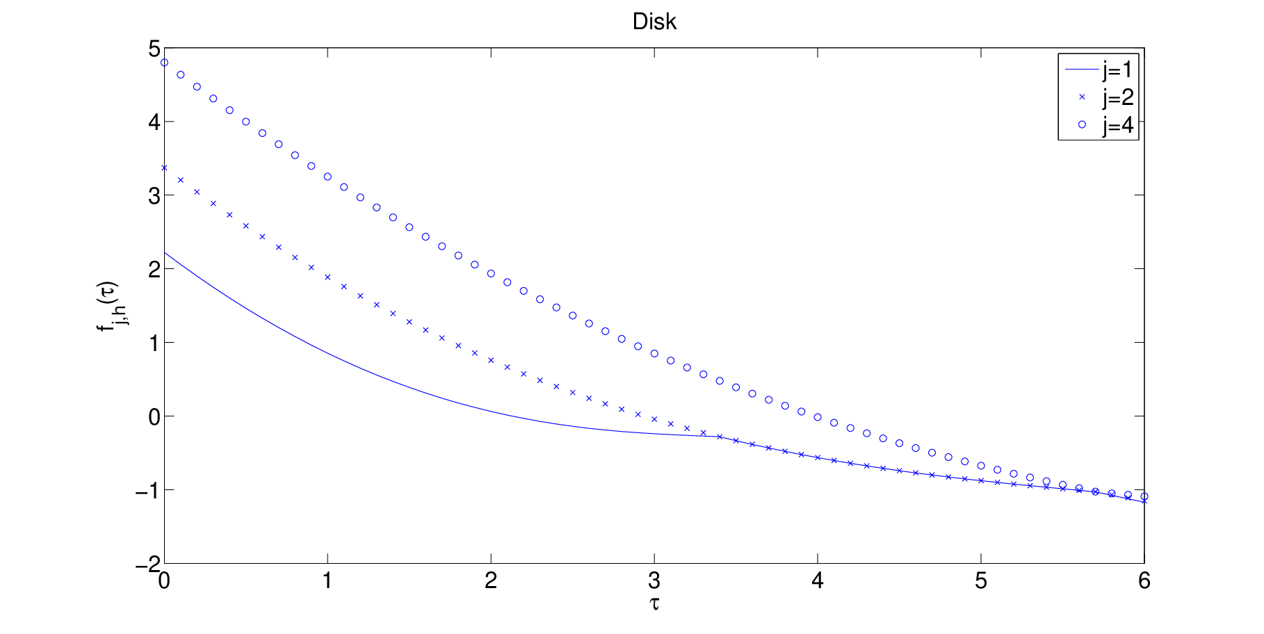
for the three domains, respectively. In Figure 1, we plot fh​(τ)=γh​(τ)−τf_{h}(\tau)=\gamma_{h}(\tau)-\tau for several eigenvalues. The plots show that fhf_{h} is decreasing right to the origin. In fact, it can be seen that fh​(τ)f_{h}(\tau) is decreasing on much larger intervals than those in (6.3) predicted by Theorem 4.2.
Refer to caption
Refer to caption
Refer to caption
Figure 1. Plots of fj,h=γj,h​(τ)−τf_{j,h}=\gamma_{j,h}(\tau)-\tau v.s. τ\tau. Top Left: the disk for j=1,2,4j=1,2,4. Top Right: the unit square for j=1,2,5j=1,2,5. Bottom: the L-shaped domain for j=1,2,3j=1,2,3.

6.3. Real transmission eigenvalues

Next we present the results of the smallest transmission eigenvalues. Table 2 gives the computed eigenvalues and the convergence orders of the first transmission eigenvalue of three domains using the secant method. It can be seen that the convergence rate for the unite square is approximately 22 indicating that the associated eigenfunction u∈H3​(D)u\in H^{3}(D). The convergence rate for the L-shaped domain is much lower, which is likely caused by the low regularity of the eigenfunction. Similar results can be observed for the biharmonic eigenvalue problem (see Chap. 4 of [27] or [7]).

hh Unit square order L-shaped order Circle order
0.1 1.94289620 4.956235 2.151129
0.05 1.94288512 4.911192 2.128551
0.025 1.94287991 1.367706 4.887524 1.166121 2.117252 1.180424
0.0125 1.94287811 1.961417 4.874986 1.529921 2.110723 1.449210
Table 2. Convergence orders of the first real transmission eigenvalue using the secant method.
Remark 6.1.

When the domain is a disk, one can obtain transmission eigenvalues associated with radially-symmetric eigenfunctions using separation of variables. The detail of derivation of such eigenvalues is given in Appendix A.

In Table 3, we show the six smallest transmission eigenvalues computed by the secant method for the three domains with mesh size h≈0.025h\approx 0.025. The method converges in a few steps.

τj\tau_{j} Unit square NOI L-shaped NOI Circle NOI
τ1\tau_{1} 1.942885 7 4.887524 6 2.117252 7
τ2\tau_{2} 2.618883 7 5.314739 5 2.921413 9
τ3\tau_{3} 2.618883 8 6.301718 6 2.921413 12
τ4\tau_{4} 3.247320 6 6.664844 6 3.958629 8
τ5\tau_{5} 3.748613 5 7.418109 7 3.958629 8
τ6\tau_{6} 4.418714 5 8.021953 10 5.175589 6
Table 3. Six smallest transmission eigenvalues computed by the secant method. ”NOI” denotes the number of iterations.

In Table 4, we give the six smallest transmission eigenvalues computed by the secant method for the three domains using a different set of parameters μ=1/5,λ=1/5,ρ0=1/20,ρ1=3\mu=1/5,\lambda=1/5,\rho_{0}=1/20,\rho_{1}=3. The iteration converges in a few steps as well.

τj\tau_{j} Unit square NOI L-shaped NOI Circle NOI
τ1\tau_{1} 6.451568 4 10.882301 4 7.130154 4
τ2\tau_{2} 7.649225 5 13.680402 4 9.062169 5
τ3\tau_{3} 7.649225 5 16.694660 4 9.063492 8
τ4\tau_{4} 11.201158 8 18.281319 5 12.781042 6
τ5\tau_{5} 11.404597 4 19.550610 4 12.782461 8
τ6\tau_{6} 12.099399 6 21.397458 4 14.216742 4
Table 4. Six smallest transmission eigenvalues with μ=1/5,λ=1/5,ρ0=1/20,ρ1=3\mu=1/5,\lambda=1/5,\rho_{0}=1/20,\rho_{1}=3, ”NOI” denotes the number of iterations.

6.4. The special case of disk

From Appendix A, a radially-symmetric transmission eigenvalue of the disk is the first root of Z0Z_{0} defined in (7.3). Using some root finding technique, we find that ω=3.554954\omega=3.554954, i.e., τ=12.637700\tau=12.637700. However, it is not the smallest transmission eigenvalue of the disk. The secant method computes an approximate transmission eigenvalue τ=12.662693\tau=12.662693 with h=0.05h=0.05 and τ=12.624538\tau=12.624538 with h=0.025h=0.025. The mixed method also computes a transmission eigenvalue τ=12.713678\tau=12.713678 with h=0.025h=0.025. Figure 2 plots the eigenfunction 𝒖{\boldsymbol{u}} associated with this eigenvalue, which appear to be radially-symmetric.

Refer to caption
Refer to caption
Refer to caption
Figure 2. A radially-symmetric eigenfunction. Left: u1u_{1}. Middle: u2u_{2}. Right: |𝒖=(u1,u2)||{\boldsymbol{u}}=(u_{1},u_{2})|.

Note that not all eigenfunctions are radially-symmetric. Figure 3 is the eigenfunction associated with the second eigenvalue. Clearly, it is not a radially-symmetric function.

Refer to caption
Refer to caption
Refer to caption
Figure 3. Second eigenfunction. Left: u1u_{1}. Middle: u2u_{2}. Right: |𝒖=(u1,u2)||{\boldsymbol{u}}=(u_{1},u_{2})|.

6.5. Results by the mixed method

For comparison and verification, we also computes the transmission eigenvalues using the mixed method. Table 5 shows the first transmission eigenvalue and convergence rates.

hh Unit square order L-shaped order Circle order
0.1 2.393618 7.117873 2.734748
0.05 2.040967 5.466449 2.221626
0.025 1.967283 2.273017 5.028595 1.983289 2.136957 2.527205
0.0125 1.948971 2.328781 4.907390 2.205551 2.113930 2.225566
Table 5. The first real transmission eigenvalue of the mixed method.

Note that ETE is non-self-adjoint and the secant method only computes real transmission eigenvalues. The mixed method can compute complex eigenvalues. Table 6 gives the convergence orders of the first complex transmission eigenvalue.

hh Unit square order L-shaped order Circle order
0.1 3.335717 - 3.171243i 3.631454 - 3.333002i 4.153116 - 0.863572i
0.05 3.494072 - 1.117876i 3.616318 - 3.116377i 3.963564 - 1.126331i
0.025 3.422905 - 1.097453i 4.450560 3.613011 - 3.061526i 2.049651 3.897421 - 1.131189i 2.137062
0.0125 3.402856 - 1.090597i 2.167773 3.611227 - 3.047409i 2.280984 3.876819 - 1.126730i 2.040988
Table 6. The first complex transmission eigenvalue of the mixed method.

7. Conclusions and Future Work

In this paper, we propose an iterative method to compute a few smallest transmission eigenvalues for elastic waves. The major advantage of this method is the accuracy and effectiveness since we only need to compute a few eigenvalues of Hermitian eigenvalue problems instead of computing the full eigensystem of a non-Hermitian eigenvalue problem. This fits the practical need in the sense that in general only the smallest transmission eigenvalues are needed for the estimation of the elastic properties of the material. We prove the convergence of the proposed method. The effectiveness of the method is verified by some numerical examples. We have also given a mixed method without proof. In future, we will consider the complex eigenvalues of the elastic waves. The analytic property of the function f⁡(τ)=γ⁡(τ)−τf(\tau)=\gamma(\tau)-\tau is also an interesting topic.

Appendix A: Radially Symmetric Case on Disks

We derive the equation satisfied by a transmission eigenvalue whose associated eigenfunction is radially symmetric on a disk. Let D⊂ℝ2D\subset\mathbb{R}^{2} be a disk with radius RR. Let 𝒖=(w,v)⊤{\boldsymbol{u}}=(w,v)^{\top}. Writing the elasticity wave equation (2.1) component wise, we have that

(7.1) (2​μ+λ)​∂2w∂x12+(λ+μ)​∂2v∂x2​∂x1+μ​∂2w∂2x2+ω2​ρ​w=0,\displaystyle(2\mu+\lambda)\frac{\partial^{2}w}{\partial x_{1}^{2}}+(\lambda+\mu)\frac{\partial^{2}v}{\partial x_{2}\partial x_{1}}+\mu\frac{\partial^{2}w}{\partial^{2}x_{2}}+\omega^{2}\rho w=0,
(7.2) (μ+λ)​∂2w∂x2​∂x1+μ​∂2v∂x12+(2​μ+λ)​∂2v∂x22+ω2​ρ​v=0.\displaystyle(\mu+\lambda)\frac{\partial^{2}w}{\partial x_{2}\partial x_{1}}+\mu\frac{\partial^{2}v}{\partial x_{1}^{2}}+(2\mu+\lambda)\frac{\partial^{2}v}{\partial x_{2}^{2}}+\omega^{2}\rho v=0.

If we consider the solution in the form of radially-symmetric vector field 𝒖⁡(𝒙)=u⁡(r)​𝒆r{\boldsymbol{u}}({\boldsymbol{x}})=u(r){\boldsymbol{e}}_{r}, where r=|𝒙|r=|{\boldsymbol{x}}| and 𝒆r=𝒙/r{\boldsymbol{e}}_{r}={\boldsymbol{x}}/{r}, w=u⁡(r)​cos⁡θ,v=u⁡(r)​sin⁡θw=u(r)\cos\theta,v=u(r)\sin\theta, (7.1) can be written as

(μ+λ)​(∂2w∂x12+∂2v∂x2​∂x1)+μ⁡(∂2w∂2x2+∂2w∂x12)+ω2​ρ​w=0.(\mu+\lambda)\left(\frac{\partial^{2}w}{\partial x_{1}^{2}}+\frac{\partial^{2}v}{\partial x_{2}\partial x_{1}}\right)+\mu\left(\frac{\partial^{2}w}{\partial^{2}x_{2}}+\frac{\partial^{2}w}{\partial x_{1}^{2}}\right)+\omega^{2}\rho w=0.

Using polar coordinate, (7.1) becomes

(λ+μ)​(ur​r+1r​ur−1r2​u)+μ⁡(ur​r+1r​ur−1r2​u)+ω2​ρ​u=0,(\lambda+\mu)\left(u_{rr}+\frac{1}{r}u_{r}-\frac{1}{r^{2}}u\right)+\mu\left(u_{rr}+\frac{1}{r}u_{r}-\frac{1}{r^{2}}u\right)+\omega^{2}\rho u=0,

i.e.,

(λ+2​μ)​(ur​r+1r​ur−1r2​u)+ω2​ρ​u=0.(\lambda+2\mu)\left(u_{rr}+\frac{1}{r}u_{r}-\frac{1}{r^{2}}u\right)+\omega^{2}\rho u=0.

Similarly, (7.2) is simply

(μ+λ)​(ur​r+1r​ur−1r2​u)+μ⁡(ur​r+1r​ur−1r2​u)+ω2​ρ​u=0,(\mu+\lambda)\left(u_{rr}+\frac{1}{r}u_{r}-\frac{1}{r^{2}}u\right)+\mu\left(u_{rr}+\frac{1}{r}u_{r}-\frac{1}{r^{2}}u\right)+\omega^{2}\rho u=0,

i.e.,

(2​μ+λ)​(ur​r+1r​ur−1r2​u)+ω2​ρ​u=0.(2\mu+\lambda)\left(u_{rr}+\frac{1}{r}u_{r}-\frac{1}{r^{2}}u\right)+\omega^{2}\rho u=0.

The above equation can be written as

r2​d2​ud​r2+r​d​ud​r+(r2​ω2​ρ2​μ+λ−1)​u=0.r^{2}\frac{{\rm d}^{2}u}{{\rm d}r^{2}}+r\frac{{\rm d}u}{{\rm d}r}+\left(r^{2}\frac{\omega^{2}\rho}{2\mu+\lambda}-1\right)u=0.

The solution of the above equation is given by the Bessel function of order one J1​(a​r)J_{1}(ar), where

a=ω​ρ2​μ+λ.a=\omega\sqrt{\frac{\rho}{2\mu+\lambda}}.

Then we obtain that 𝒖=(w,v)⊤:=(J1​(a​r)​cos⁡θ,J1​(a​r)​sin⁡θ)⊤{\boldsymbol{u}}=(w,v)^{\top}:=(J_{1}(ar)\cos\theta,J_{1}(ar)\sin\theta)^{\top}.

Next we look at the boundary condition involving σ⁡(𝒖)​𝝂\sigma({\boldsymbol{u}}){\boldsymbol{\nu}}. For the transmission eigenvalue problem, we assume that

𝒖=(J1​(a1​r)​cos⁡θJ1​(a1​r)​sin⁡θ),𝒗=C​(J1​(a2​r)​cos⁡θJ1​(a2​r)​sin⁡θ),{\boldsymbol{u}}=\begin{pmatrix}J_{1}(a_{1}r)\cos\theta\\ J_{1}(a_{1}r)\sin\theta\end{pmatrix},\quad{\boldsymbol{v}}=C\begin{pmatrix}J_{1}(a_{2}r)\cos\theta\\ J_{1}(a_{2}r)\sin\theta\end{pmatrix},

where CC is a constant to be determined from (2.4) and

a1=ω​ρ12​μ+λ,a2=ω​ρ22​μ+λ.a_{1}=\omega\sqrt{\frac{\rho_{1}}{2\mu+\lambda}},\quad a_{2}=\omega\sqrt{\frac{\rho_{2}}{2\mu+\lambda}}.

Note that 𝝂=(ν1,ν2)⊤=(cos⁡θ,sin⁡θ)T{\boldsymbol{\nu}}=(\nu_{1},\nu_{2})^{\top}=(\cos\theta,\sin\theta)^{T}. It follows from (2.2) that the first component of σ⁡(𝒖)​𝝂\sigma({\boldsymbol{u}}){\boldsymbol{\nu}} is

λ⁡[∂∂r​J​(a​r)+1r​J​(a​r)]​cos⁡θ+2​μ​∂∂r​J​(a​r)​cos⁡θ.\displaystyle\lambda\left[\frac{\partial}{\partial r}J(ar)+\frac{1}{r}J(ar)\right]\cos\theta+2\mu\frac{\partial}{\partial r}J(ar)\cos\theta.

The second component of σ⁡(𝒖)​𝝂\sigma({\boldsymbol{u}}){\boldsymbol{\nu}} is

2​μ​∂∂r​J​(a​r)​sin⁡θ+λ⁡[∂∂r​J​(a​r)+1r​J​(a​r)]​sin⁡θ.\displaystyle 2\mu\frac{\partial}{\partial r}J(ar)\sin\theta+\lambda\left[\frac{\partial}{\partial r}J(ar)+\frac{1}{r}J(ar)\right]\sin\theta.

Using the boundary conditions (2.4), we obtain

C=J1​(a1​R)J1​(a2​R),C=\frac{J_{1}(a_{1}R)}{J_{1}(a_{2}R)},

and

(2​μ​∂∂r​J​(a1​r)+λ⁡[∂∂r​J​(a1​r)+1r​J​(a1​r)])|r=R=C⁡(2​μ​∂∂r​J​(a2​r)+λ⁡[∂∂r​J​(a2​r)+1r​J​(a2​r)])|r=R.\left(2\mu\frac{\partial}{\partial r}J(a_{1}r)+\lambda\left[\frac{\partial}{\partial r}J(a_{1}r)+\frac{1}{r}J(a_{1}r)\right]\right)\Big|_{r=R}=C\left(2\mu\frac{\partial}{\partial r}J(a_{2}r)+\lambda\left[\frac{\partial}{\partial r}J(a_{2}r)+\frac{1}{r}J(a_{2}r)\right]\right)\Big|_{r=R}.

Hence ω\omega is a transmission eigenvalue if it satisfies

(7.3) Z0​(ω):=|J1​(a1​R)J1​(a2​R)a1​J1′​(a1​R)a2​J1′​(a2​R)|=0.Z_{0}(\omega):=\left|\begin{array}[]{cc}J_{1}\left(a_{1}R\right)&J_{1}\left(a_{2}R\right)\\ a_{1}J_{1}^{\prime}(a_{1}R)&a_{2}J_{1}^{\prime}(a_{2}R)\end{array}\right|=0.

Figure 4 is the contour plot of |Z0​(ω)||Z_{0}(\omega)| on the complex plane.

Refer to caption
Figure 4. The contour plot of |Z0​(ω)||Z_{0}(\omega)| with μ=1/16,λ=1/4,ρ0=1,ρ1=4\mu=1/16,\lambda=1/4,\rho_{0}=1,\rho_{1}=4. The centers of the circular curves indicate the locations of transmission eigenvalues.

Appendix B: Imposing Boundary Conditions

The boundary condition for VV needs careful treatment for the Argyris element. On one boundary of a triangle γe⊂𝒯\gamma_{e}\subset\mathcal{T} with unit outward normal (nx,ny)(n_{x},n_{y}) and unit tangential vector (τx,τy)(\tau_{x},\tau_{y}), we consider the case nx​ny≠0n_{x}n_{y}\neq 0. Otherwise it is easy to figure out. It is clear that

(7.4) τx​nx+τy​ny=0,τx2+τy2=1,nx2+ny2=1.\tau_{x}n_{x}+\tau_{y}n_{y}=0,\quad\tau_{x}^{2}+\tau_{y}^{2}=1,\quad n_{x}^{2}+n_{y}^{2}=1.

On the boundary γe\gamma_{e}, 𝒖=(u1,u2)⊤=𝟎\boldsymbol{u}=(u_{1},u_{2})^{\top}=\boldsymbol{0}, so the tangent derivatives are also 𝟎\boldsymbol{0}, i.e.,

∂u1∂x​τx+∂u1∂y​τy=0,∂u2∂x​τx+∂u2∂y​τy=0.\frac{\partial u_{1}}{\partial x}\tau_{x}+\frac{\partial u_{1}}{\partial y}\tau_{y}=0,\quad\frac{\partial u_{2}}{\partial x}\tau_{x}+\frac{\partial u_{2}}{\partial y}\tau_{y}=0.

The boundary condition σ⁡(𝒖)​𝝂=𝟎\sigma(\boldsymbol{u}){\boldsymbol{\nu}}=\boldsymbol{0} means

((λ+2​μ)​∂xu1+λ​∂yu2)​nx+μ⁡(∂yu1+∂xu2)​ny=0,\displaystyle((\lambda+2\mu)\partial_{x}u_{1}+\lambda\partial_{y}u_{2})n_{x}+\mu(\partial_{y}u_{1}+\partial_{x}u_{2})n_{y}=0,
μ⁡(∂xu2+∂yu1)​nx+(λ​∂xu1+(λ+2​μ)​∂yu2)​ny=0.\displaystyle\mu(\partial_{x}u_{2}+\partial_{y}u_{1})n_{x}+(\lambda\partial_{x}u_{1}+(\lambda+2\mu)\partial_{y}u_{2})n_{y}=0.

Substituting

∂u1∂y=−τxτy​∂u1∂x,∂u2∂y=−τxτy​∂u2∂x,\frac{\partial u_{1}}{\partial y}=-\frac{\tau_{x}}{\tau_{y}}\frac{\partial u_{1}}{\partial x},\quad\frac{\partial u_{2}}{\partial y}=-\frac{\tau_{x}}{\tau_{y}}\frac{\partial u_{2}}{\partial x},

into above equations, we have

(λ+2​μ)​∂xu1​nx−τxτy​λ​∂xu2​nx−τxτy​μ​∂xu1​ny+μ​∂xu2​ny=0,\displaystyle(\lambda+2\mu)\partial_{x}u_{1}n_{x}-\frac{\tau_{x}}{\tau_{y}}\lambda\partial_{x}u_{2}n_{x}-\frac{\tau_{x}}{\tau_{y}}\mu\partial_{x}u_{1}n_{y}+\mu\partial_{x}u_{2}n_{y}=0,
μ​∂xu2​nx−τxτy​μ​∂xu1​nx+λ​∂xu1​ny−τxτy​(λ+2​μ)​∂xu2​ny=0,\displaystyle\mu\partial_{x}u_{2}n_{x}-\frac{\tau_{x}}{\tau_{y}}\mu\partial_{x}u_{1}n_{x}+\lambda\partial_{x}u_{1}n_{y}-\frac{\tau_{x}}{\tau_{y}}(\lambda+2\mu)\partial_{x}u_{2}n_{y}=0,

i.e.,

∂xu1​[nx​(λ+2​μ)−μ​τxτy​ny]+∂xu2​[μ​ny−τxτy​λ​nx]=0,\displaystyle\partial_{x}u_{1}[n_{x}(\lambda+2\mu)-\mu\frac{\tau_{x}}{\tau_{y}}n_{y}]+\partial_{x}u_{2}[\mu n_{y}-\frac{\tau_{x}}{\tau_{y}}\lambda n_{x}]=0,
∂xu1​[λ​ny−τxτy​μ​nx]+∂xu2​[μ​nx−(λ+2​μ)​ny​τxτy]=0,\displaystyle\partial_{x}u_{1}[\lambda n_{y}-\frac{\tau_{x}}{\tau_{y}}\mu n_{x}]+\partial_{x}u_{2}[\mu n_{x}-(\lambda+2\mu)n_{y}\frac{\tau_{x}}{\tau_{y}}]=0,

which yields

∂xu1​[τy​nx​(λ+2​μ)−μ​τx​ny]−∂xu2​(λ+μ)​nx​τx=0,\displaystyle\partial_{x}u_{1}[\tau_{y}n_{x}(\lambda+2\mu)-\mu\tau_{x}n_{y}]-\partial_{x}u_{2}(\lambda+\mu)n_{x}\tau_{x}=0,
−∂xu1(λ+μ)nxτx+∂xu2[μnxτy−(λ+2μ)nyτx]=0.\displaystyle-\partial_{x}u_{1}(\lambda+\mu)n_{x}\tau_{x}+\partial_{x}u_{2}[\mu n_{x}\tau_{y}-(\lambda+2\mu)n_{y}\tau_{x}]=0.

Here we have used the fact that τx​nx+τy​ny=0\tau_{x}n_{x}+\tau_{y}n_{y}=0. Using (7.4), the determination of the above equations is

μ⁡(λ+2​μ)​nx2​(1−τx2)+μ⁡(λ+2​μ)​τx2​(1−nx2)+(λ+2​μ)2​nx2​τx2+μ2​nx2​τx2−(λ+μ)2​nx2​τx2\displaystyle\mu(\lambda+2\mu)n_{x}^{2}(1-\tau_{x}^{2})+\mu(\lambda+2\mu)\tau_{x}^{2}(1-n_{x}^{2})+(\lambda+2\mu)^{2}n_{x}^{2}\tau_{x}^{2}+\mu^{2}n_{x}^{2}\tau_{x}^{2}-(\lambda+\mu)^{2}n_{x}^{2}\tau_{x}^{2}
=\displaystyle= μ⁡(λ+2​μ)​(nx2+τx2)+nx2​τx2​((λ+2​μ)2+μ2−(λ+μ)2−2​μ​(λ+2​μ))\displaystyle\mu(\lambda+2\mu)(n_{x}^{2}+\tau_{x}^{2})+n_{x}^{2}\tau_{x}^{2}((\lambda+2\mu)^{2}+\mu^{2}-(\lambda+\mu)^{2}-2\mu(\lambda+2\mu))
=\displaystyle= μ⁡(λ+2​μ)​(nx2+τx2)>0.\displaystyle\mu(\lambda+2\mu)(n_{x}^{2}+\tau_{x}^{2})>0.

Consequently,

∂xu1=∂yu1=∂xu2=∂yu2=0.\partial_{x}u_{1}=\partial_{y}u_{1}=\partial_{x}u_{2}=\partial_{y}u_{2}=0.

The tangential derivatives of all the first-order derivatives are 0. Taking u1u_{1} for example, we have

∂2u1∂x2​τx+∂2u1∂x​∂y​τy=0,\displaystyle\frac{\partial^{2}u_{1}}{\partial x^{2}}\tau_{x}+\frac{\partial^{2}u_{1}}{\partial x\partial y}\tau_{y}=0,
∂2u1∂x​∂y​τx+∂2u1∂y2​τy=0,\displaystyle\frac{\partial^{2}u_{1}}{\partial x\partial y}\tau_{x}+\frac{\partial^{2}u_{1}}{\partial y^{2}}\tau_{y}=0,

which implies

(7.5) ∂2u1∂x2=−τy2τx2​∂2u1∂y2,∂2u1∂x​∂y=−τyτx​∂2u1∂y2.\frac{\partial^{2}u_{1}}{\partial x^{2}}=-\frac{\tau^{2}_{y}}{\tau^{2}_{x}}\frac{\partial^{2}u_{1}}{\partial y^{2}},\quad\frac{\partial^{2}u_{1}}{\partial x\partial y}=-\frac{\tau_{y}}{\tau_{x}}\frac{\partial^{2}u_{1}}{\partial y^{2}}.

If a point belonging to two edges γe​1\gamma_{e1} and γe​2\gamma_{e2} satisfies (7.5) with different tangential derivatives, we have

∂2u1∂x2=∂2u1∂y2=∂2u1∂x​∂y=0.\frac{\partial^{2}u_{1}}{\partial x^{2}}=\frac{\partial^{2}u_{1}}{\partial y^{2}}=\frac{\partial^{2}u_{1}}{\partial x\partial y}=0.

References

  • [1] J. An and J. Shen, A Fourier-spectral-element method for transmission eigenvalue problems, J. Sci. Comput. 57 (2013), 670–688.
  • [2] I. Babuška and J. Osborn, Eigenvalue problems, in Handbook of Numerical Analysis II, P. Ciarlet and J. Lions, eds., North-Holland, Amsterdam, 1991, 641–787.
  • [3] C. Bellis, F. Cakoni, and B. Guzina, Nature of the transmission eigenvalue spectrum for elastic bodies, IMA J. Appl. Math. 78 (2013), 895–923.
  • [4] C. Bellis and B. Guzina, On the existence and uniqueness of a solution to the interior transmission problem for piecewise-homogeneous solids, J. Elasticity 101 (2010), 29–57.
  • [5] S. Brenner and L. Scott, The mathematical theory of finite elements methods, 2nd Edition, Texts in Applied Mathematics, Springer, 2002.
  • [6] H. Blum and R. Rannacher, On the boundary value problem of the biharmonic operator on domains with angular corners, Math. Methods Appl. Sci. 2 (1980), 556–581.
  • [7] S. Brenner, P. Monk, and J. Sun, C0C^{0} interior penalty Galerkin method for biharmonic eigenvalue problems, Spectral and High Order Methods for Partial Differential Equations, Lect. Notes Comput. Sci. Eng. 106 (2015), 3–15.
  • [8] F. Cakoni, D. Colton, P. Monk and J. Sun, The inverse electromagnetic scattering problem for anisotropic media, Inver. Probl. 26 (2010), 074004.
  • [9] F. Cakoni, P. Monk, and J. Sun, Error analysis of the finite element approximation of transmission eigenvalues, Comput. Methods Appl. Math. 14 (2014), 419–427.
  • [10] A. Charalambopoulos, On the interior transmission problem in nondissipative, inhomogeneous, anisotropic elasticity, J. Elasticity 67 (2002), 149–170.
  • [11] A. Charalambopoulos and K. Anagnostopoulos, On the spectrum of the interior transmission problem in isotropic elasticity, J. Elasticity 90 (2008), 295–313.
  • [12] D. Colton, P. Monk, and J. Sun, Analytical and computational methods for transmission eigenvalues, Inver. Probl. 26 (2010), 045011.
  • [13] P. Ciarlet, The finite element method for elliptic problems, Classics in Applied Mathematics, 40, SIAM, Philadelphia, 2002.
  • [14] P. Grisvard, Elliptic problems in nonsmooth domains, Pitman, Boston, 1985.
  • [15] J. Marsden and T. Hughes, Mathematical of foundations of elasticity, Dover, 1994.
  • [16] T. Huang, W. Huang, and W. Lin, A robust numerical algorithm for computing Maxwell’s transmission eigenvalue problems, SIAM J. Sci. Comput. 37 (2015), A2403–A2423.
  • [17] R. Huang, A. Struthers, J. Sun, and R. Zhang, Recursive integral method for transmission eigenvalues, J. Comput. Phys. 327 (2016), 830–840.
  • [18] R. Huang, J. Sun and C. Yang, Recursive integral method with Cayley transformation, arXiv:1705.01646, 2017.
  • [19] A. Kleefeld, A numerical method to compute interior transmission eigenvalues. Inver. Probl. 29 (2013), 104012.
  • [20] T. Li, W. Huang, W. Lin, and J. Liu, On spectral analysis and a novel algorithm for transmission eigenvalue problems, J. Sci. Comput. 64 (2015), 83–108.
  • [21] X. Ji, J. Sun, and T. Turner, A mixed finite element method for Helmholtz transmission eigenvalues, ACM Trans. Math. Software 8 (2012), Algorithm 922.
  • [22] X. Ji, J. Sun, and H. Xie, A multigrid method for Helmholtz transmission eigenvalue problem, J. Sci. Comput. 60 (2014), 276–294.
  • [23] P. Monk and J. Sun, Finite element methods of Maxwell transmission eigenvalues, SIAM J. Sci. Comput. 34 (2012), B247–B264.
  • [24] J. Sun, Iterative methods for transmission eigenvalues, SIAM J. Numer. Anal. 49 (2011), 1860–1874.
  • [25] J. Sun, Estimation of transmission eigenvalues and the index of refraction from Cauchy data, Inver. Probl. 27 (2011), 015009.
  • [26] J. Sun and L. Xu, Computation of the Maxwell’s transmission eigenvalues and its application in inverse medium problems, Inver. Probl. 29 (2013), 104013.
  • [27] J. Sun and A. Zhou, Finite element methods for eigenvalue problems, CRC Press, Taylor & Francis Group, Boca Raton, London, New York, 2016.
  • [28] Y. Yang, H. Bi, H. Li, and J. Han, Mixed methods for the Helmholtz transmission eigenvalues, SIAM J. Sci. Comput. 38 (2016), A1383–A1403.