Battery Energy Storage Scheduling for Optimal Load Variance MinimizationThanks: Research sponsored by the Laboratory Directed Research and Development Program of Oak Ridge National Laboratory (ORNL), managed by UT-Battelle, LLC for the U.S. Department of Energy under Contract No. DE-AC05-00OR22725. The submitted manuscript has been authored by a contractor of the U.S. Government under Contract DE-AC05-00OR22725. Accordingly, the U.S. Government retains a nonexclusive, royalty-free license to publish or reproduce the published form of this contribution, or allow others to do so, for U.S. Government purposes.

Let $P_{Bc}(t)$ and $P_{Bd}(t)$ denote total BES charging and discharging powers, respectively. Let $P_{L}(t)$ denote the forecasted total load profile, which is assumed to be known in this paper. Loss is neglected for now. Then, the power at PCC $P_{g}(t)$ can be expressed as follows

$\displaystyle P_{g}(t)=P_{Bc}(t)-P_{Bd}(t)+P_{L}(t)$

(1)

where $P_{Bc}(t)>0$ and $P_{Bd}(t)>0$. The objective is to minimize the demand peak-valley gap. To explore the optimality, the ideal case is set as the target curve, where there is no peak-valley gap illustrated as the red line in Fig. 1. Then, the objective can be expressed as the infinity norm minimization as follows

$\displaystyle\underset{P_{Bc}(t),P_{Bd}(t)}{\min}\lVert P_{Bc}(t)-P_{Bd}(t)+P_{L}(t)-\theta\rVert_{\infty}$

(2)

In robust control, instead of minimizing $||T_{zw}||_{\infty}$, it is usually desired to minimize the upper bound $\gamma$, where $||T_{zw}||_{\infty}<\gamma$ and $\gamma>0$ [18]. Similar idea is applied into the objective reformulation as the objective in (2) is equivalent to

$\displaystyle\underset{P_{Bc}(t),P_{Bd}(t)}{\min}\quad K$

(3)

such that

$\displaystyle 0\leq\mid P_{Bc}(t)-P_{Bd}(t)+P_{L}(t)-\theta\mid\leq K$

(4)

There are two ways to deal with the target curve $\theta$. One is to treat $\theta$ as a given constant. The second approach is to regard $\theta$ as a decision variable. Since here the objective is to minimize the variance of the power at PCC, so $\theta$ needs to be limited between the valley and peak of forecasted load. Then the alternative problem can be formulated as

$\displaystyle\underset{P_{Bc}(t),P_{Bd}(t),\theta}{\min}\quad\alpha K+\beta\theta$

(5)

such that

		$\displaystyle 0\leq\mid P_{Bc}(t)-P_{Bd}(t)+P_{L}(t)-\theta\mid\leq K$		(6)
		$\displaystyle\min{P_{L}(t)}\leq\theta\leq\max{P_{L}(t)},\alpha>0,\beta>0$

Let $\mathcal{E}$ denote the set of buses that have BES and load connected. The battery model can be expressed as follows [19]

$\displaystyle E_{b,i}(t)=E_{b,i}(t-1)+\eta TP_{bc,i}(t)-\frac{1}{\eta}TP_{bd,i}(t)\quad\forall i\in\mathcal{E}$

(8)

where $P_{bc,i}(t)$ and $P_{bd,i}(t)$ are charging and discharging power of BES at bus $i$ in kW. $E_{b,i}(t)$ is the available capacity of BES at bus $i$ (kW$\cdot$h). $\eta$ represents the BES charging/discharging efficiency. $T$ is the time interval. The BES capacity limit can be expressed by the following constraints

$\displaystyle\text{SOC}_{\min}B_{\text{cap}}\leq E_{b,i}(t)\leq\text{SOC}_{\max}B_{\text{cap}}\quad\forall i\in\mathcal{E}$

(9)

where $B_{\text{cap}}$ is the rated capacity in kW$\cdot$h. $\text{SOC}_{\min}$ and $\text{SOC}_{\max}$ are the state-of-charge limits in percentage. In general, simultaneous charging and discharging is unrealistic. Binary variable can be introduced to force only one action to be activated during each scheduling interval $T$ [20] as follows

		$\displaystyle P_{Bc}(t)=\sum_{i\in\mathcal{E}}P_{bc,i}(t),P_{Bd}(t)=\sum_{i\in\mathcal{E}}P_{bd,i}(t)$		(10)
		$\displaystyle 0\leq P_{bc,i}(t)\leq P_{bc,\max}m_{bc,i}(t)\quad\forall i\in\mathcal{E}$
		$\displaystyle 0\leq P_{bd,i}(t)\leq P_{bd,\max}m_{bd,i}(t)\quad\forall i\in\mathcal{E}$
		$\displaystyle m_{bc,i}(t)+m_{bd,i}(t)\leq 1\quad\forall i\in\mathcal{E}$

where $P_{bc,\max}$ and $P_{bd,\max}$ are the BES charging and discharging power limits. $m_{bc,i}(t)$ and $m_{bd,i}(t)$ are binary variables representing the operating modes of charging and discharging. 1 means the corresponding mode is activated while 0 stands for deactivation. The last constraint in Eq. (10) ensures no simultaneous charging and discharging situation.

The distribution network power flow (DistFlow) is borrowed from [15] and more generally from [16] including lateral branches, which has been employed in [21] for microgrid scheduling. Consider a radial distribution network shown in Fig. 2. Let $\mathcal{N}$ denote the set of buses that only have load connected. The following equations can be used to describe the complex power flows at each node $i$ at time $t$

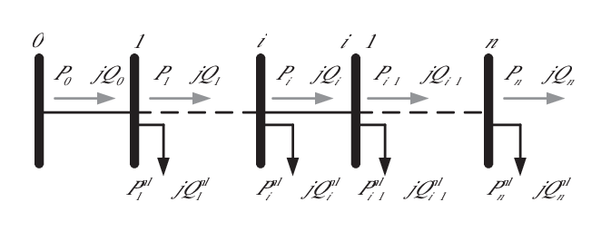
		$\displaystyle P_{i+1}(t)=P_{i}(t)-r_{i}\dfrac{P_{i}^{2}(t)+Q_{i}^{2}(t)}{V_{i}^{2}(t)}-P_{\text{nl},i+1}(t)$		(11)
		$\displaystyle Q_{i+1}(t)=Q_{i}(t)-x_{i}\dfrac{P_{i}^{2}(t)+Q_{i}^{2}(t)}{V_{i}^{2}(t)}-Q_{\text{nl},i+1}(t)$
		$\displaystyle V_{i+1}^{2}(t)=V_{i}^{2}(t)-2[r_{i}P_{i}(t)+x_{i}Q_{i}(t)]+(r_{i}^{2}+x_{i}^{2})\dfrac{P_{i}^{2}(t)+Q_{i}^{2}(t)}{V_{i}^{2}(t)}$

where nl stands for net load. $x_{i}$ is inductance from branch $i$ to $i+1$. $P_{i}$ and $Q_{i}$ are the load flow from branch $i$ to $i+1$. The first approximation is made by dropping the quadratic terms as the branch losses are much smaller than the branch power [16]. Then, the simplified DistFlow is shown as

		$\displaystyle P_{i+1}(t)=P_{i}(t)-P_{\text{nl},i+1}(t)$		(12)
		$\displaystyle Q_{i+1}(t)=Q_{i}(t)-Q_{\text{nl},i+1}(t)$
		$\displaystyle V_{i+1}^{2}(t)=V_{i}^{2}(t)-2[r_{i}P_{i}(t)+x_{i}Q_{i}(t)]$

The second approximation is made by the following assumption in [17]

$\displaystyle\left[V_{i}(t)-V_{0}(t)\right]^{2}\approx 0,$

(13)

which leads to

$\displaystyle V_{i}^{2}(t)\approx V_{0}^{2}(t)+2V_{0}(t)[V_{i}(t)-V_{0}(t)]$

(14)

The rationality of the second approximation lies in the fact that the per unit voltage variation along the line remain within the bounds for proper operation of a distribution system as

$\displaystyle 1-\epsilon\leq V_{i}(t)\leq 1+\epsilon$

(15)

where $\epsilon>0$ is generally very small [17]. After the two approximations, the DistFlow equations become

		$\displaystyle P_{i+1}(t)=P_{i}(t)-P_{i+1}^{\text{nl}}(t),Q_{i+1}(t)=Q_{i}(t)-Q_{i+1}^{\text{nl}}(t)$		(16)
		$\displaystyle V_{i+1}(t)=V_{i}(t)-\dfrac{r_{i}P_{i}(t)+x_{i}Q_{i}(t)}{V_{0}(t)},P_{L}(t)=\sum_{i\in\mathcal{E}\cup\mathcal{N}}P_{l,i}(t)$
		$\displaystyle P_{\text{nl},i}(t)=P_{l,i}(t),Q_{\text{nl},i}(t)=Q_{l,i}(t)\quad\forall i\in\mathcal{N}$
		$\displaystyle P_{\text{nl},i}(t)=P_{l,i}(t)+P_{bc,i}(t)-P_{bd,i}(t)\quad\forall i\in\mathcal{E}$
		$\displaystyle Q_{\text{nl},i}(t)=Q_{l,i}(t)+Q_{bc,i}(t)-Q_{bd,i}(t)\quad\forall i\in\mathcal{E}$

The terminal condition is given as $P_{n}(t)=0$ and $Q_{n}(t)=0$ for all $t$. As we can see, by restricting the voltage variation the BES power is confined. Consequently, this turns out to be another constraint for load variance minimization.

The lumped system shown in Fig. 3 is employed to study the property of the formulation. The system consists of one aggregated BES and load, and is assumed to be lossless. Consider the first optimization problem

		$\displaystyle\underset{P_{Bc}(t),P_{Bd}(t)}{\min}\quad K$		(17)
		$\displaystyle\text{s.t. }(\ref{eq_main1_cons}),(\ref{eq_bes_dyn}),(\ref{eq_bes_cap}),(\ref{eq_bes_power})$

The problem in (17) is a mix-integer linear programming (MILP). Let $\theta=1830$. The load flattening results when BES capacity equals to 1200 kW$\cdot$h, 1600 kW$\cdot$h and 2200 kW$\cdot$h are shown in Fig. 4. Based on the scheduling results using (17), when $B_{\text{cap}}\geq 2040\text{ kW}\cdot\text{h}$, the load flattening attains the best performance, where $K=0$.

As expected, the value of objective function varies with the choice of $\theta$. The relationship curve under different BES capacity is studied and illustrated in Fig. 5. As shown, when the BES capacity is less than or equal to the critical capacity limit, there is only one choice of $\theta$ that can reach the best load flattening performance under that particular capacity limit. After the critical limit, larger BES capacity will lead to wider range of $\theta$ that can minimize the load variance to zero shown as the flat bottom in Fig. 5. In these scenarios, it is always desired to use the smallest $\theta$ for cost reduction, which corresponds to the left turning point at the flat bottom. This critical choice of $\theta$ enables the energy balance between peak shaving and valley filling. It should be mentioned that the curves will be altered when the BES unit starts from a different initial condition.

Regarding $\theta$ as another decision variable yields:

		$\displaystyle\underset{P_{Bc}(t),P_{Bd}(t)}{\min}\quad\alpha K+\beta\theta$		(18)
		$\displaystyle\text{s.t. }(\ref{eq_main2_cons}),(\ref{eq_bes_dyn}),(\ref{eq_bes_cap}),(\ref{eq_bes_power})$

The scheduling results are summarized in Tab. I. When $\alpha>\beta$, the values of the objective function are exactly those turning points in Fig. 5. However, once $\alpha<\beta$, $\theta$ is minimized with priority and pushed to its lower limit. Thus, the infinity norms are much larger than those in the first case. The scheduled power at PCC of these two cases with different BES capacity is shown in Fig. (6). When the BES capacity is larger than the critical value, although the values of the objective function are different, the scheduled results are the same. But it is not the case when the BES capacity is not adequate for a perfect flattening.

In this section, the lumped system is expanded into a 18-bus radial feeder to study the voltage constraint. Loss is considered in this case. The same total net active load in previous section is used, and distributed to each bus according to Tab. II. The reactive load is assumed to be fixed and given in Tab. II as well. Based on the study in the last subsection, Formulation 2 is chosen with larger weighting factor on infinity norm $K$ than target $\theta$, which leads to

		$\displaystyle\underset{P_{Bc}(t),P_{Bd}(t)}{\min}\quad\alpha K+\beta\theta$		(19)
		$\displaystyle\text{s.t. }(\ref{eq_main2_cons}),(\ref{eq_bes_dyn}),(\ref{eq_bes_cap}),(\ref{eq_bes_power}),(\ref{eq_volt_cons}),(\ref{eq_simp_flow}),\alpha>\beta$

One BES with adequate size of 2200 kW$\cdot$h is deployed in different nodes and the scheduled power at PCC is shown in Fig. 7. Due to the voltage constraint, when the BES is deployed at the end of the network, the charging power is limited to further limit the voltage drop along the line. When the deployment location is moving forward, the scheduled power is approaching the best performance as expected. The best performance is achieved when the BES is deployed at bus 13 or any bus ahead of bus 13.

References

- [1] What the duck curve tells us about managing a green grid. California ISO. [Online]. Available: https://www.caiso.com/Documents/FlexibleResourcesHelpRenewables_FastFacts.pdf
- [2] B. M. Sanandaji, T. L. Vincent, and K. Poolla, “Ramping rate flexibility of residential hvac loads,” IEEE Trans. Sustain. Energy, vol. 7, no. 2, pp. 865–874, 2016.
- [3] A. Majzoobi and A. Khodaei, “Application of microgrids in supporting distribution grid flexibility,” IEEE Trans. Power Syst., vol. 32, no. 5, pp. 3660–3669, 2017.
- [4] Z. Wang and S. Wang, “Grid power peak shaving and valley filling using vehicle-to-grid systems,” IEEE Trans. Power Del., vol. 28, no. 3, pp. 1822–1829, 2013.
- [5] M. Rowe, T. Yunusov, S. Haben, C. Singleton, W. Holderbaum, and B. Potter, “A peak reduction scheduling algorithm for storage devices on the low voltage network,” IEEE Trans. Smart Grid, vol. 5, no. 4, pp. 2115–2124, 2014.
- [6] K. A. Joshi and N. M. Pindoriya, “Day-ahead dispatch of battery energy storage system for peak load shaving and load leveling in low voltage unbalance distribution networks,” in Proc. IEEE PES Innov. Smart Grid Technol. (ISGT), 2015, pp. 1–5.
- [7] L. Jian, H. Xue, G. Xu, X. Zhu, D. Zhao, and Z. Shao, “Regulated charging of plug-in hybrid electric vehicles for minimizing load variance in household smart microgrid,” IEEE Trans. Ind. Electron., vol. 60, no. 8, pp. 3218–3226, 2013.
- [8] M. J. E. Alam, K. M. Muttaqi, and D. Sutanto, “A controllable local peak-shaving strategy for effective utilization of pev battery capacity for distribution network support,” IEEE Trans. Ind. Appl., vol. 51, no. 3, pp. 2030–2037, 2015.
- [9] M. H. Albadi and E. F. El-Saadany, “A summary of demand response in electricity markets,” Electr. Power Syst. Res., vol. 78, no. 11, pp. 1989–1996, 2008.
- [10] D. Caprino, M. L. Della Vedova, and T. Facchinetti, “Peak shaving through real-time scheduling of household appliances,” Energy and Buildings, vol. 75, pp. 133–148, 2014.
- [11] P. Malysz, S. Sirouspour, and A. Emadi, “An optimal energy storage control strategy for grid-connected microgrids,” IEEE Trans. Smart Grid, vol. 5, no. 4, pp. 1785–1796, 2014.
- [12] K. Worthmann, C. M. Kellett, P. Braun, L. Grüne, and S. R. Weller, “Distributed and decentralized control of residential energy systems incorporating battery storage,” IEEE Trans. Smart Grid, vol. 6, no. 4, pp. 1914–1923, 2015.
- [13] R. Khodabakhsh and S. Sirouspour, “Optimal control of energy storage in a microgrid by minimizing conditional value-at-risk,” IEEE Trans. Sustain. Energy, vol. 7, no. 3, pp. 1264–1273, 2016.
- [14] Y. Levron and D. Shmilovitz, “Power systems’ optimal peak-shaving applying secondary storage,” Electr. Power Syst. Res., vol. 89, pp. 80–84, 2012.
- [15] M. E. Baran and F. F. Wu, “Network reconfiguration in distribution systems for loss reduction and load balancing,” IEEE Trans. Power Del., vol. 4, no. 2, pp. 1401–1407, 1989.
- [16] M. Baran and F. F. Wu, “Optimal sizing of capacitors placed on a radial distribution system,” IEEE Trans. Power Del., vol. 4, no. 1, pp. 735–743, 1989.
- [17] H.-G. Yeh, D. F. Gayme, and S. H. Low, “Adaptive var control for distribution circuits with photovoltaic generators,” IEEE Trans. Power Syst., vol. 27, no. 3, pp. 1656–1663, 2012.
- [18] M. Mahmoud and M. Zribi, “H-infinity-controllers for time-delay systems using linear matrix inequalities,” J. Optimiz. Theory and Applic., vol. 100, no. 1, pp. 89–122, 1999.
- [19] P. Kou, D. Liang, and L. Gao, “Distributed empc of multiple microgrids for coordinated stochastic energy management,” Applied Energy, vol. 185, pp. 939–952, 2017.
- [20] G. Liu, M. Starke, B. Xiao, X. Zhang, and K. Tomsovic, “Microgrid optimal scheduling with chance-constrained islanding capability,” Electr. Power Syst. Res., vol. 145, pp. 197–206, 2017.
- [21] Z. Wang, B. Chen, J. Wang, M. M. Begovic, and C. Chen, “Coordinated energy management of networked microgrids in distribution systems,” IEEE Trans. Smart Grid, vol. 6, no. 1, pp. 45–53, 2015.
- [22] M. E. Raoufat, A. Khayatian, and A. Mojallal, “Performance recovery of voltage source converters with application to grid-connected fuel cell dgs,” IEEE Trans. Smart Grid, 2016.