Locally Private Hypothesis Testing
Abstract
We initiate the study of differentially private hypothesis testing in the local-model, under both the standard (symmetric) randomized-response mechanism [War65, KLN+08] and the newer (non-symmetric) mechanisms [BS15, BNST17]. First, we study the general framework of mapping each user’s type into a signal and show that the problem of finding the maximum-likelihood distribution over the signals is feasible. Then we discuss the randomized-response mechanism and show that, in essence, it maps the null- and alternative-hypotheses onto new sets, an affine translation of the original sets. We then give sample complexity bounds for identity and independence testing under randomized-response. We then move to the newer non-symmetric mechanisms and show that there too the problem of finding the maximum-likelihood distribution is feasible. Under the mechanism of Bassily et al [BNST17] we give identity and independence testers with better sample complexity than the testers in the symmetric case, and we also propose a -based identity tester which we investigate empirically.
1 Introduction
Differential privacy is a mathematically rigorous notion of privacy that has become the de-facto gold-standard of privacy preserving data analysis. Informally, -differential privacy bounds the affect of a single datapoint on any result of the computation by . By now we have a myriad of differentially private analogues of numerous data analysis tasks. Moreover, in recent years the subject of private hypothesis testing has been receiving increasing attention (see Related Work below). However, by and large, the focus of private hypothesis testing is in the centralized model (or the curated model), where a single trusted entity holds the sensitive details of users and runs the private hypothesis tester on the actual data.
In contrast, the subject of this work is private hypothesis testing in the local-model (or the distributed model), where a -differentially private mechanism is applied independently to each datum, resulting in one noisy signal per each datum. Moreover, the noisy signal is quite close to being uniformly distributed among all possible signals, so any observer that sees the signal has a very limited advantage of inferring the datum’s true type. This model, which alleviates trust (each user can run the mechanism independently on her own and release the noisy signal from the mechanism), has gained much popularity in recent years, especially since it was adopted by Google’s Rappor [EPK14] and Apple [App17]. And yet, despite its popularity, and the fact that recent works [BS15, BNST17] have shown the space of possible locally-private mechanism is richer than what was originally thought, little is known about private hypothesis testing in the local-model.
1.1 Background: Local Differential Privacy as a Signaling Scheme
We view the local differentially private model as a signaling scheme. Each datum / user has a type taken from a predefined and publicly known set of possible types whose size is . The differentially private mechanism is merely a randomized function , mapping each possible type of the -th datum to some set of possible signals , which we assume to be -differentially private: for any index , any pair of types and any signal it holds that .11 1 For simplicity, we assume , the set of possible signals, is discrete. Note that this doesn’t exclude mechanisms such as adding Gaussian/Gamma noise to a point in — such mechanisms require to be some bounded subset of and use the bound to set the noise appropriately. Therefore, the standard approach of discretizing and projecting the noisy point to the closest point in the grid yields a finite set of signals . In our most general results (Theorems 1 and 9), we ignore the fact that is -differentially private, and just refer to any signaling scheme that transforms one domain (namely, ) into another (). For example, a surveyer might unify rarely occurring types under the category of “other”, or perhaps users report their types over noisy channels, etc.
We differentiate between two types of signaling schemes, both anchored in differentially private mechanisms: the symmetric (or index-oblivious) variety, and the non-symmetric (index-aware) type. A local signaling mechanism is called symmetric or index-oblivious if it is independent of the index of the datum. Namely, if for any we have that . A classic example of such a mechanism is randomized-response — that actually dates back to before differential privacy was defined [War65] and was first put to use in differential privacy in [KLN+08] — where each user / datum draws her own signal from the set skewing the probability ever-so-slightly in favor of the original type. I.e. if the user’s type is then . This mechanism applies to all users, regardless of position in the dataset.
The utility of the above-mentioned symmetric mechanism scales polynomially with (or rather, with ), which motivated the question of designing locally differentially-private mechanisms with error scaling logarithmically in . This question was recently answered on the affirmative by the works of Bassily and Smith [BS15] and Bassily et al [BNST17] , whose mechanisms are not symmetric. In fact, both of them work by presenting each user with a mapping (the mapping itself is chosen randomly, but it is public, so we treat it as a given), and the user then runs the standard randomized response mechanism on the signals using as the more-likely signal. (In fact, in both schemes, : in [BS15] is merely the -th coordinate of a hashing of the types where and the hashing function are publicly known, and in [BNST17] maps a u.a.r chosen subset of to and its complementary to .22 2 In both works, much effort is put to first reducing to the most frequent types, and then run the counting algorithm. Regardless, the end-counts / collection of users’ signals are the ones we care for the sake of hypothesis testing.) It is simple to identify each as a -matrix of size ; and — even though current works use only a deterministic mapping — we even allow for a randomized mapping, so can be thought of a of entries in (such that for each we have ). Regardless, given , the user then tosses her our private random coins to determine what signal she broadcasts. Therefore, each user’s mechanism can be summarized in a -matrix, where is the probability a user of type sends the signal . For example, using the mechanism of [BNST17], each user whose type maps to sends “signal ” with probability and “signal ” with probability . Namely, and , where is the mapping set for user .
1.2 Our Contribution and Organization
This work initiates (to the best of our knowledge) the theory of differentially private hypothesis testing in the local model. First we survey related work and preliminaries. Then, in Section 3, we examine the symmetric case and show that any mechanism (not necessarily a differentially private one) yields a distribution on the signals for which finding a maximum-likelihood hypothesis is feasible, assuming the set of possible hypotheses is convex. Then, focusing on the classic randomized-response mechanism, we show that the problem of maximizing the likelihood of the observed signals is strongly-convex and thus simpler than the original problem. More importantly, in essence we give a characterization of hypothesis testing under randomized response: the symmetric locally-private mechanism translates the original null hypothesis (and the alternative ) by a known affine translation into a different set (and resp. ). Hence, hypothesis testing under randomized-response boils to discerning between two different (and considerably closer in total-variation distance) sets, but in the exact same model as in standard hypothesis testing as all signals were drawn from the same hypothesis in . As an immediate corollary we give bounds on identity-testing (Corollary 5) and independence-testing (Theorem 6) under randomized-response. (The latter requires some manipulations and far less straight-forward than the former.) The sample complexity (under certain simplifying assumptions) of both problems is proportional to .
In Section 4 we move to the non-symmetric local-model. Again, we start with a general result showing that in this case too, finding an hypothesis that maximizes the likelihood of the observed signals is feasible when the hypothesis-set is convex. We then focus on the mechanism of Bassily et al [BNST17] and show that it also makes the problem of finding a maximum-likelihood hypothesis strongly-convex. We then give a simple identity tester under this scheme whose sample complexity is proportional to , and is thus more efficient than any tester under standard randomized-response. Similarly, we also give an independence-tester with a similar sample complexity. In Section 4.2 we empirically investigate alternative identity-testing and independence-testing based on Pearson’s -test in this non-symmetric scheme, and identify a couple of open problems in this regime.
1.3 Related Work
Several works have looked at the intersection of differential privacy and statistics [DL09, Smi11, CH12, DJW13a, DSZ15] mostly focusing on robust statistics; but only a handful of works study rigorously the significance and power of hypotheses testing under differential privacy [VS09, USF13, WLK15, RVLG16, CDK17, She17, KV18]. Vu and Slavkovic [VS09] looked at the sample size for privately testing the bias of a coin. Johnson and Shmatikov [JS13] , Uhler et al [USF13] and Yu et al [YFSU14] focused on the Pearson -test (the simplest goodness of fit test), showing that the noise added by differential privacy vanishes asymptotically as the number of datapoints goes to infinity, and propose a private -based test which they study empirically. Wang et al [WLK15] and Gaboardi et al [RVLG16] who have noticed the issues with both of these approaches, have revised the statistical tests themselves to incorporate also the added noise in the private computation. Cai et al [CDK17] give a private identity tester based on noisy -test over large bins, Sheffet [She17] studies private Ordinary Least Squares using the JL transform, and Karwa and Vadhan [KV18] give matching upper- and lower-bounds on the confidence intervals for the mean of a population. All of these works however deal with the centralized-model of differential privacy.
Perhaps the closest to our work are the works of Duchi et al [DJW13a, DJW13b] who give matching upper- and lower-bound on robust estimators in the local model. And while their lower bounds do inform as to the sample complexity’s dependency on , they do not ascertain the sample complexity dependency on the size of the domain () we get in Section 3. Moreover, these works disregard independence testing (and in fact [DJW13b] focus on mean estimation so they apply randomized-response to each feature independently generating a product-distribution even when the input isn’t sampled from a product-distribution). And so, to the best of our knowledge, no work has focused on hypothesis testing in the local model, let alone in the (relatively new) non-symmetric local model.
2 Preliminaries, Notation and Background
Notation.
We user -case letters to denote scalars, characters to denote vectors and letters to denote matrices. So denotes the number, denotes the all- vector, and denotes the all- matrix over a domain . We use to denote the standard basis vector with a single in coordinate corresponding to . To denote the -coordinate of a vector we use , and to denote the -coordinate of a matrix we use . For a given vector , we use to denote the matrix whose diagonal entries are the coordinates of . For any natural , we use to denote the set .
Distances and norms.
Unless specified otherwise refers to the -norm of , whereas refers to the -norm. We also denote . For a matrix, denotes (as usual) the maximum absolute column sum. We identify a distribution over a domain as a -dimensional vector with non-negative entries that sum to . This defines the total variation distance between two distributions: . (On occasion, we will apply to vectors that aren’t distributions, but rather nearby estimations; in those cases we use the same definition: the half of the -norm.) It is known that the TV-distance is a metric overs distributions. We also use the -divergence to measure difference between two distributions: . The -divergence is not symmetric and can be infinite, however it is non-negative and zeros only when . We refer the reader to [SV16] for more properties of the total-variance distance the -divergence.
Differential Privacy.
An algorithm is called -differentially private, if for any two datasets and that differ only on the details of a single user and any set of outputs , we have that . The unacquainted reader is referred to the Dwork-Roth monograph [DR14] as an introduction to the rapidly-growing field of differential privacy.
Hypothesis testing.
Hypothesis testing is an extremely wide field of study, see [HMC05] as just one of many resources about it. In general however, the problem of hypothesis testing is to test whether a given set of samples was drawn from a distribution satisfying the null-hypothesis or the alternative-hypothesis. Thus, the null-hypothesis is merely a set of possible distributions and the alternative is disjoint set . Hypothesis tests boils down to estimating a test-statistics whose distribution has been estimated under the null-hypothesis (or the alternative-hypothesis). We can thus reject the null-hypothesis is the value of is highly unlikely, or accept the null-hypothesis otherwise. We call an algorithm a tester if the acceptance (in the completeness case) or rejection (in the soundness case) happen with probability . Standard amplification techniques (return the median ofindependent tests) reduce the error probability from to any at the expense of increasing the sample complexity by a factor of ; hence we focus on achieving a constant error probability. One of the most prevalent and basic tests is the identity-testing, where the null-hypothesis is composed of a single distribution and our goal is to accept if the samples are drawn from and reject if they were drawn from any other -far (in ) distribution. Another extremely common tester is for independence when is composed of several features (i.e., ) and the null-hypothesis is composed of all product distributions where each is a distribution on the th feature .
Miscellaneous.
The Chebyshev inequality states that for any random variable , we have that . We also use the Heoffding inequality, stating that for iid random variables in the range we have that and similarly that . It is a particular case of the MacDiarmid inequality, stating that for every function such that if we have bounds we have then .
A matrix is called positive semidefinite (PSD) if for any unit-length vector we have . We use to denote that is a positive semi-definite (PSD) matrix, and to denote that . We use to denote ’s pseudo-inverse.When the rows of are independent, we have that .
We emphasize that we made no effort to minimize constants in our proofs, and only strived to obtain asymptotic bounds (). We use to hide poly-log factors.
3 Symmetric Signaling Scheme
Recall, in the symmetric signaling scheme, each user’s type is mapped through a random function into a set of signals . This mapping is index-oblivious — each user of type , sends the signal with the same probability . We denote the matrix as the -matrix whose entries are , and its th-row by . Note that all entries of are non negative and that for each we have . By garbling each datum i.i.d, we observe the new dataset .
Theorem 1.
For any convex set of hypotheses, the problem of finding the max-likelihood generating the observed signals is poly-time solvable.
Proof.
Since describes the probability that a user of type sends the signal , any distribution over the types in yields a distribution on where
Therefore, given the signal , we can summarize it by a histogram over the different signals , and thus the likelihood of seeing this particular signal is given by:
As ever,
| (1) |
Denoting the log-loss function as , we get that its gradient is
and its Hessian is given by the -matrix
As is a PSD matrix, and each of its rank- summands is scaled by a positive number, it follows that the Hessian is a PSD matrix and that our loss-function is convex. Finding the minimizer of a convex function over a convex set is poly-time solvable (say, by gradient descent [Zin03]), so we are done. ∎
Unfortunately, in general the solution to this problem has no closed form (to the best of our knowledge). However, we can find a close-form solution under the assumption that isn’t just any linear transformation but rather one that induces probability distribution over , the assumption that (in all applications we are aware of use fewer signals than user-types) and one extra-condition.
Corollary 2.
Let be the -dimensional vector given by . Given that , that is a full-rank matrix satisfying and assuming that , then any vector in of the form where and is an hypothesis that maximizes the likelihood of the given signals .
Proof.
Our goal is to find some which minimizes . Denoting as the -dimensional vector such that , we note that isn’t just any linear transformation, but rather one that induces probability over the signals, and so is a non-negative vector that sums to . We therefore convert the problem of minimizing our loss function into the following optimization problem
| subject to | |||
Using Lagrange multipliers, it is easy to see that and that and so the minimizer is obtained when equates all ratios for all , namely when . Since we assume has a non-empty intersection with , then let be any hypothesis in of the form where . We get that is the minimizer of satisfying all constraints. By assumption, . Due to the fact that is full-rank and that we have that , and by definition, is a valid distribution vector (non-negative that sums to ). ∎
If all conditions of Corollary 2 hold, we get a simple procedure for finding a minimizer for our loss-function: (1) Compute the pseudo-inverse and find ; (2) find a vector such that . (The latter steps requires the exact description of , and might be difficult if is not convex. However, if is convex, then is a shift of a convex body and therefore convex, so finding the point which minimizes the distance to a given linear subspace is a feasible problem.)
3.1 Hypothesis Testing under Randomized-Response
We now aim to check the affect of a particular , the one given by the randomized-response mechanism. In this case and we denote as the matrix whose entries are where and . We get that (where is the all- matrix). In particular, all vectors , which correspond to the rows of , are of the form: . It follows that for any probability distribution we have that . We have therefore translated any (over ) to an hypothesis over (which in this case ), using the affine transformation when denotes the uniform distribution over . (Indeed, , an identity we will often apply.) Furthermore, at the risk of overburdening notation, we use to denote the same transformation over scalars, vectors and even sets (applying to each vector in the set).
As is injective, we have therefore discovered the following theorem.
Theorem 3.
Under the classic randomized response mechanism, testing for any hypothesis (or for comparing against the alternative ) of the original distribution, translates into testing for hypothesis (or against ) for generating the signals .
Theorem 3 seems very natural and simple, and yet (to the best of our knowledge) it was never put to words.
Moreover, it is simple to see that under standard-randomized response, our log-loss function is in fact strongly-convex, and therefore finding becomes drastically more efficient (see, for example [HKKA06]).
Claim 4.
Given signals generated using standard randomized response with parameter , we have that our log-loss function from Equation (1) is -strongly convex.
Note that in expectation , hence with overwhelming probability we have so our log-loss function is -strongly convex.
Proof.
Recall that for any we have . Hence, our log-loss function , whose gradient is the vector whose -coordinate is . The Hessian of is therefore the diagonal matrix whose diagonal entries are . Recall the definitions of and : it is easy to see that , and since we also have that , hence . And so:
making at least ()-strongly convex. ∎
A variety of corollaries follow from Theorem 3. In particular, a variety of detailing matching sample complexity upper- and lower-bounds translate automatically into the realm of making such hypothesis-tests over the outcomes of the randomized-response mechanism. We focus here on two of the most prevalent tests: identity testing and independence testing.
Identity Testing.
Perhaps the simplest of the all hypothesis testing is to test whether a given sample was generated according to a given distribution or not. Namely, the null hypothesis is a single hypothesis , and the alternative is for a given parameter . The seminal work of Valiant and Valiant [VV14] discerns that (roughly) samples are sufficient and are necessary for correctly rejecting or accepting the null-hypothesis w.p..33 3 For the sake of brevity, we ignore pathological examples where by removing probability mass from we obtain a vector of significantly smaller -norm.
Here, the problem of identity testing under standard randomized response reduces to the problem of hypothesis testing between and .
Corollary 5.
In order to do identity testing under standard randomized response with confidence and power , it is necessary and sufficient that we get samples.
Proof.
For any it follows that . Recall that and , and so, for we have and , namely and . Next, we bound :
| Using the fact that (See Proposition 13 in Section A) we also get | ||||
It follows that the necessary and sufficient number of samples required for identity-testing under standard randomized response is proportional to
where the derivation marked by follows Proposition 14 in Section A.
For any -dimensional vector with -norm of we have . Thus and therefore the first of the two terms in the sum is the greater one. The required follows.
Comment: It is evident that the tester given by Valiant and Valiant [VV14] solves (w.p. ) the problem of identity-testing in the randomized response model using samples. However, it is not a-priori clear why their lower bounds hold for our problem. After all, the set is only a subset of . Nonetheless, delving into the lower bound of Valiant and Valiant, the collection of distributions which is hard to differentiate from given samples is given by choosing suitable and then looking at the ensemble of distributions given by for each . Luckily, this ensemble is maintained under , mapping each such distribution to . The lower bound follows. ∎
Independence Testing.
Another prevalent hypothesis testing over a domain where each type is composed of multiple feature is independence testing (examples include whether having a STEM degree is independent of gender or whether a certain gene is uncorrelated with cancer). Denoting as a domain with possible features (hence ), our goal is to discern whether an observed sample is drawn from a product distribution or a distribution -far from any product distribution. In particular, the null-hypothesis in this case is a complex one: and the alternative is . To the best of our knowledge, the (current) tester with smallest sample complexity is of Acharya et al [ADK15] , which requires iid samples.
We now consider the problem of testing for independence under standard randomized response.44 4 Note that if were to implement the feature-wise randomized response (i.e., run Randomize-Response per feature with privacy loss set to ) then we would definitely create signals that come from a product distribution. That is why we stick to the straight-forward implementation of Randomized Response even when is composed of multiple features. Our goal is to prove the following theorem.
Theorem 6.
There exists an algorithm that takes signals generated by applying standard randomized response (with ) on samples drawn from a distribution over a domain and with probability accepts if , or rejects if . Moreover, no algorithm can achieve such guarantee using signals.
Note that has to be at least two types per feature, so , and if all s are the same we have . Thus is the leading term in the above bound.
Theorem 3 implies we are comparing to . Note that is not a subset of product-distributions over but rather a convex combination (with publicly known weights) of the uniform distribution and ; so we cannot run the independence tester of Acharya et al on the signals as a black-box. Luckily — and similar to the identity testing case — it holds that is far from all distributions in : for each and we have . And so we leverage on the main result of Acharya et al ([ADK15] , Theorem 2): we first find a distribution such that if the signals were generated by some then , and then test if indeed the signals are likely to be generated by a distribution close to using Acharya et al’s algorithm. Again, we follow the pattern of [ADK15] — we construct as a product distribution where is devised by projecting each signal onto its th feature. Note that the th-marginal of the distribution of the signals is of the form (again, denotes the uniform distribution over ). Therefore, for each we derive by first approximating the distribution of the th marginal of the signals via some , then we apply the inverse mapping from Corollary 2 to so to get the resulting distribution which we show to approximate the true . We now give our procedure for finding the product-distribution .
Per feature , given the th feature of the signals where each appears times, our procedure for finding is as follows.
- 0.
(Preprocessing:) Denote . We call any type where as small and otherwise we say type is large. Ignore all small types, and learn only over large types. (For brevity, we refer to as the number of signals on large types and as the number of large types.)
- 1.
Set the distribution as the “add-1” estimator of Kamath et al [KOPS15] for the signals: .
- 2.
Compute .
Once is found for each feature , set run the test of Acharya et al [ADK15] (Theorem 2) with looking only at the large types from each feature, setting the distance parameter to and confidence , to decide whether to accept or reject.
In order to successfully apply the Acharya et al’s test, a few conditions need to hold. First, the provided distribution should be close to . This however hold trivially, as is a product-distribution. Secondly, we need that and to be close in -divergence, as we argue next.
Lemma 7.
Suppose that , the number of signals, is at least . Then the above procedure creates distributions such that the product distribution satisfies the following property. If the signals were generated by for some product-distribution , then w.p. we have that .
We table the proof of Lemma 7 for now. Next, either completeness or soundness must happen: either the signals were taken from randomized-response on a product distribution (were generated using some ), or they were generated by a distribution -far from . If no type of any feature was deemed as “small” in our preprocessing stage, this condition clearly holds; but we need to argue this continues to hold even when we run our tester on a strict subset of composed only of large types in each feature. Completeness is straight-forward: since we remove types feature by feature, the types now come from a product distribution where each is a restriction of to the large types of feature , and Lemma 7 assures us that and are close in -divergence. Soundness however is more intricate. We partition into two subsets: and ; and break into , with . Using the Hoeffding bound, Claim 8 argues that . Therefore, , implying that .
Claim 8.
Assume the underlying distribution of the samples is and that the number of signals is at least . Then w.p. our preprocessing step marks certain types each feature as “small” such that the probability (under ) of sampling a type such that is .
So, given that both Lemma 7 and Claim 8 hold, we can use the test of Acharya et al, which requires a sample of size . Recall that so , and we get that the sample size required for the last test is . Moreover, for this last part, the lower bound in Acharya et al [ADK15] still holds (for the same reason it holds in the identity-testing case): the lower bound is derived from the counter example of testing whether the signals were generated from the uniform distribution (which clearly lies in ) or any distribution from a collection of perturbations which all belong to (See [Pan08] for more details). Each of distribution is thus -far from and so any tester for this particular construction requires -many samples. Therefore, once we provide the proofs of Lemma 7 and Claim 8 our proof of Theorem 6 is done.
4 Non-Symmetric Signaling Schemes
Let us recall the non-symmetric signaling schemes in [BS15, BNST17]. Each user, with true type , is assigned her own mapping (the mapping is broadcast and publicly known) . This sets her inherent signal to , and then she runs standard (symmetric) randomized response on the signals, making the probability of sending her true signal to be -times greater than any other signal .
In fact, let us allow an even broader look. Each user is given a mapping , and denoting and , we identify this mapping with a -matrix . The column is the probability distribution that a user of type is going to use to pick which signal she broadcasts. (And so the guarantee of differential privacy is that for any signal and any two types we have that .) Therefore, all entries in are non-negative and for all s.
Similarly to the symmetric case, we first exhibit the feasibility of finding a maximum-likelihood hypothesis given the signals from the non-symmetric scheme. Since we view which signal in was sent, our likelihood mainly depends on the row vectors .
Theorem 9.
For any convex set of hypotheses, the problem of finding the max-likelihood generating the observed non-symmetric signals is poly-time solvable.
Proof.
Fix any , a probability distribution on . Using the public we infer a distribution on , as
with denoting the row of corresponding to signal .
Therefore, given the observed signals , the likelihood of any is given by
Naturally, the function we minimize is the negation of the average log-likelihood, namely
| (2) |
whose partial derivatives are: , so the gradient of is given by
and thus, the Hessian of is
As the Hessian of is a non-negative sum of rank- PSD matrices, we have that is also a PSD, so is convex. The feasibility of the problem for a convex set follows. ∎
Note that in our analysis, we inferred that . It follows that the expected fraction of users sending the signal is . This proposed a similar approach to finding that suited for maximizing the likelihood of the observed signals. Set to be a probability vector over where is the fraction of signals that are ; and then find a vector that intersects . While this approach may produce a valid , we focus on the hypothesis testing with guarantees to converge to the true distribution , based on the generation of the matrices , as given in the more recent randomized response works.
4.1 Hypothesis Testing under Non-Symmetric Locally-Private Mechanisms
Let us recap the differentially private scheme of Bassily et al [BNST17] . It this scheme, the mechanism uses solely two signals (so ). For every the mechanism sets by picking u.a.r for each which of the two signals in is more likely; the chosen signal gets a probability mass of and the other get probability mass of . We denote as the constant such that and ; namely when . Thus, for every the row vector is chosen such that each coordinate is chosen iid and uniformly from . (Obviously, there’s dependence between and , as , but the distribution of is identical to the one of .)
First we argue that for any distribution , if is sufficiently large then w.h.p over the generation of the s and over the signals we view from each user, then finding which maximizes the likelihood of the observed signals yields a good approximation to . To that end, it suffices to argue that the function we optimize is Lipfshitz and strongly-convex.
Lemma 10.
Fix and assume that the number of signals we observe is . Then w.p. it holds that the function we optimize (as given in Equation (2)) is -Lipfshitz and -strongly convex over the subspace (all vectors orthogonal to the all- vector).
The proof of Lemma 10 — which (in part) is hairy due to the dependency between the matrix and the signal — is deferred to Section B in the Appendix.
Identity Testing.
Designing an Identity Test based solely on the maximum-likelihood is feasible, due to results like Cesa-Binachi et al [CbCG02] which allow us to compare between the risk of the result of a online gradient descent algorithm to the original distribution which generated the signals. Through some manipulations one can (eventually) infer that . However, since strong-convexity refers to the -norm squared of , we derive the resulting bound is , which leads to a sample complexity bound proportional to . This bound is worse than the bounds in Section 3.
We therefore design a different, simple, identity tester in the local non-symmetric scheme, based on the estimator given in [BNST17]. The tester itself — which takes as input a given distribution , a distance parameter and the signals — is quite simple.
- 1.
Given the matrices and the observed signals , compute the estimator .
- 2.
If then accept, else reject.
Theorem 11.
Assume . If we observe signals generated by a distribution then w.p. over the matrices we generate and the signals we observe, it holds that .
The correctness of the tester now follows from checking for the two cases where either or .
Proof.
In the first part of the proof we assume the types of the users were already drawn and are now fixed. We denote as the type of user . We denote the frequency vector , generated by counting the number of users of type and normalizing it by .
Given , we examine the estimator . For each user we have that . Because , the type of user , is fixed, then for each coordinate , the signal is independent of the -column in ( depends solely on the entries in the -column). We thus have that is distributed uniformly among and so . In contrast,
Therefore, . It follows that and so .
Next we examine the variance of . We argue that . The columns of each are chosen independently, and moreover, the signal depends only on a single column. Therefore, it is clear that for each we have that
so all the off-diagonal entries of the variance-matrix are . And for each type we have that
| independence between the th sample and the -th sample gives | ||||
| since we always have we get | ||||
It thus follows that
Chesbyshev’s inequality assures us that therefore .
So far we have assumed is fixed, and only looked at the event that the coin-tosses of the mechanism yielded an estimator far from its expected value. We now turn to bounding the distance between and its expected value (the distribution that generated the types).
Indeed, it is clear to see that the expected value of is . Moreover, it isn’t hard (and has been computed before many times, e.g. Agresti [Agr03] ) to see that . Thus . Therefore, applying Chebyshev again, we get that w.p. at most over the choice of types by , we have that .
Combining both results we get that w.p. we have that
since we have . Recall that and that , and the bound of is proven. ∎
Independence Testing.
Similarly to the identity tester, we propose a similar tester for independence. Recall that in this case, is composed of features, hence , with our notation and for each . Our tester should accept when the underline distribution over the types is some product distribution , and should reject when the underline distribution over the types is -far from any product distribution.
The tester, whose input is the signals and a distance parameter , is as follows.
- 1.
Given the matrices and the observed signals , compute the estimator .
- 2.
For each feature compute — the th marginal of (namely, for each sum all types whose th feature is ). Denote .
- 3.
If then accept, else reject.
Theorem 12.
Assume . Given iid drawn signals from the non-symmetric locally-private mechanism under a dataset whose types were drawn iid from some distribution , then w.p. over the matrices we generate and the types in the dataset we have the following guarantee. If is a product distribution, then , and if is -far from any product distribution then .
Proof.
The proof follows the derivations made at the proof of Theorem 11. For the time being, we assume the types of the users are fixed and denote the frequency vector . Moreover, for each feature we denote the marginal frequency vector as . Recall that we have shown that and that .
Fix a feature . The way we obtain is by summing the entries of for each type . This can be viewed as a linear operator , of dimension , where the -row of has for each whose -th feature is and anywhere else. Since each column has a single , it follows that for every two distinct types and , the dot-product of the -row and the -row of is . Thus, since each row has exactly ones, we have that .
And so, for each feature we have that . Moreover, we also have
As a result, , and the Union-bound together with Chebyshev inequality gives that
We now consider the randomness in . For every we denote as the marginal of on the th feature. Not surprisingly we have that and that for each feature . Moreover, some calculations give that . As a result, for each we have . Again, the union-bound and the Chebyshev inequality give that
And so, w.p. we get that for each features we have
where in the last step we used the fact that hence . We set large enough to have , and in particular it implies that for any we also have . We thus apply the bound on the product of the s to derive that (Proposition 16 in the Appendix)
Moreover, in the proof of Theorem 11 we have shown that . In conclusion, setting we have that w.p. both of the following relations holds:
Now, if is a product distribution that we have that and hence . In contrast, if is -far (in total-variation distance, and so -far in -norm) from any product distribution, then in particular and we get that
∎
Open Problem.
The above-mentioned testers are quite simple, and it is also quite likely that it is not optimal. In particular, we conjecture that the -based test we experiment with is indeed a valid tester of sample complexity . Furthermore, there could be other testers of even better sample complexity. Both the improved upper-bound and finding a lower-bound are two important open problem for this setting. We suspect that the way to tackle this problem is similar to the approach of Acharya et al [ADK15] ; however following their approach is difficult for two reasons. First, one would technically need to give a bound on the -divergence between and (or ). Secondly, and even more challenging, one would need to design a tester to determine whether the observed collection of random vectors in is likely to come from the mechanism operating on a distribution close to . This distribution over vectors is a mixture model of product-distributions (but not a product distribution by itself); and while each product-distribution is known (essentially each of the product distributions is a product of random bits except for the -coordinate which equals w.p. ) it is the weights of the distributions that are either or -far from . Thus one route to derive an efficient tester can go through learning mixture models — and we suspect that is also a route for deriving lower bounds on the tester. A different route could be to follow the maximum-likelihood (or the loss-function from Equation (2)), with improved convexity bounds proven directly on the -norms.
4.2 Experiment: Proposed -Based Testers
Following the derivations in the proof of Theorem 11, we can see that . As ever, we assume is a small constant and as a result the variance in (which is approximately ) is significantly smaller than the variance of . This allows us to use the handwavey approximation , and argue that we have the approximation .
Central Limit Theorem thus give that
Therefore, it stands to reason that the norm of the LHS is distributed like a -distribution, namely,
Our experiment is aimed at determining whether can serve as a test statistic and assessing its sample complexity.
Setting and Default Values.
We set a true ground distribution on possible types, . We then pick a distribution which is -far from using the counter example of Paninski [Pan08] : we pair the types and randomly move probability mess between each pair of matched types.55 5 (Nit-picking) For odd we ignore the last type and shift mass. We then generate samples according to , and apply the non-symmetric -differentially private mechanism of [BNST17]. Finally, we aggregate the suitable vectors to obtain our estimator and compute . If we decide to accept/reject we do so based on comparison of to the -quantile of the -distribution, so that in the limit we reject only w.p. under the null-hypothesis. We repeat this entire process times.
Unless we vary a particular parameter, its value is set to the following defaults: , (uniform on ), , , and therefore , and .
Experiment 1: Convergence to the -distribution in the null case.
First we ask ourself whether our approximation, denoting is correct when indeed is the distribution generating the signals. To that end, we set (so the types are distributed according to ) and plot the empirical values of we in our experiment, varying both the sample size and the domain size .
The results are consistent — is distributed like a -distribution. Indeed, the mean of the sample points is (the mean of a -distribution). The only thing we did find (somewhat) surprising is that even for fairly low values of the empirical distribution mimics quite nicely the asymptotic -distribution. The results themselves appear in Figure 2 in the Appendix, Section C.
Experiment 2: Divergence from the -distribution in the alternate case.
Secondly, we asked whether can serve as a good way to differentiate between the null hypothesis (the distribution over the types is derived from ) and the alternative hypothesis (the distribution over the types if -far from ). We therefore ran our experiment while varying (between and ) and increasing .
Again, non surprisingly, the results show that the distribution does shift towards higher values as increases. For low values of the distribution of outputs does seem to be close to the -distribution, but as grows, the shift towards higher means begins. The results are given in Figure 3 in the Appendix, Section C.
Experiment 3: Sample Complexity.
Next, we set to find the required sample complexity for rejection. We fix the -far distribution from , and first do binary search to hone on an interval where the empirical rejection probability is between ; then we equipartition this interval and return the for which the empirical rejection probability is the closest to . We repeat this experiment multiple times, each time varying just one of the 3 most important parameters, , and . We maintain two parameters at default values, and vary just one parameter: , .
The results are shown in Figure 1, where next to each curve we plot the curve of our conjecture in a dotted line.66
6
We plot the dependency on and on the same plot, as both took the same empirical values. We conjecture initially that . And so, for any parameter , if we compare two experiments that differ only on the value of this parameter and resulted in two empirical estimations of the sample complexity, then we get that . And so for any we take the median over of all pairs of and and we get the empirical estimations of and . This leads us to the conjecture that the actual sample complexity according to this test is .
Open Problem.
Perhaps even more interesting, is the experiment we wish we could have run: a -based independence testing. Assuming the distribution of the type is a product distribution , the proof of Theorem 12 shows that for each feature we have . Thus . However, the estimators are not independent, so it is not true that . Moreover, even if the estimators of the marginals were independent(say, by assigning each example to one of the estimators, costing only factor in sample complexity), we are still unable to determine the asymptotic distribution of (only a bound, scaled by , using Proposition 16 in the Appendix), let alone the asymptotic distribution of .
Nonetheless, we did empirically measure the quantity under the null () and the alternative () hypothesis with samples in each experiment. The results (given in Figure 4 in the Appendix) show that the distribution of — albeit not resembling a -distribution — is different under the null- and the alternative-hypothesis, so we suspect that there’s merit to using this quantity as a tester. We thus leave the design of a -based statistics for independence in this model as an open problem.


(Best seen in color) We used binary search to zoom in on a sample complexity under which the rejection probability is . We maintained the default value and only varied one parameters. (Both and take the same empirical values, so we present those results in the same plot.) Next to each curve we present our conjecture for the required sample complexity: (dotted line).
References
- [ADK15] Jayadev Acharya, Constantinos Daskalakis, and Gautam Kamath. Optimal testing for properties of distributions. In NIPS, pages 3591–3599. 2015.
- [Agr03] A. Agresti. Categorical Data Analysis. Wiley Series in Probability and Statistics. 2003.
- [App17] Differential Privacy Team Apple. Learning with privacy at scale. Apple Machine Learning Journal, 1(8), 2017. available on http://machinelearning.apple.com/2017/12/06/learning-with-privacy-at-scale.html.
- [BNST17] Raef Bassily, Kobbi Nissim, Uri Stemmer, and Abhradeep Guha Thakurta. Practical locally private heavy hitters. In NIPS, pages 2285–2293, 2017.
- [BS15] Raef Bassily and Adam D. Smith. Local, private, efficient protocols for succinct histograms. In STOC, pages 127–135, 2015.
- [CbCG02] Nicolò Cesa-bianchi, Alex Conconi, and Claudio Gentile. On the generalization ability of on-line learning algorithms. In NIPS, pages 359–366. 2002.
- [CDK17] B. Cai, C. Daskalakis, and G. Kamath. Priv’it: Private and sample efficient identity testing. In ICML, pages 635–644, 2017.
- [CH12] K. Chaudhuri and D. Hsu. Convergence rates for differentially private statistical estimation. In ICML, 2012.
- [DJW13a] J. Duchi, M. Jordan, and M. Wainwright. Local privacy and statistical minimax rates. In FOCS, 2013.
- [DJW13b] John C. Duchi, Michael I. Jordan, and Martin J. Wainwright. Local privacy and minimax bounds: Sharp rates for probability estimation. In NIPS, pages 1529–1537, 2013.
- [DL09] C. Dwork and J. Lei. Differential privacy and robust statistics. In STOC, 2009.
- [DR14] Cynthia Dwork and Aaron Roth. The Algorithmic Foundations of Differential Privacy. Foundations and Trends in Theoretical Computer Science, NOW Publishers, 2014.
- [DSZ15] C. Dwork, W. Su, and L. Zhang. Private false discovery rate control. CoRR, abs/1511.03803, 2015.
- [EPK14] Úlfar Erlingsson, Vasyl Pihur, and Aleksandra Korolova. Rappor: Randomized aggregatable privacy-preserving ordinal response. In CCS, 2014.
- [HKKA06] Elad Hazan, Adam Kalai, Satyen Kale, and Amit Agarwal. Logarithmic regret algorithms for online convex optimization. In COLT, pages 499–513, 2006.
- [HMC05] R.V. Hogg, J.W. McKean, and A.T. Craig. Introduction to Mathematical Statistics. Pearson education international. 2005.
- [JS13] Aaron Johnson and Vitaly Shmatikov. Privacy-preserving data exploration in genome-wide association studies. In KDD, pages 1079–1087, 2013.
- [KLN+08] Shiva Prasad Kasiviswanathan, Homin K. Lee, Kobbi Nissim, Sofya Raskhodnikova, and Adam Smith. What can we learn privately? In FOCS, 2008.
- [KOPS15] Sudeep Kamath, Alon Orlitsky, Dheeraj Pichapati, and Ananda Theertha Suresh. On learning distributions from their samples. In COLT, pages 1066–1100, 2015.
- [KV18] Vishesh Karwa and Salil Vadhan. Finite sample differentially private confidence intervals, 2018.
- [Pan08] Liam Paninski. A coincidence-based test for uniformity given very sparsely sampled discrete data. IEEE Trans. Information Theory, 54(10):4750–4755, 2008.
- [RVLG16] Ryan M. Rogers, Salil P. Vadhan, Hyun-Woo Lim, and Marco Gaboardi. Differentially private chi-squared hypothesis testing: Goodness of fit and independence testing. In ICML, pages 2111–2120, 2016.
- [She17] Or Sheffet. Differentially private ordinary least squares. In ICML, 2017.
- [Smi11] A. Smith. Privacy-preserving statistical estimation with optimal convergence rates. In STOC, 2011.
- [SV16] Igal Sason and Sergio Verdú. f-divergence inequalities. IEEE Trans. Information Theory, 62(11):5973–6006, 2016.
- [USF13] Caroline Uhler, Aleksandra B. Slavkovic, and Stephen E. Fienberg. Privacy-preserving data sharing for genome-wide association studies. Journal of Privacy and Confidentiality, 5(1), 2013.
- [Ver10] Roman Vershynin. Introduction to the non-asymptotic analysis of random matrices. 2010.
- [VS09] Duy Vu and Aleksandra Slavkovic. Differential privacy for clinical trial data: Preliminary evaluations. In ICDM, pages 138–143, 2009.
- [VV14] Gregory Valiant and Paul Valiant. An automatic inequality prover and instance optimal identity testing. In FOCS, pages 51–60, 2014.
- [War65] S. Warner. Randomized Response: A Survey Technique for Eliminating Evasive Answer Bias. Journal of the American Statistical Association, 60(309), March 1965.
- [WLK15] Y. Wang, J. Lee, and D. Kifer. Differentially private hypothesis testing, revisited. CoRR, abs/1511.03376, 2015.
- [YFSU14] F. Yu, S. Fienberg, A. Slavkovic, and C. Uhler. Scalable privacy-preserving data sharing methodology for genome-wide association studies. Journal of Biomedical Informatics, 50:133–141, 2014.
- [Zin03] Martin Zinkevich. Online convex programming and generalized infinitesimal gradient ascent. In ICML, pages 928–936, 2003.
Appendix A Additional Claims
Proposition 13.
For any we have .
Proof.
Let . Clearly, . Moreover, . Since it follows that and so for any . Therefore, for any we have . Fix and now we have:
hence . ∎
Proposition 14.
For any we have .
Proof.
Clearly, due to the non-negativity of and we have . Similarly, . ∎
Claim 15.
Fix two constants . Let be a collection of vectors in whose entries are generated iid and uniformly among . If then for any unit-length vector we have .
Proof.
Denote the collection of vectors such that . Therefore, for each , its coordinates are chosed iid an uniformly among . Therefore , and . As a -cover of the unit-sphere in contain points (see Vershynin [Ver10] for proof), standard Hoeffding-and-union bound yield that
The triangle inequality thus assures us that for any unit-length vector in we have . Moreover, standard matrix-concentration results [Ver10] on the spectrum of the matrix give that w.p. we have that for any unit-length vector it holds that
by our choice of .
Assume both events hold. As for each we have then it holds that , thus for each unit-length we have
∎
Proposition 16.
Let be any norm satisfying (such as the -norm fro any ). Let be vectors whose norms are all bounded by some . Then .
Proof.
Appendix B Missing Proofs
Lemma 17 (Lemma 10 restated.).
Fix and assume that the number of signals we observe is . Then w.p. it holds that the function we optimize (as given in Equation (2)) is -Lipfshitz and -strongly convex over the subspace (all vectors orthogonal to the all- vector).
Proof.
Once the s have been picked, we view the signals and are face with the maximum-likelihood problem as defined in Theorem 9. As a result of this particular construction, it is fairly evident to argue that the function whose minimum we seek is Lipfshitz: the contribution of each user to the gradient of is . Since our optimization problem is over the probability simplex, then for each we always have , whereas . Therefore, our function is -Lipfshitz.
The argument which is hairier to make is that is also -strongly convex over the subspace orthogonal to the all- vector; namely, we aim to show that for any unit-length vector such that we have that . Since each coordinate of each is non-negative and upper bounded by , then it is evident that for any probability distribution and any unit-length vector we have , it suffices to show that the least eigenvalue of which is still orthogonal to is at least .
Let be the function that maps vectors in to the least-eigenvalue of the matrix on . As ever, our goal is to argue that w.h.p we have that . However, it is unclear what is , and the reason for this difficulty lies in the fact that at each day we pick either the “1”-signal or the “-1”-signal based on the choice of and . Namely, for each user , the user’s type is chosen according to and that is independent of . However, once is populated, the choice of the signal is determined by the column corresponding to type . Had it been the case that each user’s signal is fixed, or even independent of the entries of , then it would be simple to argue that w.h.p. the value of is . However, the dependence between that two row vectors we choose for users and the signal sent by the user makes arguing about the expected value more tricky.
So let us look at . The key to unraveling the dependence between the vectors and the signal is by fixing the types of the users in advance. After all, their type is chosen by independently of the matrices . Now, once we know user is of type then the signal is solely a function of the -column of , but the rest of the columns are independent of . Therefore, every coordinate for any is still distributed uniformly over , and simple calculation shows that
hence, and so . We thus have that .
Note that as we always have that . Thus, . It follows that
We therefore have that for any unit length which is orthogonal to we have , or in other words: (with denoting the projection onto the subspace ). The concentration bound for any unit-length follows from standard Hoeffding and Union bounds on a -cover of the unit-sphere in . The argument is standard and we bring it here for completion.
Let be a -cover of the unit-sphere in . Standard arguments (see Vershynin [Ver10] Lemma 5.2) give that . Moreover, for any matrix , suppose we know that for each it holds that . Then let be the unit-length on which is minimized (we denote the value at as ) and let its vector in the cover. Then we get
so . We therefore argue that for each it holds that and then by the union-bound the required will hold.
Well, as shown, . Denote as the random variable and note that due to orthogonality to we have that
The Hoeffding bound now assures us that for . ∎
Appendix C Additional Figures
For completion, we bring here the results of our experiments.
Figure 2 details the empirical distribution of we get under the null-hypothesis, under different sample complexities () for different sizes of domains (). Next to the curves we also draw the curve of the -distribution. Since all curves are essentially on top of one another, it illustrates our point: the distribution of under the null-hypothesis is (very close) to the -distribution.


(Best seen in color) We ran our -based test under the null-hypothesis. Not surprisingly, the results we get seem to be taken from a -distribution (also plotted in a dotted black line). In all of the experiments we set .
Figure 3 details the empirical distribution of we get under the alternative-hypothesis, under different sample complexities () for different TV-distances from the null-hypothesis (). The results show the same pattern, as increases, the distribution of shifts away from the -distribution. This is clearly visible in the case where the total-variation distance is , and becomes less apparent as we move closer to the null-hypothesis.


(Best seen in color) We ran our -based test under the alternative-hypothesis with various choices of TV-distance. As the number of samples increases, the empirical distribution of the test-quantity becomes further away from the -distribution. In all of the experiments, the number of types is and .
Open Problems.
The results of our experiment, together with the empirical results of the 3rd experiment (shown in Figure 1) give rise to the conjecture that the testers in Section 4.1 are not optimal. In particular, we suspect that the -based test we experiment with is indeed a valid tester of sample complexity . Furthermore, there could be other testers of even better sample complexity. Both the improved upper-bound and finding a lower-bound are two important open problem for this setting. We suspect that the way to tackle this problem is similar to the approach of Acharya et al [ADK15] ; however following their approach is difficult for two reasons. First, one would technically need to give a bound on the -divergence between and (or ). Secondly, and even more challenging, one would need to design a tester to determine whether the observed collection of random vectors in is likely to come from the mechanism operating on a distribution close to . This distribution over vectors is a mixture model of product-distributions (but not a product distribution by itself); and while each product-distribution is known (essentially each of the product distributions is a product of random bits except for the -coordinate which equals w.p. ) it is the weights of the distributions that are either or -far from . Thus one route to derive an efficient tester can go through learning mixture models — and we suspect that is also a route for deriving lower bounds on the tester. A different route could be to follow the maximum-likelihood (or the loss-function from Equation (2)), with improved convexity bounds proven directly on the -norms.
As explained in Section 4.2, we could not establish that
can serve as a test quantity, since we could not assess its asymptotic distribution. Nonetheless, we do believe it be a test quantity, as the following empirical results. We empirically measure the quantity under the null () and the alternative () hypothesis with samples in each experiment. The results under a variety of bin sizes are given in Figure 4. The results point to three facts: (1) the empirical distribution of under the null hypothesis is not a -distribution (it is not as centered around the mean and the tail is longer). (2) there is a noticeable gap between the distribution of under the null-hypothesis and under the alternative-hypothesis. Indeed, the gap becomes less and less clear under samples as the size of the domain increases, but it is present. (3) The empirical sample complexity required to differentiate between the null- and the alternative-hypothesis is quite large. Even for modest-size domains, samples weren’t enough to create a substantial differentiation between the two scenarios. Designing a tester based on the quantity is thus left as an open problem.
 (a) Small Domain (between 6-10 types)
 (b) Mid-Size Domain (12-16 types)
 (c) Large Domain (25-36 types)
|
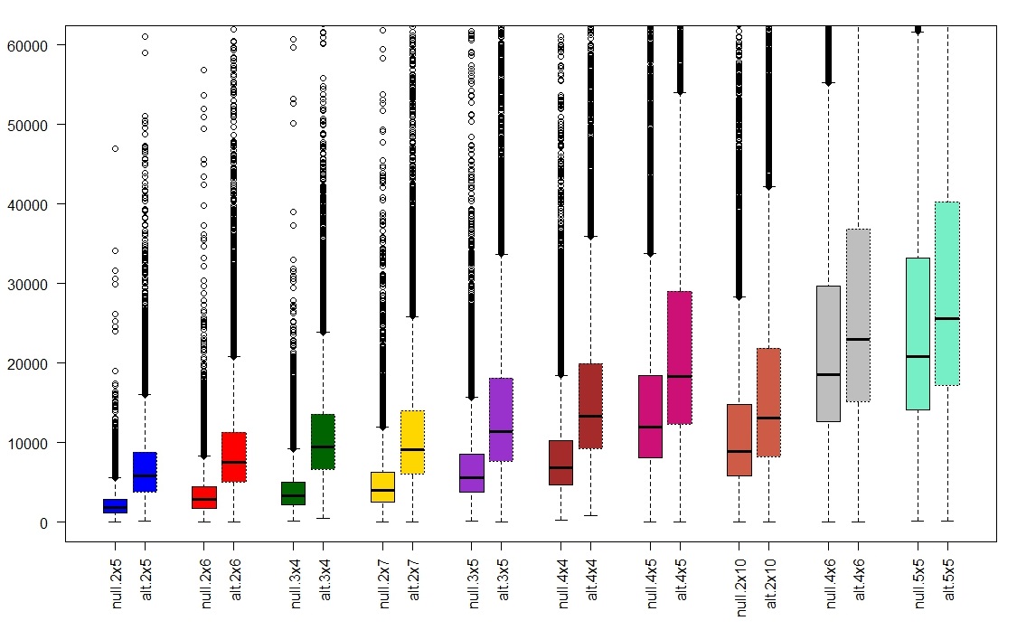 (d) 2-Dimensional Domains (12-30 types)
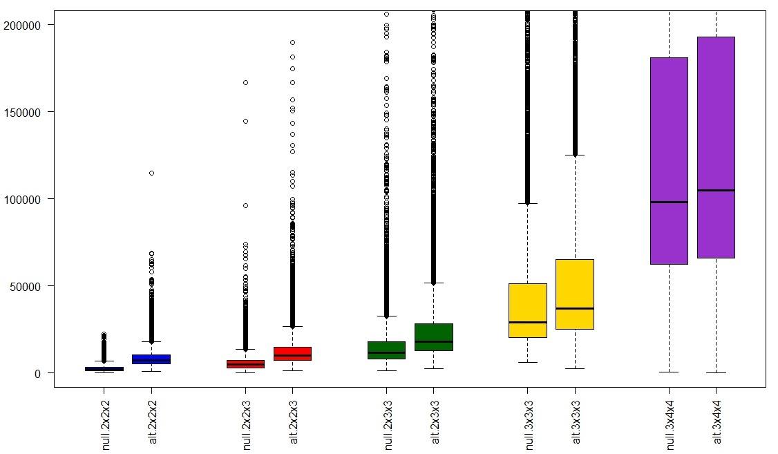 (e) 3-Dimensional Domains (8-48 types)
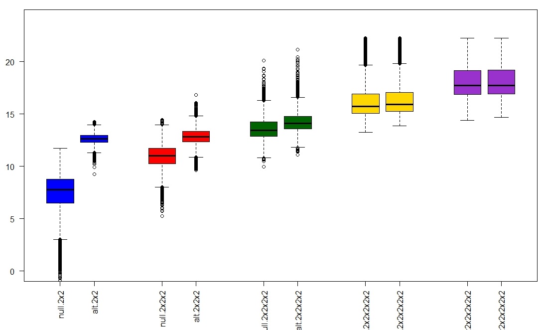 (f) Powers of 2 Size-Domains shown in log-scale (4-64 types)
|
(Best seen in color) We measured under both the null-hypothesis (solid line) and the alternative-hypothesis (dotted line) with various choices of domain sizes. As the size of the domain increases, it is evident the samples aren’t enough to differentiate between the null and the alternative. In all of the experiments and the alternative hypothesis is -far in TV-dist from a product distribution.