跳到论文正文
W Papers独立论文阅读器 arXiv:1802.03164 论文正文 计算阅读时间 · 0%
引用这篇论文根据当前论文元数据生成,正式投稿前建议核对。


License: arXiv.org perpetual non-exclusive license
arXiv:1802.03164v2 [math.AP] 03 Jun 2018

Global weak Besov solutions of the Navier-Stokes equations and applications

Dallas Albritton Note: School of Mathematics, University of Minnesota, Minneapolis, MN.
Email address: albri050@umn.edu
   Tobias Barker Note: OxPDE, Mathematical Institute, University of Oxford, Oxford, UK.
Email address: tobiasbarker5@gmail.com
August 24, 2026
Abstract

We introduce a notion of global weak solution to the Navier-Stokes equations in three dimensions with initial values in the critical homogeneous Besov spaces B˙p,∞−1+3p\dot{B}^{-1+\frac{3}{p}}_{p,\infty}, p>3p>3. These solutions satisfy a certain stability property with respect to the weak-∗\ast convergence of initial conditions. To illustrate this property, we provide applications to blow-up criteria, minimal blow-up initial data, and forward self-similar solutions. Our proof relies on a new splitting result in homogeneous Besov spaces that may be of independent interest.

1 Introduction

In this paper, we investigate certain classes of global-in-time weak solutions of the incompressible Navier-Stokes equations in three dimensions:

∂tv−Δ​v+v⋅∇v=−∇qdiv⁡v=0} in ℝ3×ℝ+.\left.\begin{aligned} \partial_{t}v-\Delta v+v\cdot\nabla v&=-\nabla q\\ \quad\div v&=0\end{aligned}\right\}\text{ in }\mathbb{R}^{3}\times\mathbb{R}_{+}. (NSE)

In the recent paper [47], G. Seregin and V. Šverák introduced a notion of global weak L3L^{3} solution to the Navier-Stokes equations which enjoys the following property. Given a sequence of global weak L3L^{3} solutions with initial data u0(n)⇀u0u_{0}^{(n)}\rightharpoonup u_{0} in L3L^{3}, there exists a subsequence converging in the sense of distributions to a global weak L3L^{3} solution with initial data u0u_{0}. This property, known as weak-∗\ast stability, plays a distinguished role in the regularity theory of the Navier-Stokes equations. For example, such sequences of solutions arise naturally when zooming in on a potential singularity of the Navier-Stokes equations, as in the papers [46, 48]11 1 In these papers, Seregin also investigated weak-∗\ast stability in the context of local Leray solutions, which were discovered by Lemarié-Rieusset [37]. by Seregin and [20] by Escauriaza, Seregin, and Šverák.

The main idea in [47] is to decompose a solution of the Navier-Stokes equations as

v=V+u,v=V+u, (1.1)

where VV is the linear evolution of the initial data u0∈L3u_{0}\in L^{3},

V⁡(x,t):=∫ℝ3Γ⁡(x−y,t)​u0​(y)​𝑑y,V(x,t):=\int_{\mathbb{R}^{3}}\Gamma(x-y,t)u_{0}(y)\,dy, (1.2)

and uu is a perturbation belonging to the global energy space

u∈Lt∞​Lx2∩Lt2​H˙x1​(QT)​ for all ​T>0.u\in L^{\infty}_{t}L^{2}_{x}\cap L^{2}_{t}\dot{H}^{1}_{x}(Q_{T})\text{ for all }T>0. (1.3)

Here, Γ:ℝ3×ℝ+→ℝ\Gamma\colon\mathbb{R}^{3}\times\mathbb{R}_{+}\to\mathbb{R} denotes the heat kernel in three dimensions, and

QT:=ℝ3×]0,T[,0<T≤∞,Q_{T}:=\mathbb{R}^{3}\times]0,T[,\quad 0<T\leq\infty, (1.4)

denotes a parabolic cylinder. It is reasonable to expect that solutions of the form v=V+uv=V+u enjoy weak-∗\ast stability, since the linear evolution VV is continuous in many nice topologies with respect to weak convergence of initial data, while the correction term uu is “merely a perturbation”.

In the paper [9], Barker et al. created a notion of global weak L3,∞L^{3,\infty} solution that contains the solutions in [47] as well as the scale-invariant solutions investigated by Jia and Šverák in [28] as a special case. These solutions exhibit some interesting phenomena. For instance, global weak L3,∞L^{3,\infty} solutions exist even when a local-in-time mild solution is not known to exist22 2 We mention that for divergence-free initial data in L3,∞L^{3,\infty} , there exists an associated global-in-time Lemarié-Rieusset local energy solution of the Navier-Stokes equations [37]. (unlike in the L3L^{3} case). It appears that such solutions may be non-unique even from the initial time, see the examples of the forward self-similar solutions computed by Guillod and Šverák in [25]. On the other hand, weak-∗\ast stability continues to hold in spite of the conjectured non-uniqueness. The authors of [9] also showed that global weak L3,∞L^{3,\infty} solutions provide a natural class in which to investigate minimal blow-up initial data. Šverák also mentioned the possibility of investigating the radius of smoothness (resp. uniqueness) associated to each initial data u0∈L3,∞u_{0}\in L^{3,\infty}. This is the maximal time such that each global weak L3L^{3} solution with prescribed initial data u0u_{0} is smooth (resp. unique).

Recently, the second author proposed in the paper [6] to investigate notions of solution in critical spaces XX that generalize the solutions described above. Namely, one desires a notion of global XX solution that satisfies a weak-∗\ast stability property when, for example,

X=H˙12,L3,L3,∞,B˙p,∞−1+3p,BMO−1,B˙∞,∞−1,3<p<∞.X=\dot{H}^{\frac{1}{2}},L^{3},L^{3,\infty},\dot{B}^{-1+\frac{3}{p}}_{p,\infty},{\rm BMO}^{-1},\dot{B}^{-1}_{\infty,\infty},\quad 3<p<\infty. (1.5)

The second author established the existence of global B˙4,∞−14\dot{B}^{-\frac{1}{4}}_{4,\infty} solutions with the decomposition v=V+uv=V+u utilized in previous works. Moreover, he proved that under natural hypotheses, B˙4,∞−14\dot{B}^{-\frac{1}{4}}_{4,\infty} is the largest critical space in which such a decomposition is viable. Therefore, a notion of global XX solution for the critical homogeneous Besov spaces X=B˙p,∞−1+3pX=\dot{B}^{-1+\frac{3}{p}}_{p,\infty} with 4<p<∞4<p<\infty must be based on a new structure.33 3 While critical spaces are not strictly necessary for weak-∗\ast stability (see p. 5 of the second author’s paper [7], for example), they are convenient for the applications we have in mind.

In this paper, we develop a notion of global weak Besov solution of the Navier-Stokes equations associated to initial data in the critical homogeneous Besov spaces B˙p,∞−1+3p​(ℝ3)\dot{B}^{-1+\frac{3}{p}}_{p,\infty}(\mathbb{R}^{3}), 3<p<∞3<p<\infty.

In Section 3, we prove the following results. Let 3<q≤p<∞3<q\leq p<\infty, and 0<T≤∞0<T\leq\infty. We include forcing terms of the form div⁡F\div F with F∈ℱq​(QT)F\in\mathcal{F}_{q}(Q_{T}), defined as the space of locally integrable functions F:QT→ℝ3×3F\colon Q_{T}\to\mathbb{R}^{3\times 3} such that

∥F∥ℱq​(QT):=supt∈]0,T[t1−32​q​∥F⁡(⋅,t)∥Lq​(ℝ3)<∞.\lVert F\rVert_{\mathcal{F}_{q}(Q_{T})}:=\sup_{t\in]0,T[}t^{1-\frac{3}{2q}}\lVert F(\cdot,t)\rVert_{L^{q}(\mathbb{R}^{3})}<\infty. (1.6)
Theorem 1.1 (Existence).

Let u0∈B˙p,∞−1+3p​(ℝ3)u_{0}\in\dot{B}^{-1+\frac{3}{p}}_{p,\infty}(\mathbb{R}^{3}) be a divergence-free vector field and F∈ℱq​(Q∞)F\in\mathcal{F}_{q}(Q_{\infty}). There exists a global weak Besov solution vv with initial data u0u_{0} and forcing term div⁡F\div F.

Theorem 1.2 (Weak–∗\ast stability).

Suppose that (v(n))n∈ℕ(v^{(n)})_{n\in\mathbb{N}} is a sequence of global weak Besov solutions with initial data u0(n)u_{0}^{(n)} and forcing terms div⁡F(n)\div F^{(n)}, respectively. Furthermore, suppose that

u0(n)​⇀∗​u0​ in ​B˙p,∞−1+3p​(ℝ3),F(n)​⇀∗​F​ in ​ℱq​(Q∞).u_{0}^{(n)}\overset{\ast}{\rightharpoonup}u_{0}\text{ in }\dot{B}^{-1+\frac{3}{p}}_{p,\infty}(\mathbb{R}^{3}),\quad F^{(n)}\overset{\ast}{\rightharpoonup}F\text{ in }\mathcal{F}_{q}(Q_{\infty}). (1.7)

Then there exists a subsequence converging strongly in Lloc3​(Q∞)L^{3}_{\rm loc}(Q_{\infty}) to a global weak Besov solution vv with initial data u0u_{0} and forcing term div⁡F\div F.

Theorem 1.3 (Weak-strong uniqueness).

There exists a constant ε0:=ε0​(p,q)>0\varepsilon_{0}:=\varepsilon_{0}(p,q)>0 such that for all u0∈B˙p,∞−1+3p​(ℝ3)u_{0}\in\dot{B}^{-1+\frac{3}{p}}_{p,\infty}(\mathbb{R}^{3}) divergence-free and F∈ℱq​(QT)F\in\mathcal{F}_{q}(Q_{T}) satisfying

∥u0∥B˙p,∞−1+3p​(ℝ3)+∥F∥ℱq​(QT)≤ε0,\lVert u_{0}\rVert_{\dot{B}^{-1+\frac{3}{p}}_{p,\infty}(\mathbb{R}^{3})}+\lVert F\rVert_{\mathcal{F}_{q}(Q_{T})}\leq\varepsilon_{0}, (1.8)

there exists a unique weak Besov solution on QTQ_{T} with initial data u0u_{0} and forcing term div⁡F\div F. This solution belongs to Lloc∞​(ℝ3×ℝ+)L^{\infty}_{\rm loc}(\mathbb{R}^{3}\times\mathbb{R}_{+}).

The second half of this paper is dedicated to applications of global weak Besov solutions. Namely, we provide applications to certain critical problems concerning blow-up criteria, minimal blow-up initial data, and forward self-similar solutions. We present these results at the end of the introduction. The reader interested only in applications is invited to skip to Section 1.1.

To motivate our notion of solution, it is instructive to write the perturbed Navier-Stokes system satisfied by the correction term in the decomposition v=V+uv=V+u used in the previous works [47, 9, 6]:

∂tu−Δ​u+(u+V)⋅∇u+u⋅∇V=−∇q−div⁡V⊗Vdiv⁡u=0} in ℝ3×ℝ+\left.\begin{aligned} \partial_{t}u-\Delta u+(u+V)\cdot\nabla u+u\cdot\nabla V&=-\nabla q-\div V\otimes V\\ \div u&=0\end{aligned}\right\}\text{ in }\mathbb{R}^{3}\times\mathbb{R}_{+} (1.9)

with zero initial condition. The associated global energy inequality is

‖u⁡(⋅,t)‖L22+2​∫0t∫ℝ3|∇u|2​𝑑x​d​t′≤2​∫0t∫ℝ3(V⊗u+V⊗V):∇u​𝑑x​d​t′.\|u(\cdot,t)\|_{L^{2}}^{2}+2\int\limits_{0}^{t}\int\limits_{\mathbb{R}^{3}}|\nabla u|^{2}\,dx\,dt^{\prime}\leq 2\int\limits_{0}^{t}\int\limits_{\mathbb{R}^{3}}(V\otimes u+V\otimes V):\nabla u\,dx\,dt^{\prime}. (1.10)

In order for the RHS of (1.10) to make sense, we require that

V∈Lt,loc4​Lx4​(ℝ3×ℝ+).V\in L^{4}_{t,{\rm loc}}L^{4}_{x}(\mathbb{R}^{3}\times\mathbb{R}_{+}). (1.11)

As demonstrated by the second author in [6], the quantitative scale-invariant version of (1.11) is ∥u0∥B˙4,∞−14≤M\lVert u_{0}\rVert_{\dot{B}^{-\frac{1}{4}}_{4,\infty}}\leq M, due to the caloric characterization of Besov spaces. Roughly speaking, the forcing term should belong to an L2L^{2}-based space, whereas V⊗VV\otimes V may only belong to spaces with integrability ≥p2\geq\frac{p}{2} for initial data u0∈B˙p,∞−1+3pu_{0}\in\dot{B}^{-1+\frac{3}{p}}_{p,\infty}. When p≫1p\gg 1, the obstacle is sometimes interpreted as “slow decay at spatial infinity.”

The notion of global weak Besov solution developed in this paper is based on the decomposition

v=Pk​(u0)+u,v=P_{k}(u_{0})+u, (1.12)

where Pk​(u0)P_{k}(u_{0}) is the kkth Picard iterate, k≥0k\geq 0, defined by

P0​(u0)​(⋅,t):=S⁡(t)​u0,P_{0}(u_{0})(\cdot,t):=S(t)u_{0}, (1.13)
Pk+1​(u0)​(⋅,t):=S⁡(t)​u0−B⁡(Pk,Pk),k≥0,P_{k+1}(u_{0})(\cdot,t):=S(t)u_{0}-B(P_{k},P_{k}),\quad k\geq 0, (1.14)

and BB is the bilinear term in the integral formulation of the Navier-Stokes equations (see (2.17) for the precise definition):

B⁡(u,v)​(⋅,t):=∫0tS⁡(t−s)​ℙ​div⁡u⊗v⁡(⋅,s)​𝑑s​𝑑x.B(u,v)(\cdot,t):=\int_{0}^{t}S(t-s)\mathbb{P}\div u\otimes v(\cdot,s)\,ds\,dx. (1.15)

The papers [47, 9, 6] utilized the decomposition (1.12) with k=0k=0. Observe that if vv solves (NSE), then u=v−Pku=v-P_{k} solves

∂tu−Δ​u+Pk⋅∇u+u⋅∇Pk+u⋅∇u=−∇p−div​Fkdiv⁡u=0} in ℝ3×ℝ+\left.\begin{aligned} \partial_{t}u-\Delta u+P_{k}\cdot\nabla u+u\cdot\nabla P_{k}+u\cdot\nabla u&=-\nabla p-\textrm{div}\,F_{k}\\ \div u&=0\end{aligned}\right\}\text{ in }\mathbb{R}^{3}\times\mathbb{R}_{+} (1.16)

with initial condition u⁡(⋅,0)=0u(\cdot,0)=0, where the forcing term Fk​(u0)F_{k}(u_{0}), k≥0k\geq 0, is defined by

Fk​(u0):=Pk⊗Pk−Pk−1⊗Pk−1,F_{k}(u_{0}):=P_{k}\otimes P_{k}-P_{k-1}\otimes P_{k-1}, (1.17)

and we use the convention that P−1​(u0)=0P_{-1}(u_{0})=0. One expects the correction uu to belong to the energy class if FkF_{k} belongs to L2​(ℝ3×]0,T[)L^{2}(\mathbb{R}^{3}\times]0,T[).

Here is our key observation:

Lemma 1.4 (Finite energy forcing).

Let p∈]3,∞[p\in]3,\infty[ and u0∈B˙p,∞−1+3p​(ℝ3)u_{0}\in\dot{B}^{-1+\frac{3}{p}}_{p,\infty}(\mathbb{R}^{3}) be a divergence-free vector field with ∥u0∥B˙p,∞−1+3p​(ℝ3)≤M\lVert u_{0}\rVert_{\dot{B}^{-1+\frac{3}{p}}_{p,\infty}(\mathbb{R}^{3})}\leq M. Then for all integers k≥k⁡(p):=⌈p2⌉−2k\geq k(p):=\lceil\frac{p}{2}\rceil-2, the forcing term Fk​(u0)F_{k}(u_{0}) satisfies

∥Fk​(u0)∥L2​(ℝ3×]0,T[)≤T14​C​(k,M,p).\lVert F_{k}(u_{0})\rVert_{L^{2}(\mathbb{R}^{3}\times]0,T[)}\leq T^{\frac{1}{4}}C(k,M,p). (1.18)

The proof of Lemma 1.4 is based on a self-improvement property of the bilinear term BB. Heuristically, if a vector field VV belongs to an LpL^{p}-based space, then B⁡(V,V)B(V,V) belongs to an Lp2L^{\frac{p}{2}}-based space (as well as the original space). For instance, let u0∈B˙6,∞−12​(ℝ3)u_{0}\in\dot{B}^{-\frac{1}{2}}_{6,\infty}(\mathbb{R}^{3}). Then V:=S​u0V:=Su_{0} belongs to an L6L^{6}-based space, and F1​(u0)F_{1}(u_{0}) satisfies

F1=−B(V,V)⊗V−V⊗B(V,V)+B(V,V)⊗B(V,V).F_{1}=-B(V,V)\otimes V-V\otimes B(V,V)+B(V,V)\otimes B(V,V). (1.19)

Since B⁡(V,V)B(V,V) belongs to an L3L^{3}-based space (and an L6L^{6}-based space), an application of Hölder’s inequality implies that F1F_{1} belongs to an L2L^{2}-based space. The same reasoning applies mutatis mutandis with the inclusion of a forcing term div⁡F\div F with FF belonging to ℱq​(QT)\mathcal{F}_{q}(Q_{T}) with q∈]3,p]q\in]3,p].44 4 See (1.6) or (2.18)-(2.19) for the relevant definition. The self-improvement property of BB was already exploited in the papers [22, 24]. The phenomenon that F1F_{1} is a higher order term is already present in the Picard iterates for the ODE x˙=a​x2\dot{x}=ax^{2}, x⁡(0)=x0x(0)=x_{0}, where a,x0∈ℝa,x_{0}\in\mathbb{R}.

Here is our main definition:

Definition 1.5 (Weak Besov solution).

Let T>0T>0, u0∈BMO−1​(ℝ3)u_{0}\in{\rm BMO}^{-1}(\mathbb{R}^{3}) be a divergence-free vector field, and F∈ℱ⁡(QT)F\in\mathcal{F}(Q_{T}).55 5 The requirements u0∈BMO−1​(ℝ3)u_{0}\in{\rm BMO}^{-1}(\mathbb{R}^{3}) and F∈ℱ⁡(QT)F\in\mathcal{F}(Q_{T}) ensure that the Picard iterates Pk​(u0,F)P_{k}(u_{0},F) are well-defined. We refer the reader to (2.10), (2.21), and (2.29)-(2.30) for the respective definitions.

We say that a distributional vector field vv on QT:=ℝ3×]0,T[Q_{T}:=\mathbb{R}^{3}\times]0,T[ is a weak Besov solution to the Navier-Stokes equations on QTQ_{T} with initial data u0u_{0} and forcing term div⁡F\div F if there exists an integer k≥0k\geq 0 such that the following requirements are satisfied.

First, there exists a pressure q∈Lloc32​(QT)q\in L^{\frac{3}{2}}_{\rm loc}(Q_{T}) such that vv satisfies the Navier-Stokes equations on QTQ_{T} in the sense of distributions:

∂tv−Δ​v+v⋅∇v=−∇q+div⁡F,div⁡v=0.\partial_{t}v-\Delta v+v\cdot\nabla v=-\nabla q+\div F,\qquad\div v=0. (1.20)

Second, vv may be decomposed as

v=u+Pk​(u0,F),v=u+P_{k}(u_{0},F), (1.21)

where u∈Lt∞​Lx2∩Lt2​H˙x1​(QT)u\in L^{\infty}_{t}L^{2}_{x}\cap L^{2}_{t}\dot{H}^{1}_{x}(Q_{T}) and u⁡(⋅,t)u(\cdot,t) is weakly L2L^{2}-continuous on [0,T][0,T]. Furthermore, we require that limt↓0∥u⁡(⋅,t)∥L2​(ℝ3)=0\lim_{t\downarrow 0}\lVert u(\cdot,t)\rVert_{L^{2}(\mathbb{R}^{3})}=0 and Fℓ∈L2​(QT)F_{\ell}\in L^{2}(Q_{T}) for all integers ℓ≥k\ell\geq k. Finally, we require that (v,q)(v,q) satisfies the following local energy inequality for every t∈]0,T[t\in]0,T[ and all non-negative test functions φ∈C0∞​(Q∞)\varphi\in C^{\infty}_{0}(Q_{\infty}):

∫ℝ3φ⁡(x,t)​|v⁡(x,t)|2​𝑑x+2​∫0t∫ℝ3φ​|∇v|2​𝑑x​d​t′\int_{\mathbb{R}^{3}}\varphi(x,t)|v(x,t)|^{2}\,dx+2\int_{0}^{t}\int_{\mathbb{R}^{3}}\varphi|\nabla v|^{2}\,dx\,dt^{\prime}
≤∫0t∫ℝ3|v|2​(∂tφ+Δ​φ)+v⁡(|v|2+2​q)⋅∇φ−2​F:∇(φ​v)​𝑑x​d​t′.\leq\int_{0}^{t}\int_{\mathbb{R}^{3}}|v|^{2}(\partial_{t}\varphi+\Delta\varphi)+v(|v|^{2}+2q)\cdot\nabla\varphi-2F:\nabla(\varphi v)\,dx\,dt^{\prime}. (1.22)

We say that the weak Besov solution is based on the kkth Picard iterate if the above properties are satisfied for a given integer k≥0k\geq 0.

We say that vv is a global weak Besov solution (or weak Besov solution on Q∞:=ℝ3×ℝ+Q_{\infty}:=\mathbb{R}^{3}\times\mathbb{R}_{+}) with initial data u0u_{0} and forcing term div⁡F\div F if there exists an integer k≥0k\geq 0 such that for all T>0T>0, vv is a weak Besov solution on QTQ_{T} based on the kkth Picard iterate with initial data u0u_{0} and forcing term div⁡F\div F.

Let us explain the requirement that Fℓ∈L2​(QT)F_{\ell}\in L^{2}(Q_{T}) for all ℓ≥k\ell\geq k. Its role is to ensure that vv is also a weak Besov solution based on the ℓ\ellth Picard iterate for all ℓ≥k\ell\geq k, see Proposition 3.4. In other words, one may always raise the order of the Picard iterate. Similarly, one may lower the Picard iterate depending on the regularity of the initial data. Hence, our notion of weak Besov solution in Definition 1.5 is not overly sensitive to the order of the Picard iterate.

Before turning to applications, we present another key ingredient in our arguments: a decay property for the correction term near the initial time.

Proposition 1.6 (Decay property).

Let p∈]3,∞[p\in]3,\infty[, q∈]3,p]q\in]3,p], and k≥k⁡(p):=⌈p2⌉−2k\geq k(p):=\lceil\frac{p}{2}\rceil-2. Assume that vv is a global weak Besov solution based on the kkth Picard iterate with initial data u0u_{0} and forcing term div⁡F\div F. Let ∥u0∥B˙p,∞−1+3p​(ℝ3)+∥F∥ℱq​(Q∞)≤M\lVert u_{0}\rVert_{\dot{B}^{-1+\frac{3}{p}}_{p,\infty}(\mathbb{R}^{3})}+\lVert F\rVert_{\mathcal{F}_{q}(Q_{\infty})}\leq M. Then

∥u⁡(⋅,t)∥L2​(ℝ3)≤C⁡(k,M,p,q)​t14.\lVert u(\cdot,t)\rVert_{L^{2}(\mathbb{R}^{3})}\leq C(k,M,p,q)t^{\frac{1}{4}}. (1.23)

The proof is given in Section 3.2. Notably, (1.23) is used to obtain the global energy inequality for the correction term starting from the initial time, see Corollary 3.9. A similar issue is already present in Seregin’s paper [49] for sequences of weak Leray-Hopf solutions with initial data converging to zero weakly in L2L^{2}.

To illustrate the main issue in Proposition 1.6, we consider the special case u0∈L3,∞u_{0}\in L^{3,\infty} with zero forcing term and decompose the solution as v=V+uv=V+u as in the paper [9]. That is, k=0k=0 in Definition 1.5. Heuristically, the energy of the correction term should originate entirely in the forcing term −divV⊗V-\div V\otimes V. Let ∥u0∥L3,∞≤M\lVert u_{0}\rVert_{L^{3,\infty}}\leq M. Since

∫ℝ3∫0t|V⊗V|2​𝑑x​𝑑t≤C​t12​M2​ for all ​t>0,\int_{\mathbb{R}^{3}}\int_{0}^{t}|V\otimes V|^{2}\,dx\,dt\leq Ct^{\frac{1}{2}}M^{2}\text{ for all }t>0, (1.24)

we expect the following a priori estimate:

‖u⁡(⋅,t)‖L22+2​∫0t∫ℝ3|∇u|2​𝑑x​d​t′≤t12​C​(M).\|u(\cdot,t)\|_{L^{2}}^{2}+2\int\limits_{0}^{t}\int\limits_{\mathbb{R}^{3}}|\nabla u|^{2}\,dx\,dt^{\prime}\leq t^{\frac{1}{2}}C(M). (1.25)

When u0∈L3u_{0}\in L^{3}, the proof of (1.25) is via a Gronwall-type argument that does not extend to the more general case. For instance, consider the following estimate for the lower order term in the global energy inequality:

|∫0T∫ℝ3V⊗u:∇udxdt′|≤C∥V∥Lt∞​Lx3,∞​(QT)∥u∥Lt2​Lx6,2​(QT)∥∇u∥L2​(QT),\left\lvert\int_{0}^{T}\int_{\mathbb{R}^{3}}V\otimes u:\nabla u\,dx\,dt^{\prime}\right\rvert\leq C\lVert V\rVert_{L^{\infty}_{t}L^{3,\infty}_{x}(Q_{T})}\lVert u\rVert_{L^{2}_{t}L^{6,2}_{x}(Q_{T})}\lVert\nabla u\rVert_{L^{2}(Q_{T})}, (1.26)

where the quantity ∥V∥Lt∞​Lx3,∞​(QT)\lVert V\rVert_{L^{\infty}_{t}L^{3,\infty}_{x}(Q_{T})} is not “locally small” unless M≪1M\ll 1.

In the paper [9], this issue is overcome using splitting arguments66 6 Related splitting arguments have also previously been used by Jia and Šverák in [27], in order to show estimates near the initial time for Lemarié-Rieusset local energy solutions of the Navier-Stokes equations with L3L^{3} initial data. inspired by C. P. Calderón [15] and a decomposition of initial data in Lorentz spaces. In the present work, we require the following new decomposition of initial data in Besov spaces.77 7 This lemma was obtained by the second author in [6, Proposition 1.5], which will not be submitted for journal publication.

Lemma 1.7 (Splitting of initial data).

Let p∈]d,∞[p\in]d,\infty[. There exist p2∈]p,∞[p_{2}\in]p,\infty[, δ2∈]0,−sp2[\delta_{2}\in]0,-s_{p_{2}}[, γ1,γ2>0\gamma_{1},\gamma_{2}>0, and C>0C>0, each depending only on pp, such that for each divergence-free vector field g∈B˙p,∞sp​(ℝd)g\in\dot{B}^{s_{p}}_{p,\infty}(\mathbb{R}^{d}) and N>0N>0, there exist divergence-free vector fields g¯N∈B˙p2,p2sp2+δ2​(ℝd)∩B˙p,∞sp​(ℝd)\bar{g}^{N}\in\dot{B}^{s_{p_{2}}+\delta_{2}}_{p_{2},p_{2}}(\mathbb{R}^{d})\cap\dot{B}^{s_{p}}_{p,\infty}(\mathbb{R}^{d}) and g~N∈L2​(ℝd)∩B˙p,∞sp​(ℝd)\widetilde{g}^{N}\in L^{2}(\mathbb{R}^{d})\cap\dot{B}^{s_{p}}_{p,\infty}(\mathbb{R}^{d}) with the following properties:

g=g~N+g¯N,g=\widetilde{g}^{N}+\bar{g}^{N}, (1.27)
‖g~N‖L2​(ℝd)≤C​N−γ2​∥g∥B˙p,∞sp​(ℝd),\|\widetilde{g}^{N}\|_{L^{2}(\mathbb{R}^{d})}\leq CN^{-\gamma_{2}}\lVert g\rVert_{\dot{B}^{s_{p}}_{p,\infty}(\mathbb{R}^{d})}, (1.28)
‖g¯N‖B˙p2,p2sp2+δ2​(ℝd)≤C​Nγ1​∥g∥B˙p,∞sp​(ℝd).\|\bar{g}^{N}\|_{\dot{B}^{s_{p_{2}}+\delta_{2}}_{p_{2},p_{2}}(\mathbb{R}^{d})}\leq CN^{\gamma_{1}}\lVert g\rVert_{\dot{B}^{s_{p}}_{p,\infty}(\mathbb{R}^{d})}. (1.29)

Furthermore,

‖g~N‖B˙p,∞sp​(ℝd),‖g¯N‖B˙p,∞sp​(ℝd)≤C​∥g∥B˙p,∞sp​(ℝd).\|\widetilde{g}^{N}\|_{\dot{B}^{s_{p}}_{p,\infty}(\mathbb{R}^{d})},\|\bar{g}^{N}\|_{\dot{B}^{s_{p}}_{p,\infty}(\mathbb{R}^{d})}\leq C\lVert g\rVert_{\dot{B}^{s_{p}}_{p,\infty}(\mathbb{R}^{d})}. (1.30)

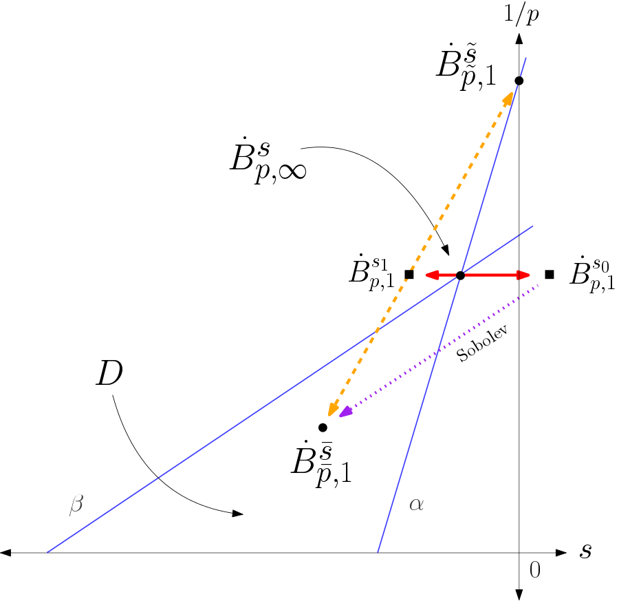
The most notable feature of Lemma 1.7 is that the summability index qq is reduced from ∞\infty in both terms of the decomposition. Therefore, the splitting is not a simple “diagonal splitting” that could be obtained via complex interpolation of Besov spaces. Moreover, it does not appear to obviously follow from the abstract real interpolation theory, since Besov spaces are not real interpolation spaces of Besov spaces except in special cases (such as when the integrability index pp is kept constant), see [35, Section 4] for an example. Further discussion and the proof of a general splitting result, Proposition 5.6, are contained in Section 5.

Refer to caption
Figure 1.8: Illustration of Lemma 1.7 with d=3d=3. The initial data g∈B˙p,∞spg\in\dot{B}^{s_{p}}_{p,\infty} is split along the dashed red lines into g~∈L2\widetilde{g}\in L^{2} and g¯∈B˙p2,p2sp2+δ2\bar{g}\in\dot{B}^{s_{p_{2}}+\delta_{2}}_{p_{2},p_{2}}.

1.1 Applications

The second part of the paper is focused on applications of global weak Besov solutions to three problems concerning the three-dimensional Navier-Stokes equations.

1.1.1 Blow-up criteria

Our first application is an improved blow-up criterion for the Navier-Stokes equations in critical spaces:

Corollary 1.9 (B˙p,∞−1+3p\dot{B}^{-1+\frac{3}{p}}_{p,\infty} blow-up criterion).

Let T∗>0T^{*}>0, u0∈L∞​(ℝ3)u_{0}\in L^{\infty}(\mathbb{R}^{3}) be a divergence-free vector field, and F∈Lt∞​Lxq​(ℝ3×]0,T∗[)F\in L^{\infty}_{t}L^{q}_{x}(\mathbb{R}^{3}\times]0,T^{*}[) for some q∈]3,∞[q\in]3,\infty[. Suppose that v∈L∞​(ℝ3×]0,T[)v\in L^{\infty}(\mathbb{R}^{3}\times]0,T[) is a mild solution of the Navier-Stokes equations on ℝ3×]0,T[\mathbb{R}^{3}\times]0,T[ with initial data u0u_{0} and forcing term div⁡F\div F for all T∈]0,T∗[T\in]0,T^{*}[. Suppose that there exists a sequence of times tn↑T∗t_{n}\uparrow T^{*} such that

supn∈ℕ∥v⁡(⋅,tn)∥B˙p,∞−1+3p​(ℝ3)<∞\sup_{n\in\mathbb{N}}\lVert v(\cdot,t_{n})\rVert_{\dot{B}^{-1+\frac{3}{p}}_{p,\infty}(\mathbb{R}^{3})}<\infty (1.31)

for some p∈]3,∞[p\in]3,\infty[. Finally, assume that v⁡(⋅,T∗)v(\cdot,T^{*}) satisfies

T∗−tnv(T∗−tn(⋅−x∗),T∗)⇀∗0 in 𝒟′(ℝ3),\sqrt{T^{*}-t_{n}}v(\sqrt{T^{*}-t_{n}}(\cdot-x^{*}),T^{*})\overset{\ast}{\rightharpoonup}0\text{ in }\mathcal{D}^{\prime}(\mathbb{R}^{3}), (1.32)

for some x∗∈ℝ3x^{*}\in\mathbb{R}^{3}. Then vv is regular at (x∗,T∗)(x^{*},T^{*}).88 8 We say that vv is regular at (x∗,T∗)∈ℝ3+1(x^{*},T^{*})\in\mathbb{R}^{3+1} if v∈L∞(B(x∗,R)×]T∗−R2,T∗[)v\in L^{\infty}(B(x^{*},R)\times]T^{*}-R^{2},T^{*}[) for some R>0R>0. Otherwise, it is singular at (x∗,T∗)(x^{*},T^{*}). If (1.32) is verified for all x∗∈ℝ3x^{*}\in\mathbb{R}^{3}, then v∈L∞​(ℝ3×]0,T∗[)v\in L^{\infty}(\mathbb{R}^{3}\times]0,T^{*}[).

Corollary 1.9 is a special case of Theorem 4.1, which may be regarded as a quantitative version of the corollary. For comparison, the following weaker criterion was obtained without forcing term by the first author in [1]:

limt↑T∗∥v⁡(⋅,t)∥B˙p,q−1+3p​(ℝ3)=∞​ with ​p,q∈]3,∞[.\lim_{t\uparrow T^{*}}\lVert v(\cdot,t)\rVert_{\dot{B}^{-1+\frac{3}{p}}_{p,q}(\mathbb{R}^{3})}=\infty\text{ with }p,q\in]3,\infty[. (1.33)

We also mention the preceding works [20, 48, 46, 42, 8, 31, 23, 24] in this direction.99 9 Corollary 1.9 without forcing term appeared in the recent preprint [6] of the second author which is not intended to be submitted for publication. Specifically, our methods are based on the rescaling procedure and backward uniqueness arguments introduced by Escauriaza, Seregin, and Šverák in [20] and further developed by Seregin in [48, 46].

The requirement (1.32) states that the blow-up profile v⁡(⋅,T∗)v(\cdot,T^{*}) vanishes in the limit of the rescaling procedure. This assumption excludes, for example, the situation that v⁡(⋅,T∗)v(\cdot,T^{*}) is scale-invariant, in which case zooming on the singularity would provide no new information. If v⁡(⋅,T∗)v(\cdot,T^{*}) belongs to the closure of Schwartz functions in B˙∞,∞−1​(ℝ3)\dot{B}^{-1}_{\infty,\infty}(\mathbb{R}^{3}), then (1.32) is automatically satisfied. See Section 4.1 for further remarks.

The reason for the restriction q>3q>3 on the forcing term is to ensure that the maximal time of existence is indicated by the formation of a singularity. Note, for instance, that solutions of the equation Δ​u=div⁡F\Delta u=\div F in ℝd\mathbb{R}^{d} with FF belonging to Ld​(ℝd)L^{d}(\mathbb{R}^{d}) may not be locally bounded when d≥2d\geq 2.

Finally, let us mention that the “concentration+rigidity” roadmap of Kenig and Merle [32] was utilised by Koch and Kenig in [31], and subsequently by Koch, Gallagher and Planchon in [23]-[24] to show the following. Namely, if the maximal time of existence Tmax​(u0)T_{\rm max}(u_{0}) is finite, then

lim supt↑Tmax​(u0)∥v⁡(⋅,t)∥X=∞\limsup_{t\uparrow T_{\rm max}(u_{0})}\lVert v(\cdot,t)\rVert_{X}=\infty (1.34)

for X=H˙12​(ℝ3)X=\dot{H}^{\frac{1}{2}}(\mathbb{R}^{3}) [31], L3​(ℝ3)L^{3}(\mathbb{R}^{3})[23]1010 10 The result for L3​(ℝ3)L_{3}(\mathbb{R}^{3}) and H˙12​(ℝ3)\dot{H}^{\frac{1}{2}}(\mathbb{R}^{3}) was first obtained in [20]., and B˙p,q−1+3p​(ℝ3)\dot{B}^{-1+\frac{3}{p}}_{p,q}(\mathbb{R}^{3}) (3<p,q<∞3<p,q<\infty) [24]. The approach of the aforementioned papers relies on profile decompositions of sequences of elements bounded in the above spaces XX. In [5, Remark 3.1], it is conjectured that profile decompositions fail for the continuous embedding B˙p,∞−1+3p​(ℝ3)↪B˙p′,∞−1+3p′​(ℝ3)\dot{B}^{-1+\frac{3}{p}}_{p,\infty}(\mathbb{R}^{3})\hookrightarrow\dot{B}^{-1+\frac{3}{p^{\prime}}}_{p^{\prime},\infty}(\mathbb{R}^{3}) (3<p≤p′3<p\leq p^{{}^{\prime}}). Thus, it seems challenging to use the approach in [31] and [24]-[23] to obtain Corollary 1.9.

1.1.2 Minimal blow-up problems

Our second application is to minimal blow-up questions in the context of global weak Besov solutions. The existence of minimal blow-up initial data was first proven by Rusin and Šverák in [45] in the class of mild solutions with initial data belonging to H˙12\dot{H}^{\frac{1}{2}} (provided that such solutions may form singularities in finite time). Analogous results were established for L3L^{3} by Jia and Šverák in [27] and for B˙p,q−1+3p\dot{B}^{-1+\frac{3}{p}}_{p,q}, p,q∈]3,∞[p,q\in]3,\infty[ by Gallagher, G. Koch, and Planchon in [24].

While local-in-time mild solutions are not known to exist for each solenoidal initial data in L3,∞L^{3,\infty} or B˙p,∞−1+3p\dot{B}^{-1+\frac{3}{p}}_{p,\infty}, the minimal blow-up data problem in these spaces may be reformulated for certain classes of weak solutions. This was originally observed by the second author, Seregin, and Šverák in [9] for global weak L3,∞L^{3,\infty} solutions. We now formulate the problem for global weak Besov solutions:

Definition 1.10 (Critical space).

Let (𝒳,∥⋅∥𝒳)(\mathcal{X},\lVert\cdot\rVert_{\mathcal{X}}) be a Banach space consisting of divergence-free distributional vector fields on ℝ3\mathbb{R}^{3}. We say that 𝒳\mathcal{X} is a critical space provided that

  1. (i)

    𝒳\mathcal{X} is continuously embedded in B˙∞,∞−1​(ℝ3)\dot{B}^{-1}_{\infty,\infty}(\mathbb{R}^{3}),

  2. (ii)

    𝒳\mathcal{X} and ∥⋅∥𝒳\lVert\cdot\rVert_{\mathcal{X}} are invariant under spatial translation and the scaling symmetry of the Navier-Stokes equations, and

  3. (iii)

    B¯𝒳:={u0∈𝒳:∥u0∥𝒳≤1}\bar{B}^{\mathcal{X}}:=\{u_{0}\in\mathcal{X}:\lVert u_{0}\rVert_{\mathcal{X}}\leq 1\} is sequentially compact in the topology of distributions.

Let 𝒳\mathcal{X} be a critical space which is embedded into B˙p,∞−1+3p​(ℝ3)\dot{B}^{-1+\frac{3}{p}}_{p,\infty}(\mathbb{R}^{3}) for some p∈]3,∞[p\in]3,\infty[. By Theorem 1.3, there exists ρ>0\rho>0 satisfying

  • (small data implies smooth) u0∈𝒳u_{0}\in\mathcal{X} and ‖u0‖𝒳<ρ\|u_{0}\|_{\mathcal{X}}<\rho implies that any global weak Besov solution with initial data u0u_{0} has no singular points

Then the following quantity is well defined:

  • ρ𝒳:=sup({ρ>0:\rho_{\mathcal{X}}:=\sup(\{\rho>0: for all u0∈𝒳u_{0}\in\mathcal{X} satisfying ∥u0∥𝒳≤ρ\lVert u_{0}\rVert_{\mathcal{X}}\leq\rho, any global weak Besov solution with initial condition u0u_{0} has no singular points})\}).

Under the assumption that ρ𝒳<∞\rho_{\mathcal{X}}<\infty, one may ask whether the above supremum is attained: Does there exist a global weak Besov solution v~\widetilde{v} with initial data u~0∈𝒳\widetilde{u}_{0}\in\mathcal{X} such that v~\widetilde{v} has a singular point and ‖u~0‖𝒳=ρ𝒳\|\widetilde{u}_{0}\|_{\mathcal{X}}=\rho_{\mathcal{X}}? Such u0~\widetilde{u_{0}} is referred to as minimal blow-up initial data. We answer this question in the affirmative below:

Corollary 1.11 (Minimal blow-up data).

Let 𝒳\mathcal{X} be a critical space continuously embedded into B˙p,∞−1+3p​(ℝ3)\dot{B}^{-1+\frac{3}{p}}_{p,\infty}(\mathbb{R}^{3}) for some p∈]3,∞[p\in]3,\infty[. Suppose that ρ𝒳<∞\rho_{\mathcal{X}}<\infty. Then there exists a solenoidal vector field u0~∈𝒳\widetilde{u_{0}}\in\mathcal{X} with ∥u0~∥𝒳=ρ𝒳\lVert\widetilde{u_{0}}\rVert_{\mathcal{X}}=\rho_{\mathcal{X}} such that u0~\widetilde{u_{0}} is initial data for a singular global weak Besov solution. The set of such u0~\widetilde{u_{0}} is sequentially compact (modulo spatial translation and the scaling symmetry of the Navier-Stokes equations) in the topology of distributions.

Our more general result is Theorem 4.7, which treats the problem of minimal blow-up perturbations of global solutions, thus generalizing the work [44] of Rusin for H˙12\dot{H}^{\frac{1}{2}} initial data. On the other hand, Corollary 1.11 already contains the previously known results for 𝒳=H˙12,L3\mathcal{X}=\dot{H}^{\frac{1}{2}},L^{3}, and B˙p,q−1+3p\dot{B}^{-1+\frac{3}{p}}_{p,q} with p,q∈]3,∞[p,q\in]3,\infty[ due to weak-strong uniqueness for global weak Besov solutions. While Corollary 1.11 only asserts the sequential compactness in the topology of distributions, we may upgrade to convergence in norm if the critical space is uniformly convex, as in the examples above. For 𝒳=B˙p,∞−1+3p\mathcal{X}=\dot{B}^{-1+\frac{3}{p}}_{p,\infty}, compactness is in the weak-∗\ast topology. A minor point is that our approach also accounts for any possible changes in the set of minimal blow-up initial data under renormings of the critical space.

1.1.3 Self-similar solutions

Our final application concerns forward-in-time self-similar solutions of the Navier-Stokes equations. A locally integrable vector field v:ℝ3×ℝ+→ℝ3v\colon\mathbb{R}^{3}\times\mathbb{R}_{+}\to\mathbb{R}^{3} is discretely self-similar with scaling factor λ>1\lambda>1 (λ\lambda-DSS) provided that

v⁡(x,t)=λ​v​(λ​x,λ2​t)​ for a.e. ​(x,t)∈ℝ3×ℝ+.v(x,t)=\lambda v(\lambda x,\lambda^{2}t)\text{ for a.e. }(x,t)\in\mathbb{R}^{3}\times\mathbb{R}_{+}. (1.35)

The vector field is self-similar (scale-invariant) if the relation (1.35) is verified for all λ>0\lambda>0. We consider also the analogous definition for vector fields on ℝ3\mathbb{R}^{3} and for distributional vector fields.

Although self-similar solutions of the Navier-Stokes equations have a rich history going back to Leray [39]1111 11 In [39], Leray posed the question of whether backward self-similar solutions of the Navier-Stokes equations exist. These were subsequently ruled out in [41] and [53]., the existence of large-data forward self-similar solutions was settled only recently by Jia and Šverák in [28]. These solutions have important consequences for the potential non-uniqueness of weak Leray-Hopf solutions, as investigated in [29, 25]. While the solutions in [28] correspond to scale-invariant data in Clocα​(ℝ3∖{0})C^{\alpha}_{\rm loc}(\mathbb{R}^{3}\setminus\{0\}), there is also an abundant literature on the existence of (discretely) self-similar solutions evolving from rough initial data [54, 34, 12, 38, 13, 11, 17]. In particular, we are interested in the paper [11] of Bradshaw and Tsai, which established the existence of discretely self-similar solutions associated to initial data u0∈B˙p,∞−1+3p​(ℝ3)u_{0}\in\dot{B}^{-1+\frac{3}{p}}_{p,\infty}(\mathbb{R}^{3}), p∈]3,6[p\in]3,6[. Our final application is the following extension of their work:

Theorem 1.12 (Existence of (discretely) self-similar solutions).

Suppose u0∈B˙p,∞−1+3p​(ℝ3)u_{0}\in\dot{B}^{-1+\frac{3}{p}}_{p,\infty}(\mathbb{R}^{3}) is a divergence-free vector field for some p∈]3,∞[p\in]3,\infty[. If u0u_{0} is λ\lambda–DSS for some scaling factor λ>1\lambda>1, then there exists a λ\lambda–DSS global weak Besov solution with initial data u0u_{0}. If u0u_{0} is scale-invariant, then there exists a scale-invariant global weak Besov solution with initial data u0u_{0}.

To prove Theorem 1.12, we approximate u0∈B˙p,∞−1+3p​(ℝ3)u_{0}\in\dot{B}^{-1+\frac{3}{p}}_{p,\infty}(\mathbb{R}^{3}) by a sequence of (discretely) self-similar initial data belonging to the Lorentz space L3,∞​(ℝ3)L^{3,\infty}(\mathbb{R}^{3}). The proof is completed by applying the weak-∗\ast stability property to an associated sequence of (discretely) self-similar solutions whose existence was established in [12].

2 Preliminaries

2.1 Function spaces

Let d,m∈ℕd,m\in\mathbb{N}. We begin by recalling the definition of the homogeneous Besov spaces B˙p,qs​(ℝd,ℝm)\dot{B}^{s}_{p,q}(\mathbb{R}^{d};\mathbb{R}^{m}). Our treatment follows [4, Chapter 2]. There exists a non-negative radial function φ∈C∞​(ℝd)\varphi\in C^{\infty}(\mathbb{R}^{d}) supported on the annulus {ξ∈ℝd:3/4≤|ξ|≤8/3}\{\xi\in\mathbb{R}^{d}:3/4\leq|\xi|\leq 8/3\} such that

∑j∈ℤφ⁡(2−j​ξ)=1,ξ∈ℝ3∖{0}.\sum_{j\in\mathbb{Z}}\varphi(2^{-j}\xi)=1,\quad\xi\in\mathbb{R}^{3}\setminus\{0\}. (2.1)

The homogeneous Littlewood-Paley projectors Δ˙j\dot{\Delta}_{j} are defined by

Δ˙j​f=φ⁡(2−j​D)​f,j∈ℤ,\dot{\Delta}_{j}f=\varphi(2^{-j}D)f,\quad j\in\mathbb{Z}, (2.2)

for all tempered distributions ff on ℝd\mathbb{R}^{d} with values in ℝm\mathbb{R}^{m}. The notation φ⁡(2−j​D)​f\varphi(2^{-j}D)f denotes convolution with the inverse Fourier transform of φ(2−j⋅)\varphi(2^{-j}\cdot) with ff.

Let p,q∈[1,∞]p,q\in[1,\infty] and s∈]−∞,d/p[s\in]-\infty,d/p[.1212 12 The choice s=d/ps=d/p, q=1q=1 is also valid. The homogeneous Besov space B˙p,qs​(ℝd,ℝm)\dot{B}^{s}_{p,q}(\mathbb{R}^{d};\mathbb{R}^{m}) consists of all tempered distributions ff on ℝd\mathbb{R}^{d} with values in ℝm\mathbb{R}^{m} satisfying

∥f∥B˙p,qs​(ℝd,ℝm):=‖(2j​s​∥Δ˙j​f∥Lp)j∈ℤ‖ℓq<∞\lVert f\rVert_{\dot{B}^{s}_{p,q}(\mathbb{R}^{d};\mathbb{R}^{m})}:=\left\lVert\big(2^{js}\lVert\dot{\Delta}_{j}f\rVert_{L^{p}}\big)_{j\in\mathbb{Z}}\right\rVert_{\ell^{q}}<\infty (2.3)

and such that ∑j∈ℤΔ˙j​f\sum_{j\in\mathbb{Z}}\dot{\Delta}_{j}f converges to ff in the sense of tempered distributions on ℝd\mathbb{R}^{d} with values in ℝm\mathbb{R}^{m}. In this range of indices, B˙p,qs​(ℝd,ℝm)\dot{B}^{s}_{p,q}(\mathbb{R}^{d};\mathbb{R}^{m}) is a Banach space. When s≥3/ps\geq 3/p and q>1q>1, the spaces must be considered modulo polynomials, see Section 5. Note that other reasonable choices of the function φ\varphi defining Δ˙j\dot{\Delta}_{j} lead to equivalent norms. In general, Besov spaces may also be characterized as real interpolation spaces of Bessel potential spaces, see [10, 37]. For now, we only consider d=m=3d=m=3.

We now recall a particularly useful property of Besov spaces, i.e., their characterization in terms of the heat kernel. For all s∈]−∞,0[s\in]-\infty,0[, there exists a constant c:=c⁡(s)>0c:=c(s)>0 such that for all tempered distributions ff on ℝ3\mathbb{R}^{3},

c−1​supt>0t−s2​∥S⁡(t)​f∥Lp​(ℝ3)≤∥f∥B˙p,∞s​(ℝ3)≤c​supt>0t−s2​∥S⁡(t)​f∥Lp​(ℝ3),c^{-1}\sup_{t>0}t^{-\frac{s}{2}}\lVert S(t)f\rVert_{L^{p}(\mathbb{R}^{3})}\leq\lVert f\rVert_{\dot{B}^{s}_{p,\infty}(\mathbb{R}^{3})}\leq c\sup_{t>0}t^{-\frac{s}{2}}\lVert S(t)f\rVert_{L^{p}(\mathbb{R}^{3})}, (2.4)

where we use the notation

(S​f)​(⋅,t)=S⁡(t)​f=Γ⁡(⋅,t)∗f,t>0,(Sf)(\cdot,t)=S(t)f=\Gamma(\cdot,t)\ast f,\quad t>0, (2.5)

and Γ:ℝ3×ℝ+→ℝ\Gamma\colon\mathbb{R}^{3}\times\mathbb{R}_{+}\to\mathbb{R} is the heat kernel in three dimensions. This motivates the definition of the Kato spaces 𝒦ps​(QT)\mathcal{K}^{s}_{p}(Q_{T}) with parameters s∈ℝs\in\mathbb{R}, p∈[1,∞]p\in[1,\infty], and 0<T≤∞0<T\leq\infty. The Kato spaces consist of all locally integrable vector fields u:QT→ℝ3u\colon Q_{T}\to\mathbb{R}^{3} satisfying

∥u∥𝒦ps​(QT):=ess​supt∈]0,T[⁡t−s2​∥u⁡(⋅,t)∥Lp​(ℝ3)<∞.\lVert u\rVert_{\mathcal{K}^{s}_{p}(Q_{T})}:=\esssup_{t\in]0,T[}t^{-\frac{s}{2}}\lVert u(\cdot,t)\rVert_{L^{p}(\mathbb{R}^{3})}<\infty. (2.6)

We abbreviate

𝒦p​(QT):=𝒦psp​(QT),sp:=−1+3/p.\mathcal{K}_{p}(Q_{T}):=\mathcal{K}^{s_{p}}_{p}(Q_{T}),\quad s_{p}:=-1+3/p. (2.7)

Therefore, for all p∈]3,∞]p\in]3,\infty], there exists a constant c:=c⁡(p)>0c:=c(p)>0 such that

c−1​∥S​u0∥𝒦p​(Q∞)≤∥u0∥B˙p,∞sp​(ℝ3)≤c​∥S​u0∥𝒦p​(Q∞),c^{-1}\lVert Su_{0}\rVert_{\mathcal{K}_{p}(Q_{\infty})}\leq\lVert u_{0}\rVert_{\dot{B}^{s_{p}}_{p,\infty}(\mathbb{R}^{3})}\leq c\lVert Su_{0}\rVert_{\mathcal{K}_{p}(Q_{\infty})}, (2.8)

for all vector fields u0∈B˙p,∞sp​(ℝ3)u_{0}\in\dot{B}^{s_{p}}_{p,\infty}(\mathbb{R}^{3}). As demonstrated in [16] and [43], the characterization (2.8) is particularly well suited for constructing mild solutions of the Navier-Stokes equations.

Next, for all 0<T≤∞0<T\leq\infty, consider the space 𝒳T\mathcal{X}_{T} consisting of all locally integrable functions uu on QTQ_{T} such that

∥u∥𝒳T:=ess​supt∈]0,T[⁡t12​∥u⁡(⋅,t)∥L∞​(ℝ3)+supx∈ℝ3supR∈]0,T[R−32​∥u∥L2​(B⁡(x,R)×]0,R2[)<∞.\lVert u\rVert_{\mathcal{X}_{T}}:=\esssup_{t\in]0,T[}t^{\frac{1}{2}}\lVert u(\cdot,t)\rVert_{L^{\infty}(\mathbb{R}^{3})}+\sup_{x\in\mathbb{R}^{3}}\sup_{R\in]0,\sqrt{T}[}R^{-\frac{3}{2}}\lVert u\rVert_{L^{2}(B(x,R)\times]0,R^{2}[)}<\infty. (2.9)

This is the largest space on which the bilinear operator BB is known to be bounded, see the paper [33] of H. Koch and D. Tataru. We use the following Carleson measure characterization of ∥⋅∥BMO−1​(ℝ3)\lVert\cdot\rVert_{{\rm BMO}^{-1}(\mathbb{R}^{3})}. Namely, for all tempered distributions ff on ℝ3\mathbb{R}^{3}, we define

∥f∥BMO−1​(ℝ3):=∥S​f∥𝒳∞.\lVert f\rVert_{{\rm BMO}^{-1}(\mathbb{R}^{3})}:=\lVert Sf\rVert_{\mathcal{X}_{\infty}}. (2.10)

The space BMO−1​(ℝ3){\rm BMO}^{-1}(\mathbb{R}^{3}) consists of all tempered distributions on ℝ3\mathbb{R}^{3} with finite BMO−1{\rm BMO}^{-1} norm.

Let us clarify the relationships between various function spaces of initial data. The Lorentz space L3,∞​(ℝ3)L^{3,\infty}(\mathbb{R}^{3}) is continuously embedded into B˙p,∞sp​(ℝ3)\dot{B}^{s_{p}}_{p,\infty}(\mathbb{R}^{3}) for all p∈]3,∞]p\in]3,\infty]. This may be proven using (2.4) and Young’s convolution inequality for Lorentz spaces. Next, the Bernstein inequalities for frequency-localized functions imply an analogue of the Sobolev embedding theorem for homogeneous Besov spaces. Finally, regarding BMO−1​(ℝ3){\rm BMO}^{-1}(\mathbb{R}^{3}), Hölder’s inequality gives

supx∈ℝ3supR>0R−32​∥S⁡(t)​f∥L2​(B⁡(x,R)×]0,R2[)≤cp​supt>0t−sp2​∥S⁡(t)​f∥Lp​(ℝ3),\sup_{x\in\mathbb{R}^{3}}\sup_{R>0}R^{-\frac{3}{2}}\lVert S(t)f\rVert_{L^{2}(B(x,R)\times]0,R^{2}[)}\leq c_{p}\sup_{t>0}t^{-\frac{s_{p}}{2}}\lVert S(t)f\rVert_{L^{p}(\mathbb{R}^{3})}, (2.11)

when p∈]2,∞[p\in]2,\infty[ and ff is tempered distribution on ℝ3\mathbb{R}^{3}. These relationships are summarized below:

L3,∞​(ℝ3)↪B˙p1,∞sp1​(ℝ3)↪B˙p2,∞sp2​(ℝ3)↪BMO−1​(ℝ3)↪B˙∞,∞−1​(ℝ3),L^{3,\infty}(\mathbb{R}^{3})\hookrightarrow\dot{B}^{s_{p_{1}}}_{p_{1},\infty}(\mathbb{R}^{3})\hookrightarrow\dot{B}^{s_{p_{2}}}_{p_{2},\infty}(\mathbb{R}^{3})\hookrightarrow{\rm BMO}^{-1}(\mathbb{R}^{3})\hookrightarrow\dot{B}^{-1}_{\infty,\infty}(\mathbb{R}^{3}),
3<p1<p2<∞.3<p_{1}<p_{2}<\infty. (2.12)

The above continuous embeddings are strict.

We now present a useful interpolation inequality for Kato spaces. Let 0<T≤∞0<T\leq\infty and u:QT→ℝ3u\colon Q_{T}\to\mathbb{R}^{3} be a locally integrable vector field. The interpolation inequality is

∥u∥𝒦ps​(QT)≤∥u∥𝒦p1s1​(QT)θ​∥u∥𝒦p2s2​(QT)1−θ,\lVert u\rVert_{\mathcal{K}^{s}_{p}(Q_{T})}\leq\lVert u\rVert^{\theta}_{\mathcal{K}^{s_{1}}_{p_{1}}(Q_{T})}\lVert u\rVert^{1-\theta}_{\mathcal{K}^{s_{2}}_{p_{2}}(Q_{T})}, (2.13)

provided that s1,s2∈ℝs_{1},s_{2}\in\mathbb{R}, p1,p2∈[1,∞]p_{1},p_{2}\in[1,\infty], θ∈]0,1[\theta\in]0,1[, and

s:=θ​s1+(1−θ)​s2,1p:=θp1+1−θp2.s:=\theta s_{1}+(1-\theta)s_{2},\quad\frac{1}{p}:=\frac{\theta}{p_{1}}+\frac{1-\theta}{p_{2}}. (2.14)

A common scenario is u∈Lt∞​Lx2​(QT)∩𝒦p2​(QT)u\in L^{\infty}_{t}L^{2}_{x}(Q_{T})\cap\mathcal{K}_{p_{2}}(Q_{T}) with p2∈]4,∞[p_{2}\in]4,\infty[. Observe that Lt∞​Lx2​(QT)=𝒦20​(QT)L^{\infty}_{t}L^{2}_{x}(Q_{T})=\mathcal{K}^{0}_{2}(Q_{T}), so (2.13) implies u∈𝒦4s​(QT)u\in\mathcal{K}^{s}_{4}(Q_{T}) with s=−1/2+1/(2(p2−2))s=-1/2+1/(2(p_{2}-2)). Hence, we obtain

∥u∥L4​(QT)≤c⁡(p2)​T14​(p2−2)​∥u∥Lt∞​Lx2​(QT)θ​∥u∥𝒦p2​(QT)1−θ.\lVert u\rVert_{L^{4}(Q_{T})}\leq c(p_{2})T^{\frac{1}{4(p_{2}-2)}}\lVert u\rVert_{L^{\infty}_{t}L^{2}_{x}(Q_{T})}^{\theta}\lVert u\rVert_{\mathcal{K}_{p_{2}}(Q_{T})}^{1-\theta}. (2.15)

This embedding fails when p2=∞p_{2}=\infty.

2.2 Linear estimates

Our next goal is to present certain estimates for the time-dependent Stokes system in Kato spaces. The Leray projector ℙ\mathbb{P} onto divergence-free vector fields is the Fourier multiplier with matrix-valued symbol I−ξ⊗ξ/|ξ|2I-\xi\otimes\xi/|\xi|^{2}. The operators {S⁡(t)​ℙ​div}t≥0\{S(t)\mathbb{P}\div\}_{t\geq 0} are convolution operators with the gradient of the Oseen kernel, see [37, Chapter 11]. Specifically, there exists a smooth function G:ℝ3→ℝ3×3G\colon\mathbb{R}^{3}\to\mathbb{R}^{3\times 3} satisfying

|∇ℓG​(x)|≤c⁡(ℓ)(1+|x|2)3+ℓ2,x∈ℝ3, 0≤ℓ∈ℤ,|\nabla^{\ell}G(x)|\leq\frac{c(\ell)}{(1+|x|^{2})^{\frac{3+\ell}{2}}},\quad x\in\mathbb{R}^{3},\,0\leq\ell\in\mathbb{Z}, (2.16)
(S⁡(t)​ℙ​div⁡F)i:=∑j,k=131t2​∂Gi​j∂xk​(⋅t)∗Fj​k,t>0, 1≤i≤3,(S(t)\mathbb{P}\div F)_{i}:=\sum_{j,k=1}^{3}\frac{1}{t^{2}}\frac{\partial G_{ij}}{\partial x_{k}}\big(\frac{\cdot}{\sqrt{t}}\big)\ast F_{jk},\quad t>0,\,1\leq i\leq 3, (2.17)

for matrix-valued functions F:ℝ3→ℝ3×3F\colon\mathbb{R}^{3}\to\mathbb{R}^{3\times 3}. Let us define a space of forcing terms in analogy with the Kato spaces. For all s∈ℝs\in\mathbb{R}, p∈[1,∞]p\in[1,\infty], and 0<T≤∞0<T\leq\infty, the space ℱps​(QT)\mathcal{F}^{s}_{p}(Q_{T}) consists of all locally integrable matrix-valued functions F:QT→ℝ3×3F\colon Q_{T}\to\mathbb{R}^{3\times 3} such that

∥F∥ℱps​(QT):=ess​supt∈]0,T[⁡t−s2​∥F⁡(⋅,t)∥Lp​(ℝ3)<∞.\lVert F\rVert_{\mathcal{F}^{s}_{p}(Q_{T})}:=\esssup_{t\in]0,T[}t^{-\frac{s}{2}}\lVert F(\cdot,t)\rVert_{L^{p}(\mathbb{R}^{3})}<\infty. (2.18)

We often abbreviate

ℱp​(QT):=ℱpsp′​(QT),sp′:=−2+3/p.\mathcal{F}_{p}(Q_{T}):=\mathcal{F}^{s_{p}^{\prime}}_{p}(Q_{T}),\quad s_{p}^{\prime}:=-2+3/p. (2.19)

In analogy with 𝒳T\mathcal{X}_{T}, we also define the space 𝒴T\mathcal{Y}_{T} consisting of all locally integrable F:QT→ℝ3×3F\colon Q_{T}\to\mathbb{R}^{3\times 3} such that

∥F∥𝒴T:=ess​supt∈]0,T[⁡t​∥F⁡(⋅,t)∥L∞​(ℝ3)+supx∈ℝ3supR∈]0,T[R−3​∥F∥L1​(B⁡(x,R)×]0,R2[)<∞.\lVert F\rVert_{\mathcal{Y}_{T}}:=\esssup_{t\in]0,T[}t\lVert F(\cdot,t)\rVert_{L^{\infty}(\mathbb{R}^{3})}+\sup_{x\in\mathbb{R}^{3}}\sup_{R\in]0,\sqrt{T}[}R^{-3}\lVert F\rVert_{L^{1}(B(x,R)\times]0,R^{2}[)}<\infty. (2.20)

Finally, our admissible class of forcing terms in Definition 1.5 is

ℱ(QT):=𝒴T∪[∪q∈]3,∞[ℱq(QT)].\mathcal{F}(Q_{T}):=\mathcal{Y}_{T}\cup\left[\cup_{q\in]3,\infty[}\mathcal{F}_{q}(Q_{T})\right]. (2.21)

The following estimates were proven by the first author in [1, Lemma 4.1]:

Lemma 2.1 (Estimates in Kato spaces).

Let 0<T≤∞0<T\leq\infty, 1≤p1≤p2≤∞1\leq p_{1}\leq p_{2}\leq\infty, such that

s2−3p2=1+s1−3p1.s_{2}-\frac{3}{p_{2}}=1+s_{1}-\frac{3}{p_{1}}. (2.22)

In addition, assume the conditions

s1>−2,3p1−3p2<1.s_{1}>-2,\qquad\frac{3}{p_{1}}-\frac{3}{p_{2}}<1. (2.23)

(For instance, if p2=∞p_{2}=\infty, then the latter condition is satisfied when p1>3p_{1}>3. If p1=2p_{1}=2, then the latter condition is satisfied when p2<6p_{2}<6.) Then

‖∫0tS⁡(t−τ)​ℙ​div⁡F⁡(⋅,τ)​𝑑τ‖𝒦p2s2​(QT)≤C⁡(s1,p1,p2)​∥F∥ℱp1s1​(QT),\left\lVert\int_{0}^{t}S(t-\tau)\mathbb{P}\div F(\cdot,\tau)\,d\tau\right\rVert_{\mathcal{K}^{s_{2}}_{p_{2}}(Q_{T})}\leq C(s_{1},p_{1},p_{2})\lVert F\rVert_{\mathcal{F}^{s_{1}}_{p_{1}}(Q_{T})}, (2.24)

for all distributions F∈ℱp1s1​(QT)F\in\mathcal{F}^{s_{1}}_{p_{1}}(Q_{T}), and the solution uu to the corresponding heat equation belongs to C(]0,T];Lp2(ℝ3))C(]0,T];L^{p_{2}}(\mathbb{R}^{3})). Let k,l≥0k,l\geq 0 be integers. If we further require that

tα+|β|2​∂tα∇βF∈ℱp1s1​(QT),t^{\alpha+\frac{|\beta|}{2}}\partial_{t}^{\alpha}\nabla^{\beta}F\in\mathcal{F}^{s_{1}}_{p_{1}}(Q_{T}), (2.25)

for all integers 0≤α≤k0\leq\alpha\leq k and multi-indices β∈(ℕ0)3\beta\in(\mathbb{N}_{0})^{3} with |β|≤l|\beta|\leq l, then we have

‖tk+l2∂tk∇l∫0tS(t−τ)ℙdivF(⋅,τ)dτ‖𝒦p2s2​(QT)≤\left\lVert t^{k+\frac{l}{2}}\partial_{t}^{k}\nabla^{l}\int_{0}^{t}S(t-\tau)\mathbb{P}\div F(\cdot,\tau)\,d\tau\right\rVert_{\mathcal{K}^{s_{2}}_{p_{2}}(Q_{T})}\leq
≤C⁡(k,l,s1,p1,p2)​(∑α=0k∑β=0l∥tα+|β|2​F∥ℱp1s1​(QT)),\leq C(k,l,s_{1},p_{1},p_{2})\Big(\sum_{\alpha=0}^{k}\sum_{\beta=0}^{l}\lVert t^{\alpha+\frac{|\beta|}{2}}F\rVert_{\mathcal{F}^{s_{1}}_{p_{1}}(Q_{T})}\Big), (2.26)

and the spacetime derivatives ∂tk∇lu\partial_{t}^{k}\nabla^{l}u of the solution uu belong to C(]0,T];Lp2(ℝ3))C(]0,T];L^{p_{2}}(\mathbb{R}^{3})).

Let us define operators LL, BB by

L⁡(F)​(⋅,t):=∫0tS⁡(t−s)​ℙ​div⁡F⁡(⋅,s)​𝑑s,B⁡(U,V):=L⁡(U⊗V),L(F)(\cdot,t):=\int_{0}^{t}S(t-s)\mathbb{P}\div F(\cdot,s)\,ds,\quad B(U,V):=L(U\otimes V), (2.27)

for certain matrix-valued functions FF and vector fields U,VU,V on QTQ_{T}. Lemma 2.1 (see also p. 526 of [16], for example) asserts that for all p∈]3,∞[p\in]3,\infty[,

L:ℱp​(QT)→𝒦p​(QT),B:𝒦p​(QT)×𝒦p​(QT)→𝒦p​(QT),L\colon\mathcal{F}_{p}(Q_{T})\to\mathcal{K}_{p}(Q_{T}),\quad B\colon\mathcal{K}_{p}(Q_{T})\times\mathcal{K}_{p}(Q_{T})\to\mathcal{K}_{p}(Q_{T}), (2.28)

boundedly and with operator norms independent of 0<T≤∞0<T\leq\infty. As was demonstrated in [33], LL and BB are also bounded as operators L:𝒴T→𝒳TL\colon\mathcal{Y}_{T}\to\mathcal{X}_{T} and B:𝒳T×𝒳T→𝒳TB\colon\mathcal{X}_{T}\times\mathcal{X}_{T}\to\mathcal{X}_{T} with norms independent of T∈]0,∞]T\in]0,\infty]. This leads to the following important consequence. If u0∈B˙p,∞sp​(ℝ3)u_{0}\in\dot{B}^{s_{p}}_{p,\infty}(\mathbb{R}^{3}) is a divergence-free vector field and F∈𝒦q​(QT)F\in\mathcal{K}_{q}(Q_{T}) with p∈]3,∞[p\in]3,\infty[ and q∈]3,p]q\in]3,p], then the Picard iterates Pk​(u0,F)P_{k}(u_{0},F) are well defined for all k≥0k\geq 0:

P0​(u0,F)​(⋅,t):=S⁡(t)​u0+L⁡(F)​(⋅,t),P_{0}(u_{0},F)(\cdot,t):=S(t)u_{0}+L(F)(\cdot,t), (2.29)
Pk+1​(u0,F):=P0​(u0,F)−B⁡(Pk,Pk),k≥0,P_{k+1}(u_{0},F):=P_{0}(u_{0},F)-B(P_{k},P_{k}),\quad k\geq 0, (2.30)

and P−1​(u0,F):=0P_{-1}(u_{0},F):=0. For simplicity, we often omit the dependence on u0u_{0} and FF. Here, P0P_{0} belongs to 𝒦p​(QT)∩𝒳T\mathcal{K}_{p}(Q_{T})\cap\mathcal{X}_{T}, and

∥P0∥𝒦p​(QT)+∥P0∥𝒳T≤C⁡(p,q)​(∥u0∥B˙p,∞sp​(ℝ3)+∥F∥ℱq​(QT)).\lVert P_{0}\rVert_{\mathcal{K}_{p}(Q_{T})}+\lVert P_{0}\rVert_{\mathcal{X}_{T}}\leq C(p,q)(\lVert u_{0}\rVert_{\dot{B}^{s_{p}}_{p,\infty}(\mathbb{R}^{3})}+\lVert F\rVert_{\mathcal{F}_{q}(Q_{T})}). (2.31)

Supposing now that ∥P0​(u0,F)∥𝒦p​(QT)+∥P0​(u0,F)∥𝒳T≤M\lVert P_{0}(u_{0},F)\rVert_{\mathcal{K}_{p}(Q_{T})}+\lVert P_{0}(u_{0},F)\rVert_{\mathcal{X}_{T}}\leq M, we obtain

∥Pk∥𝒦p​(QT)+∥Pk∥𝒳T≤C⁡(k,M,p,q),\lVert P_{k}\rVert_{\mathcal{K}_{p}(Q_{T})}+\lVert P_{k}\rVert_{\mathcal{X}_{T}}\leq C(k,M,p,q), (2.32)

where the constant is a polynomial in MM with no constant term and degree depending only on kk. Lemma 2.1 also has the following consequence regarding vector fields with finite kinetic energy. Namely, for all p∈]3,∞]p\in]3,\infty],

∥B⁡(U,V)∥Lt∞​Lx2​(QT)≤c⁡(p)​min⁡(∥U∥Lt∞​Lx2​(QT)​∥V∥𝒦p​(QT),∥V∥Lt∞​Lx2​(QT)​∥U∥𝒦p​(QT)).\lVert B(U,V)\rVert_{L^{\infty}_{t}L^{2}_{x}(Q_{T})}\leq c(p)\min(\lVert U\rVert_{L^{\infty}_{t}L^{2}_{x}(Q_{T})}\lVert V\rVert_{\mathcal{K}_{p}(Q_{T})},\lVert V\rVert_{L^{\infty}_{t}L^{2}_{x}(Q_{T})}\lVert U\rVert_{\mathcal{K}_{p}(Q_{T})}). (2.33)

This is useful in our construction of strong solutions in Section 3.5.

We now exploit the self-improvement property of the bilinear term described in the introduction to prove a version of Lemma 1.4. Throughout the paper, we define for k≥0k\geq 0:

Fk​(u0,F):=Pk⊗Pk−Pk−1⊗Pk−1.F_{k}(u_{0},F):=P_{k}\otimes P_{k}-P_{k-1}\otimes P_{k-1}. (2.34)
Lemma 2.2 (Finite energy forcing).

Let T>0T>0, u0∈BMO−1​(ℝ3)u_{0}\in{\rm BMO}^{-1}(\mathbb{R}^{3}) be a divergence-free vector field, and F∈ℱ⁡(QT)F\in\mathcal{F}(Q_{T}). Suppose that

∥P0​(u0,F)∥𝒦p​(QT)+∥P0​(u0,F)∥𝒳T≤M\lVert P_{0}(u_{0},F)\rVert_{\mathcal{K}_{p}(Q_{T})}+\lVert P_{0}(u_{0},F)\rVert_{\mathcal{X}_{T}}\leq M (2.35)

for some p∈]3,∞[p\in]3,\infty[. Then for all k≥k⁡(p):=⌈p2⌉−2k\geq k(p):=\lceil\frac{p}{2}\rceil-2, we have

Fk​(u0,F)∈L2​(QT).F_{k}(u_{0},F)\in L^{2}(Q_{T}). (2.36)
Pk+1​(u0,F)−Pk​(u0,F)∈C⁡([0,T],L2​(ℝ3))∩Lt2​H˙x1​(QT),P_{k+1}(u_{0},F)-P_{k}(u_{0},F)\in C([0,T];L^{2}(\mathbb{R}^{3}))\cap L^{2}_{t}\dot{H}^{1}_{x}(Q_{T}), (2.37)

In addition, the following bounds are satisfied:

∥Fk∥ℱ2​(QT)+∥Pk+1−Pk∥𝒦2​(QT)≤C⁡(k,M,p),\lVert F_{k}\rVert_{\mathcal{F}_{2}(Q_{T})}+\lVert P_{k+1}-P_{k}\rVert_{\mathcal{K}_{2}(Q_{T})}\leq C(k,M,p), (2.38)
∥Fk∥L2​(QT)+∥Pk+1−Pk∥Lt∞​Lx2​(QT)≤T14​C​(k,M,p).\lVert F_{k}\rVert_{L^{2}(Q_{T})}+\lVert P_{k+1}-P_{k}\rVert_{L^{\infty}_{t}L^{2}_{x}(Q_{T})}\leq T^{\frac{1}{4}}C(k,M,p). (2.39)
Proof of Lemma 2.2.

Define p⁡(k):=2​k+4p(k):=2k+4. By interpolation, we may assume without loss of generality that p=p⁡(k)p=p(k) in the statement. That is, ∥P0​(u0,F)∥𝒦p⁡(k)​(QT)≤M\lVert P_{0}(u_{0},F)\rVert_{\mathcal{K}_{p(k)}(Q_{T})}\leq M. For all integers 0≤ℓ≤k0\leq\ell\leq k, we define q⁡(k,ℓ):=p⁡(k)ℓ+2q(k,\ell):=\frac{p(k)}{\ell+2}. We will prove inductively that

∥Fℓ∥ℱq⁡(k,ℓ)​(QT)+∥Pℓ+1−Pℓ∥𝒦q⁡(k,ℓ)≤C⁡(k,M).\lVert F_{\ell}\rVert_{\mathcal{F}_{q(k,\ell)}(Q_{T})}+\lVert P_{\ell+1}-P_{\ell}\rVert_{\mathcal{K}_{q(k,\ell)}}\leq C(k,M). (2.40)

Hölder’s inequality immediately implies that ∥F0∥ℱp⁡(k)2​(QT)≤M2\lVert F_{0}\rVert_{\mathcal{F}_{\frac{p(k)}{2}}(Q_{T})}\leq M^{2}. Since P1−P0=−L⁡(F0)P_{1}-P_{0}=-L(F_{0}), the estimate ∥P1−P0∥𝒦p⁡(k)2​(QT)≤C⁡(k)​M2\lVert P_{1}-P_{0}\rVert_{\mathcal{K}_{\frac{p(k)}{2}}(Q_{T})}\leq C(k)M^{2} follows from Lemma 2.1. Let us now assume that we have the estimate (2.40) for some 0≤ℓ<k0\leq\ell<k. We observe the identity

Fℓ+1=Pℓ+1⊗(Pℓ+1−Pℓ)+(Pℓ+1−Pℓ)⊗Pℓ,F_{\ell+1}=P_{\ell+1}\otimes(P_{\ell+1}-P_{\ell})+(P_{\ell+1}-P_{\ell})\otimes P_{\ell}, (2.41)

so that ∥Fℓ+1∥ℱq⁡(k,ℓ+1)​(QT)≤C⁡(k,M)\lVert F_{\ell+1}\rVert_{\mathcal{F}_{q(k,\ell+1)}(Q_{T})}\leq C(k,M) due to Hölder’s inequality and (2.32). Now recall that Pℓ+2−Pℓ+1=−L⁡(Fℓ+1)P_{\ell+2}-P_{\ell+1}=-L(F_{\ell+1}). Lemma 2.1 implies

∥Pℓ+2−Pℓ+1∥𝒦q⁡(k,ℓ+1)​(QT)≤C⁡(k,M).\lVert P_{\ell+2}-P_{\ell+1}\rVert_{\mathcal{K}_{q(k,\ell+1)}(Q_{T})}\leq C(k,M). (2.42)

This completes the induction. It is clear that (2.38) follows from (2.40) with ℓ=k\ell=k, and (2.39) is obtained from (2.38) by Hölder’s inequality. Lastly, (2.37) concerning Pk+1−PkP_{k+1}-P_{k} follows from the classical energy estimate for the Stokes equations and that Fk∈L2​(QT)F_{k}\in L^{2}(Q_{T}). ∎

Finally, we prove a linear estimate concerning solutions of the time-dependent Stokes equations in the space Lt∞​(B˙p,∞sp)x​(QT)L^{\infty}_{t}(\dot{B}^{s_{p}}_{p,\infty})_{x}(Q_{T}). By Young’s convolution inequality, all tempered distributions ff on ℝ3\mathbb{R}^{3} satisfy

∥S​f∥Lt∞​(B˙p,∞sp)x​(Q∞)≤c​∥f∥B˙p,∞sp​(ℝ3)\lVert Sf\rVert_{L^{\infty}_{t}(\dot{B}^{s_{p}}_{p,\infty})_{x}(Q_{\infty})}\leq c\lVert f\rVert_{\dot{B}^{s_{p}}_{p,\infty}(\mathbb{R}^{3})} (2.43)

for a constant c>0c>0 independent of p∈[1,∞]p\in[1,\infty]. Let us show that for all q∈[1,∞[q\in[1,\infty[ and p∈[q,∞]p\in[q,\infty], there exists a constant c:=c⁡(p,q)>0c:=c(p,q)>0 such that for all 0<T≤∞0<T\leq\infty and F∈ℱq​(QT)F\in\mathcal{F}_{q}(Q_{T}),

supt∈]0,T[‖L⁡(F)​(⋅,t)‖B˙p,∞sp​(ℝ3)≤c⁡(p,q)​∥F∥ℱq​(QT).\sup_{t\in]0,T[}\left\lVert L(F)(\cdot,t)\right\rVert_{\dot{B}^{s_{p}}_{p,\infty}(\mathbb{R}^{3})}\leq c(p,q)\lVert F\rVert_{\mathcal{F}_{q}(Q_{T})}. (2.44)

After extending FF by zero, it suffices to consider T=∞T=\infty. By Sobolev embedding for Besov spaces, we need only consider the case p=qp=q. For t,τ>0t,\tau>0,

τ−sp2​∥S⁡(τ)​L​(F)​(⋅,t)∥Lp​(ℝ3)≤τ−sp2​∫0t+τ∥S⁡(t+τ−s)​ℙ​div​F​(⋅,s)∥Lp​(ℝ3)​𝑑s\tau^{-\frac{s_{p}}{2}}\lVert S(\tau)L(F)(\cdot,t)\rVert_{L^{p}(\mathbb{R}^{3})}\leq\tau^{-\frac{s_{p}}{2}}\int\limits_{0}^{t+\tau}\lVert S(t+\tau-s)\mathbb{P}\textrm{div}\,F(\cdot,s)\rVert_{L^{p}(\mathbb{R}^{3})}ds
≤c⁡(p)​τ−sp2(t+τ)−sp2​∥F∥ℱp​(Q∞)≤c⁡(p)​∥F∥ℱp​(Q∞).\leq\frac{c(p)\tau^{\frac{-s_{p}}{2}}}{(t+\tau)^{\frac{-s_{p}}{2}}}\lVert F\rVert_{\mathcal{F}_{p}(Q_{\infty})}\leq c(p)\lVert F\rVert_{\mathcal{F}_{p}(Q_{\infty})}. (2.45)

By the heat flow characterisation of Besov norms with negative upper index, we see that (2.2) implies (2.44). We refer the reader to [3, Lemma 8] for the analogous estimate on L:𝒴T→Lt∞​BMOx−1​(QT)L\colon\mathcal{Y}_{T}\to L^{\infty}_{t}{\rm BMO}^{-1}_{x}(Q_{T}).

3 Weak Besov solutions

This section contains the general theory of the weak Besov solutions introduced in Definition 1.5.

3.1 Basic properties

First, let us describe the singular integral representation of the pressure used throughout the paper.

Remark 3.1 (Associated pressure).

Let vv be as in Definition 1.5 with pressure q∈Lloc32​(QT)q\in L^{\frac{3}{2}}_{\rm loc}(Q_{T}), T>0T>0. There exists a constant function of time c∈Lloc1​(]0,T[)c\in L^{1}_{\rm loc}(]0,T[) such that for a.e. (x,t)∈QT(x,t)\in Q_{T},

q⁡(x,t)=(−Δ)−1​div⁡div⁡v⊗v−F+c⁡(t).q(x,t)=(-\Delta)^{-1}\div\div v\otimes v-F+c(t). (3.1)

Since the Navier-Stokes equations and local energy inequality (1.5) do not depend on the choice of constant, we will assume in the sequel that c≡0c\equiv 0. The resulting pressure is known as the associated pressure.

Proof.

For now, assume that u0∈B˙p,∞sp​(ℝ3)u_{0}\in\dot{B}^{s_{p}}_{p,\infty}(\mathbb{R}^{3}) is divergence-free and F∈ℱq​(QT)F\in\mathcal{F}_{q}(Q_{T}) for some p∈]3,∞[p\in]3,\infty[ and q∈]3,p]q\in]3,p]. By the Calderón-Zygmund estimates, certainly q~∈Lloc1​(QT)\widetilde{q}\in L^{1}_{\rm loc}(Q_{T}). If (v,q~)(v,\widetilde{q}) solves the Navier-Stokes equations with forcing term div⁡F\div F in the sense of distributions, then ∇q=∇q~\nabla q=\nabla\widetilde{q}, which implies (3.1). Therefore, to complete the proof, we need only verify that (v,q~)(v,\widetilde{q}) is a solution.

1. Picard iterate. Let πk\pi_{k} denote the pressure associated to the kkth Picard iterate,

πk​(u0,F):=(−Δ)−1​div⁡div⁡[Pk−1⊗Pk−1−F].\pi_{k}(u_{0},F):=(-\Delta)^{-1}\div\div[P_{k-1}\otimes P_{k-1}-F]. (3.2)

By the Calderón-Zygmund estimates, πk∈Lt,loc∞​Lxp​(QT)+Lt,loc∞​Lxq​(QT)\pi_{k}\in L^{\infty}_{t,{\rm loc}}L^{p}_{x}(Q_{T})+L^{\infty}_{t,{\rm loc}}L^{q}_{x}(Q_{T}). Recall that the kkth Picard iterate is constructed as a solution of the heat equation

∂tPk−Δ​Pk=ℙ​div⁡[F−Pk−1⊗Pk−1]​ in ​QT.\partial_{t}P_{k}-\Delta P_{k}=\mathbb{P}\div[F-P_{k-1}\otimes P_{k-1}]\text{ in }Q_{T}. (3.3)

Since −∇πk=(I−ℙ)​div⁡[F−Pk−1⊗Pk−1]-\nabla\pi_{k}=(I-\mathbb{P})\div[F-P_{k-1}\otimes P_{k-1}], we may add this term back into (3.3) to obtain the time-dependent Stokes equations with RHS div⁡[F−Pk−1⊗Pk−1]\div[F-P_{k-1}\otimes P_{k-1}]. Hence, πk\pi_{k} is a valid pressure for the kkth Picard iterate.

2. Correction term. Next, let pp denote the pressure associated to the correction term,

p:=(−Δ)−1​div⁡div⁡[u⊗u+Pk⊗u+u⊗Pk+Fk].p:=(-\Delta)^{-1}\div\div[u\otimes u+P_{k}\otimes u+u\otimes P_{k}+F_{k}]. (3.4)

The Calderón-Zygmund estimates imply that p∈L32​(QT)+Lt,loc2​Lx2​(QT)p\in L^{\frac{3}{2}}(Q_{T})+L^{2}_{t,{\rm loc}}L^{2}_{x}(Q_{T}). Recall that u∈Lt∞​Lx2∩Lt2​H˙x1​(QT)u\in L^{\infty}_{t}L^{2}_{x}\cap L^{2}_{t}\dot{H}^{1}_{x}(Q_{T}) is a distributional solution of

∂tu−Δ​u=−∇p~−div⁡F~div⁡u=0} in QT,\left.\begin{aligned} \partial_{t}u-\Delta u&=-\nabla\widetilde{p}-\div\widetilde{F}\\ \div u&=0\end{aligned}\right\}\text{ in }Q_{T}, (3.5)

where F~=u⊗u+Pk⊗u+u⊗Pk+Fk\widetilde{F}=u\otimes u+P_{k}\otimes u+u\otimes P_{k}+F_{k} for some pressure p~\widetilde{p} in the class of tempered distributions. As in Step 1, if uu solves the heat equation with RHS −div⁡ℙ​F~-\div\mathbb{P}\widetilde{F}, then pp is a valid pressure for uu, i.e., (u,p)(u,p) solves (3.5).

The multiplier associated to the Leray projector ℙ\mathbb{P} is not smooth at the origin, so we truncate it. Let φ∈C0∞​(ℝ3)\varphi\in C^{\infty}_{0}(\mathbb{R}^{3}) such that φ≡1\varphi\equiv 1 outside B⁡(2)B(2) and φ≡0\varphi\equiv 0 inside B⁡(1)B(1). Consider the operators Tε:=φ⁡(D/ε)T_{\varepsilon}:=\varphi(D/\varepsilon) and ℙε:=ℙ​Tε\mathbb{P}_{\varepsilon}:=\mathbb{P}T_{\varepsilon} for all ε>0\varepsilon>0. Applying ℙε\mathbb{P}_{\varepsilon} to (3.5), we obtain

(∂t−Δ)(Tεu)=−ℙεdivF~ in QT.(\partial_{t}-\Delta)(T_{\varepsilon}u)=-\mathbb{P}_{\varepsilon}\div\widetilde{F}\text{ in }Q_{T}. (3.6)

In the limit ε↓0\varepsilon\downarrow 0, we have Tε​u→uT_{\varepsilon}u\to u and ℙε​div⁡F~→ℙ​div⁡F~\mathbb{P}_{\varepsilon}\div\widetilde{F}\to\mathbb{P}\div\widetilde{F} in the sense of tempered distributions. Hence, the desired heat equation is satisfied.1313 13 This method is valid under quite mild assumptions on uu and FF. Certainly some assumptions are necessary in order to exclude certain “parasitic” solutions u=c⁡(t)u=c(t), p=−c′(t)⋅xp=-c^{\prime}(t)\cdot x, F=0F=0 of the time-dependent Stokes equations. For such solutions, u^\widehat{u} is supported at the origin in frequency space, so Tε​u→0T_{\varepsilon}u\to 0 as ε↓0\varepsilon\downarrow 0. A different method is to take the curl of the time-dependent Stokes equations with RHS div⁡F\div F and initial data u0u_{0} and compare it to the curl of the solution of the heat equation with RHS ℙ​div⁡F\mathbb{P}\div F and initial data u0u_{0}. By well-posedness for the heat equation, the two vorticities are equal, and hence their velocities are equal according to the Biot-Savart law (that is, under mild assumptions).

3. Conclusion. Let q~=πk+p\widetilde{q}=\pi_{k}+p. Combining Steps 1 and 2 for πk\pi_{k} and pp gives that (v,q~)(v,\widetilde{q}) is a distributional solution of the Navier-Stokes equations on QTQ_{T} with forcing term div⁡F\div F.

In the general case u0∈BMO−1​(ℝ3)u_{0}\in{\rm BMO}^{-1}(\mathbb{R}^{3}) divergence-free and F∈ℱ⁡(QT)F\in\mathcal{F}(Q_{T}), the above analysis remains valid with the following caveat. Since the kkth Picard iterate only belongs to the L∞L^{\infty}-based space 𝒳T\mathcal{X}_{T}, (−Δ)−1​div⁡div⁡Pk⊗Pk(-\Delta)^{-1}\div\div P_{k}\otimes P_{k} may only belong to Lt,loc∞​BMOx​(QT)L^{\infty}_{t,{\rm loc}}{\rm BMO}_{x}(Q_{T}). Hence, πk​(u0,F)\pi_{k}(u_{0},F) and qq may only be well defined up to the addition of a constant function of time c∈Lloc1​(]0,T[)c\in L^{1}_{\rm loc}(]0,T[). Even so, we still refer to “the associated pressure” with the understanding that our computations will not rely on the particular choice of representative. ∎

Our next order of business is the following proposition:

Proposition 3.2 (Energy inequalities for uu).

Let T>0T>0 and vv be a weak Besov solution on QTQ_{T} as in Definition 1.5. Let p:=q−πkp:=q-\pi_{k}. Then uu obeys the local energy inequality for every t∈]0,T]t\in]0,T] and all non-negative test functions 0≤φ∈C0∞​(Q∞)0\leq\varphi\in C^{\infty}_{0}(Q_{\infty}):

∫ℝ3φ⁡(x,t)​|u⁡(x,t)|2​𝑑x+2​∫0t∫ℝ3φ​|∇u|2​𝑑x​d​t′≤\int_{\mathbb{R}^{3}}\varphi(x,t)|u(x,t)|^{2}\,dx+2\int_{0}^{t}\int_{\mathbb{R}^{3}}\varphi|\nabla u|^{2}\,dx\,dt^{\prime}\leq
≤∫0t∫ℝ3|u|2​(∂tφ+Δ​φ)+[|u|2​(u+Pk)+2​p​u]⋅∇φ+2​[Pk⊗u+Fk]:∇(φ​u)​𝑑x​d​t′.\leq\int_{0}^{t}\int_{\mathbb{R}^{3}}|u|^{2}(\partial_{t}\varphi+\Delta\varphi)+[|u|^{2}(u+P_{k})+2pu]\cdot\nabla\varphi+2[P_{k}\otimes u+F_{k}]:\nabla(\varphi u)\,dx\,dt^{\prime}. (3.7)

Hence, uu satisfies the global energy inequality

∥u⁡(⋅,t2)∥L2​(ℝ3)2+2​∫t1t2∫ℝ3|∇u​(x,t′)|2​𝑑x​d​t′≤\lVert u(\cdot,t_{2})\rVert_{L^{2}(\mathbb{R}^{3})}^{2}+2\int_{t_{1}}^{t_{2}}\int_{\mathbb{R}^{3}}|\nabla u(x,t^{\prime})|^{2}\,dx\,dt^{\prime}\leq
≤∥u⁡(⋅,t1)∥L2​(ℝ3)2+2​∫t1t2∫ℝ3[(Pk⊗u)+Fk]:∇u​𝑑x​d​t′\leq\lVert u(\cdot,t_{1})\rVert_{L^{2}(\mathbb{R}^{3})}^{2}+2\int_{t_{1}}^{t_{2}}\int_{\mathbb{R}^{3}}[(P_{k}\otimes u)+F_{k}]:\nabla u\,dx\,dt^{\prime} (3.8)

for almost every t1∈]0,T[t_{1}\in]0,T[ and all t2∈]t1,T]t_{2}\in]t_{1},T].

Remark 3.3.

By adapting the proof of Proposition 3.2, it is also possible to show the following. Let vv be as in Definition 1.5 except that vv is not assumed to satisfy the local energy inequality (1.5). Instead, assume that uu satisfies its corresponding local energy inequality (3.2). Then vv satisfies (1.5). In particular, vv is a weak Besov solution on QTQ_{T}. This fact will be useful in Proposition 3.14.

The proof is based on an identity that appears in the classical proof of weak-strong uniqueness and is useful in obtaining an energy inequality for the difference of two solutions of the Navier-Stokes equations. Let f,g∈C0∞​(Q∞¯)f,g\in C^{\infty}_{0}(\overline{Q_{\infty}}) and 0≤t1<t2<∞0\leq t_{1}<t_{2}<\infty. Then

∫ℝ3f⁡(x,t2)⋅g⁡(x,t2)​𝑑x+2​∫t1t2∫ℝ3∇f:∇g​𝑑x​𝑑t−∫ℝ3f⁡(x,t1)⋅g⁡(x,t1)​𝑑x=\int_{\mathbb{R}^{3}}f(x,t_{2})\cdot g(x,t_{2})\,dx+2\int_{t_{1}}^{t_{2}}\int_{\mathbb{R}^{3}}\nabla f:\nabla g\,dx\,dt-\int_{\mathbb{R}^{3}}f(x,t_{1})\cdot g(x,t_{1})\,dx=
=∫t1t2∫ℝ3(∂tf−Δ​f)⋅g+f⋅(∂tg−Δ​g)​𝑑x​𝑑t.=\int_{t_{1}}^{t_{2}}\int_{\mathbb{R}^{3}}(\partial_{t}f-\Delta f)\cdot g+f\cdot(\partial_{t}g-\Delta g)\,dx\,dt. (3.9)

We also need an analogous identity for the local energy inequality:

∫ℝ3φ(x,t)f⋅g(x,t)dx+2∫0t∫ℝ3φ∇f:∇gdxdt′=\int_{\mathbb{R}^{3}}\varphi(x,t)f\cdot g(x,t)\,dx+2\int_{0}^{t}\int_{\mathbb{R}^{3}}\varphi\nabla f:\nabla g\,dx\,dt^{\prime}=
=∫0t∫ℝ3(∂tφ+Δ​φ)​f⋅g+φ⁡(∂tf−Δ​f)⋅g+φ​f⋅(∂tg−Δ​g)​𝑑x​d​t′,=\int_{0}^{t}\int_{\mathbb{R}^{3}}(\partial_{t}\varphi+\Delta\varphi)f\cdot g+\varphi(\partial_{t}f-\Delta f)\cdot g+\varphi f\cdot(\partial_{t}g-\Delta g)\,dx\,dt^{\prime}, (3.10)

for all φ∈C0∞​(Q∞)\varphi\in C^{\infty}_{0}(Q_{\infty}) and t>0t>0. These identities may be obtained for a larger class of functions by approximation.

Proof.

1. Local energy inequality for uu. Recall from Definition 1.5 that vv is assumed to satisfy the local energy inequality (1.5) for every t∈]0,T]t\in]0,T] and all 0≤φ∈C0∞​(Q∞)0\leq\varphi\in C^{\infty}_{0}(Q_{\infty}). Using aforementioned properties of PkP_{k} and FF, together with the fact that Riesz transforms are Calderón-Zygmund singular integral operators, we see that PkP_{k}, Pk−1⊗Pk−1P_{k-1}\otimes P_{k-1}, FF and πk\pi_{k} all belong to Lloc2​(QT)L^{2}_{{\rm loc}}(Q_{T}). Using a mollification argument in the same spirit as in [50, p. 160-161], one can show that PkP_{k} satisfies the local energy equality

∫ℝ3φ⁡(x,t)​|Pk​(x,t)|2​𝑑x+2​∫0t∫ℝ3φ​|∇Pk|2​𝑑x​d​t′=\int_{\mathbb{R}^{3}}\varphi(x,t)|P_{k}(x,t)|^{2}\,dx+2\int_{0}^{t}\int_{\mathbb{R}^{3}}\varphi|\nabla P_{k}|^{2}\,dx\,dt^{\prime}=
=∫0t∫ℝ3|Pk|2​(∂tφ+Δ​φ)+2​πk​Pk⋅∇φ+2​[Pk−1⊗Pk−1−F]:∇(Pk​φ)​𝑑x​d​t′.=\int_{0}^{t}\int_{\mathbb{R}^{3}}|P_{k}|^{2}(\partial_{t}\varphi+\Delta\varphi)+2\pi_{k}P_{k}\cdot\nabla\varphi+2[P_{k-1}\otimes P_{k-1}-F]:\nabla(P_{k}\varphi)\,dx\,dt^{\prime}. (3.11)

Next, one combines the identities |u|2=|v|2−2​v⋅Pk+|Pk|2|u|^{2}=|v|^{2}-2v\cdot P_{k}+|P_{k}|^{2} and |∇u|2=|∇v|2−2∇v:∇Pk+|∇Pk|2|\nabla u|^{2}=|\nabla v|^{2}-2\nabla v:\nabla P_{k}+|\nabla P_{k}|^{2} with the local energy estimates (1.5) and (3.1) to obtain

∫ℝ3φ⁡(x,t)​|u⁡(x,t)|2​𝑑x+2​∫0t∫ℝ3φ​|∇u|2​𝑑x​d​t′≤\int_{\mathbb{R}^{3}}\varphi(x,t)|u(x,t)|^{2}\,dx+2\int_{0}^{t}\int_{\mathbb{R}^{3}}\varphi|\nabla u|^{2}\,dx\,dt^{\prime}\leq
≤∫0t∫ℝ3[|v|2+|Pk|2]​(∂tφ+Δ​φ)+2​[v​q+Pk​πk]⋅∇φ​𝑑x​d​t′+\leq\int_{0}^{t}\int_{\mathbb{R}^{3}}[|v|^{2}+|P_{k}|^{2}](\partial_{t}\varphi+\Delta\varphi)+2[vq+P_{k}\pi_{k}]\cdot\nabla\varphi\,dx\,dt^{\prime}+
+∫0t∫ℝ3|v|2v⋅∇φ+2Pk−1⊗Pk−1:∇(Pkφ)−2F:∇((v+Pk)φ)dxdt′++\int_{0}^{t}\int_{\mathbb{R}^{3}}|v|^{2}v\cdot\nabla\varphi+2P_{k-1}\otimes P_{k-1}:\nabla(P_{k}\varphi)-2F:\nabla((v+P_{k})\varphi)\,dx\,dt^{\prime}+
−2∫ℝ3φ(x,t)v⋅Pk(x,t)dx−4∫0t∫ℝ3φ∇v:∇Pkdxdt′.-2\int_{\mathbb{R}^{3}}\varphi(x,t)v\cdot P_{k}(x,t)\,dx-4\int_{0}^{t}\int_{\mathbb{R}^{3}}\varphi\nabla v:\nabla P_{k}\,dx\,dt^{\prime}. (3.12)

According to the weak-strong identity (3.1), we may write

∫ℝ3φ(x,t)v⋅Pk(x,t)dx+2∫0t∫ℝ3φ∇v:∇Pkdxdt′=\int_{\mathbb{R}^{3}}\varphi(x,t)v\cdot P_{k}(x,t)\,dx+2\int_{0}^{t}\int_{\mathbb{R}^{3}}\varphi\nabla v:\nabla P_{k}\,dx\,dt^{\prime}=
=∫0t∫ℝ3(∂tφ+Δ​φ)​v⋅Pk−∇q⋅Pk​φ−∇πk⋅φ​v​𝑑x​d​t′+=\int_{0}^{t}\int_{\mathbb{R}^{3}}(\partial_{t}\varphi+\Delta\varphi)v\cdot P_{k}-\nabla q\cdot P_{k}\varphi-\nabla\pi_{k}\cdot\varphi v\,dx\,dt^{\prime}+
+∫0t∫ℝ3v⊗v:∇(Pkφ)+Pk−1⊗Pk−1:∇(φv)−F:∇((v+Pk)φ)dxdt′.+\int_{0}^{t}\int_{\mathbb{R}^{3}}v\otimes v:\nabla(P_{k}\varphi)+P_{k-1}\otimes P_{k-1}:\nabla(\varphi v)-F:\nabla((v+P_{k})\varphi)\,dx\,dt^{\prime}. (3.13)

Substitute (3.1) into the final line of (3.1) and collect various terms:

∫ℝ3φ⁡(x,t)​|u⁡(x,t)|2​𝑑x+2​∫0t∫ℝ3φ​|∇u|2​𝑑x​d​t′≤\int_{\mathbb{R}^{3}}\varphi(x,t)|u(x,t)|^{2}\,dx+2\int_{0}^{t}\int_{\mathbb{R}^{3}}\varphi|\nabla u|^{2}\,dx\,dt^{\prime}\leq
≤∫0t∫ℝ3|u|2​(∂tφ+Δ​φ)+2​p​u⋅∇φ+I​𝑑x​d​t′,\leq\int_{0}^{t}\int_{\mathbb{R}^{3}}|u|^{2}(\partial_{t}\varphi+\Delta\varphi)+2pu\cdot\nabla\varphi+{\rm I}\,dx\,dt^{\prime}, (3.14)
I:=|v|2​v⋅∇φ−2​v⊗v:∇(Pk​φ)−2​Pk−1⊗Pk−1:∇(φ​u).{\rm I}:=|v|^{2}v\cdot\nabla\varphi-2v\otimes v:\nabla(P_{k}\varphi)-2P_{k-1}\otimes P_{k-1}:\nabla(\varphi u). (3.15)

We now add and subtract 2​Pk⊗Pk:∇(φ​u)=2​Pk⊗(v−u):∇(φ​u)2P_{k}\otimes P_{k}:\nabla(\varphi u)=2P_{k}\otimes(v-u):\nabla(\varphi u) in the expression for I{\rm I} in order to introduce the forcing term FkF_{k}:

I=2​[Pk⊗u+Fk]:∇(φ​u)+II,{\rm I}=2[P_{k}\otimes u+F_{k}]:\nabla(\varphi u)+{\rm II}, (3.16)
II:=|v|2​v⋅∇φ−2​v⊗v:∇(Pk​φ)−2​Pk⊗v:∇(φ​u).{\rm II}:=|v|^{2}v\cdot\nabla\varphi-2v\otimes v:\nabla(P_{k}\varphi)-2P_{k}\otimes v:\nabla(\varphi u). (3.17)

Expanding |v|2=|u|2+2​u⋅Pk+|Pk|2|v|^{2}=|u|^{2}+2u\cdot P_{k}+|P_{k}|^{2} in (3.17) gives

II=|u|2​(u+Pk)⋅∇φ+III,{\rm II}=|u|^{2}(u+P_{k})\cdot\nabla\varphi+{\rm III}, (3.18)
III:=[2​u⋅Pk+|Pk|2]​v⋅∇φ−2​v⊗v:∇(Pk​φ)−2​Pk⊗v:∇(φ​u).{\rm III}:=[2u\cdot P_{k}+|P_{k}|^{2}]v\cdot\nabla\varphi-2v\otimes v:\nabla(P_{k}\varphi)-2P_{k}\otimes v:\nabla(\varphi u). (3.19)

Clearly, the first and third terms of III{\rm III} are integrable. Let us now demonstrate that III{\rm III} is integrable by showing that the second term v⊗v:∇(Pk​φ)v\otimes v:\nabla(P_{k}\varphi) is integrable. Recall that

F∈ℱq​(QT)⊂Lt,loc∞​Lxq​(QT).F\in\mathcal{F}_{q}(Q_{T})\subset L^{\infty}_{t,\textrm{loc}}L^{q}_{x}(Q_{T}). (3.20)

Second, from (2.32) we infer that

Pk,Pk⊗Pk∈Lt,loc∞​Lxp​(QT).P_{k},\,P_{k}\otimes P_{k}\in L^{\infty}_{t,\textrm{loc}}L^{p}_{x}(Q_{T}). (3.21)

Using (2.29)-(2.30) and (3.20)-(3.21), together with maximal regularity results for the heat equation, we infer that

∇Pk∈⋂1<s<∞(Lt,locs​Lxq​(QT)+Lt,locs​Lxp​(QT)).\nabla P_{k}\in\bigcap_{1<s<\infty}(L^{s}_{t,\textrm{loc}}L^{q}_{x}(Q_{T})+L^{s}_{t,\textrm{loc}}L^{p}_{x}(Q_{T})). (3.22)

Using that v∈(Lt∞​Lx2)loc​(QT),v\in(L^{\infty}_{t}L^{2}_{x})_{\rm loc}(Q_{T}), ∇v∈Lloc2​(QT)\nabla v\in L^{2}_{\textrm{loc}}(Q_{T}), and multiplicative inequalities, we see that v∈Lloc103​(QT)v\in L^{\frac{10}{3}}_{\textrm{loc}}(Q_{T}). From this fact and (3.22), we infer that v⊗v:∇(Pk​φ)v\otimes v:\nabla(P_{k}\varphi) is integrable.

It remains to prove that III{\rm III} integrates to zero. Expanding v⊗v=Pk⊗v+u⊗vv\otimes v=P_{k}\otimes v+u\otimes v in (3.19) and rearranging, we obtain

∫0t∫ℝ3III​𝑑x​d​t′=∫0t∫ℝ3|Pk|2​v⋅∇φ−2​Pk⊗v:∇(Pk​φ)​𝑑x​d​t′+\int_{0}^{t}\int_{\mathbb{R}^{3}}{\rm III}\,dx\,dt^{\prime}=\int_{0}^{t}\int_{\mathbb{R}^{3}}|P_{k}|^{2}v\cdot\nabla\varphi-2P_{k}\otimes v:\nabla(P_{k}\varphi)\,dx\,dt^{\prime}+
∫0t∫ℝ3[2​u⋅Pk]​v⋅∇φ−2​u⊗v:∇(Pk​φ)−2​Pk⊗v:∇(φ​u)​𝑑x​d​t′.\int_{0}^{t}\int_{\mathbb{R}^{3}}[2u\cdot P_{k}]v\cdot\nabla\varphi-2u\otimes v:\nabla(P_{k}\varphi)-2P_{k}\otimes v:\nabla(\varphi u)\,dx\,dt^{\prime}. (3.23)

This last expression vanishes, so we have verified that uu satisfies the local energy inequality (3.2).

2. Global energy inequality for uu. The global energy inequality (3.2) will follow from the local energy inequality (3.2) with a special choice of test function. Let 0≤ψ∈C0∞​(ℝ3)0\leq\psi\in C^{\infty}_{0}(\mathbb{R}^{3}) such that ψ≡1\psi\equiv 1 in B⁡(1)B(1) and supp⁡(ψ)⊂B⁡(2){\rm supp}(\psi)\subset B(2). Fix 0<t1<t2≤T0<t_{1}<t_{2}\leq T. For each ε,R>0\varepsilon,R>0, we define Lipschitz functions

ηε(t):=12​ε∫−∞tχ]t1−ε,t1+ε[(t′)dt′,t∈ℝ,\eta_{\varepsilon}(t):=\frac{1}{2\varepsilon}\int_{-\infty}^{t}\chi_{]t_{1}-\varepsilon,t_{1}+\varepsilon[}(t^{\prime})\,dt^{\prime},\quad t\in\mathbb{R}, (3.24)
Φε,R​(x,t):=ηε​(t)​ψ​(x/R),(x,t)∈ℝ3+1.\Phi_{\varepsilon,R}(x,t):=\eta_{\varepsilon}(t)\psi(x/R),\quad(x,t)\in\mathbb{R}^{3+1}. (3.25)

Technically, Φε,R\Phi_{\varepsilon,R} is neither smooth nor compactly supported in QTQ_{T}, but by approximation we may use it as a test function in the local energy inequality (3.2) when 0<ε<min⁡(t1,T−t1)/20<\varepsilon<\min(t_{1},T-t_{1})/2. For 0<ε<min⁡(t1,T−t1,t2−t1)/20<\varepsilon<\min(t_{1},T-t_{1},t_{2}-t_{1})/2, this gives

∫ℝ3ψ⁡(x/R)​|u⁡(x,t2)|2​𝑑x+2​∫0t2∫ℝ3Φε,R​|∇u|2​𝑑x​d​t′≤\int_{\mathbb{R}^{3}}\psi(x/R)|u(x,t_{2})|^{2}\,dx+2\int_{0}^{t_{2}}\int_{\mathbb{R}^{3}}\Phi_{\varepsilon,R}|\nabla u|^{2}\,dx\,dt^{\prime}\leq
≤12​ε​∫t1−εt1+ε∫ℝ3ψ⁡(x/R)​|u|2​𝑑x​d​t′+2​∫0t2∫ℝ3Φε,R​[Pk⊗u+Fk]:∇u​𝑑x​d​t′+\leq\frac{1}{2\varepsilon}\int_{t_{1}-\varepsilon}^{t_{1}+\varepsilon}\int_{\mathbb{R}^{3}}\psi(x/R)|u|^{2}\,dx\,dt^{\prime}+2\int_{0}^{t_{2}}\int_{\mathbb{R}^{3}}\Phi_{\varepsilon,R}[P_{k}\otimes u+F_{k}]:\nabla u\,dx\,dt^{\prime}+
+1R2∫0t2ηε∫ℝ3|u|2Δψ(x/R)dxdt′++\frac{1}{R^{2}}\int_{0}^{t_{2}}\eta_{\varepsilon}\int_{\mathbb{R}^{3}}|u|^{2}\Delta\psi(x/R)\,dx\,dt^{\prime}+
+1R∫0t2ηε∫ℝ3[|u|2(u+Pk)+2pu]⋅(∇ψ)(x/R)dxdt′++\frac{1}{R}\int_{0}^{t_{2}}\eta_{\varepsilon}\int_{\mathbb{R}^{3}}[|u|^{2}(u+P_{k})+2pu]\cdot(\nabla\psi)(x/R)\,dx\,dt^{\prime}+
+2R∫0t2ηε∫ℝ3[Pk⊗u+Fk]:u⊗(∇ψ)(x/R)dxdt′.+\frac{2}{R}\int_{0}^{t_{2}}\eta_{\varepsilon}\int_{\mathbb{R}^{3}}[P_{k}\otimes u+F_{k}]:u\otimes(\nabla\psi)(x/R)\,dx\,dt^{\prime}. (3.26)

Since u∈Lt∞​Lx2∩Lt2​H˙x1​(QT)u\in L^{\infty}_{t}L^{2}_{x}\cap L^{2}_{t}\dot{H}^{1}_{x}(Q_{T}), p∈L32​(QT)+Lt,loc2​Lx2​(QT)p\in L^{\frac{3}{2}}(Q_{T})+L_{t,{\rm loc}}^{2}L^{2}_{x}(Q_{T}) (see Remark 3.1), Pk∈L∞(ℝ3×]t1−ε,T[)P_{k}\in L^{\infty}(\mathbb{R}^{3}\times]t_{1}-\varepsilon,T[), and Fk∈L2​(QT)F_{k}\in L^{2}(Q_{T}), the last three lines of (3.1) vanish as R↑∞R\uparrow\infty. Hence, we obtain

∥u⁡(⋅,t2)∥L2​(ℝ3)2+2​∫0t2ηε​∫ℝ3|∇u|2​𝑑x​d​t′≤\lVert u(\cdot,t_{2})\rVert_{L^{2}(\mathbb{R}^{3})}^{2}+2\int_{0}^{t_{2}}\eta_{\varepsilon}\int_{\mathbb{R}^{3}}|\nabla u|^{2}\,dx\,dt^{\prime}\leq
≤12​ε​∫t1−εt1+ε∥u⁡(⋅,t′)∥L2​(ℝ3)2​d​t′+2​∫0t2ηε​∫ℝ3[Pk⊗u+Fk]:∇u​𝑑x​d​t′.\leq\frac{1}{2\varepsilon}\int_{t_{1}-\varepsilon}^{t_{1}+\varepsilon}\lVert u(\cdot,t^{\prime})\rVert_{L^{2}(\mathbb{R}^{3})}^{2}\,dt^{\prime}+2\int_{0}^{t_{2}}\eta_{\varepsilon}\int_{\mathbb{R}^{3}}[P_{k}\otimes u+F_{k}]:\nabla u\,dx\,dt^{\prime}. (3.27)

Using that u⁡(⋅,t)u(\cdot,t) is weakly L2L^{2}-continuous on [0,T][0,T], we see that (3.1) in fact holds for all 0<t1<t2≤T0<t_{1}<t_{2}\leq T and 0<ε<min⁡(t1,T−t1,t2−t1)/20<\varepsilon<\min(t_{1},T-t_{1},t_{2}-t_{1})/2. Recall from the Lebesgue differentiation theorem that for a.e. t1∈]0,T[t_{1}\in]0,T[,

12​ε​∫t1−εt1+ε∥u⁡(⋅,t′)∥L2​(ℝ3)2​d​t′→∥u⁡(⋅,t1)∥L2​(ℝ3)2​ as ​ε↓0.\frac{1}{2\varepsilon}\int_{t_{1}-\varepsilon}^{t_{1}+\varepsilon}\lVert u(\cdot,t^{\prime})\rVert_{L^{2}(\mathbb{R}^{3})}^{2}\,dt^{\prime}\to\lVert u(\cdot,t_{1})\rVert_{L^{2}(\mathbb{R}^{3})}^{2}\text{ as }\varepsilon\downarrow 0. (3.28)

Finally, the global energy inequality (3.2) follows from taking ε↓0\varepsilon\downarrow 0 in (3.1). This completes the proof. ∎

The next proposition asserts that under mild hypotheses, weak Besov solutions are not highly sensitive to the order of the Picard iterate used in the splitting.

Proposition 3.4 (Raising and lowering).

Let 0<T≤∞0<T\leq\infty, u0∈BMO−1​(ℝ3)u_{0}\in{\rm BMO}^{-1}(\mathbb{R}^{3}) be a divergence-free vector field, F∈ℱ⁡(QT)F\in\mathcal{F}(Q_{T}), and 0≤k∈ℤ0\leq k\in\mathbb{Z}. Suppose that vv is a weak Besov solution on QTQ_{T} based on the kkth Picard iterate with initial data u0u_{0} and forcing term div⁡F\div F.

  1. (i)

    Then vv is a weak Besov solution based on the (k+1)(k+1)th Picard iterate.

  2. (ii)

    If k≥1k\geq 1 and Fk−1​(u0,F)∈L2​(QS)F_{k-1}(u_{0},F)\in L^{2}(Q_{S}) for all finite 0<S≤T0<S\leq T, then vv is a weak Besov solution based on the (k−1)(k-1)th Picard iterate.

  3. (iii)

    If u0∈B˙p,∞sp​(ℝ3)u_{0}\in\dot{B}^{s_{p}}_{p,\infty}(\mathbb{R}^{3}) and F∈ℱq​(QT)F\in\mathcal{F}_{q}(Q_{T}) for some 3<q≤p<∞3<q\leq p<\infty, then vv is a weak Besov solution based on the k⁡(p)k(p)th Picard iterate, where k⁡(p):=⌈p2⌉−2k(p):=\lceil\frac{p}{2}\rceil-2.

Proof.

Proof of (i). We need only consider T<∞T<\infty. We must show that u~:=u+(Pk−Pk+1)\widetilde{u}:=u+(P_{k}-P_{k+1}) belongs to the energy space, u~​(⋅,t)\widetilde{u}(\cdot,t) is weakly continuous as an L2​(ℝ3)L^{2}(\mathbb{R}^{3})-valued function on [0,T][0,T], and limt↓0∥u~​(⋅,t)∥L2​(ℝ3)=0\lim_{t\downarrow 0}\lVert\widetilde{u}(\cdot,t)\rVert_{L^{2}(\mathbb{R}^{3})}=0. These conditions are already satisfied for the correction term uu, so it remains to show them for Pk+1−PkP_{k+1}-P_{k}. Recall now that Fk∈L2​(QT)F_{k}\in L^{2}(Q_{T}).1414 14 Definition 1.5 requires that Fℓ​(u0,F)∈L2​(QT)F_{\ell}(u_{0},F)\in L^{2}(Q_{T}) for all ℓ≥k\ell\geq k. Since Pk−Pk+1=L⁡(Fk)P_{k}-P_{k+1}=L(F_{k}), we obtain Pk−Pk+1∈C⁡([0,T],L2​(ℝ3))∩Lt2​H˙x1​(QT)P_{k}-P_{k+1}\in C([0,T];L^{2}(\mathbb{R}^{3}))\cap L^{2}_{t}\dot{H}^{1}_{x}(Q_{T}) and limt↓0∥Pk−Pk+1∥L2​(ℝ3)=0\lim_{t\downarrow 0}\lVert P_{k}-P_{k+1}\rVert_{L^{2}(\mathbb{R}^{3})}=0. This completes the proof.

Proof of (ii). Once we further assume that k≥1k\geq 1 and Fk−1∈L2​(QT)F_{k-1}\in L^{2}(Q_{T}), the proof is nearly identical to the proof of (i).

Proof of (iii). The proof follows from (i)–(ii) combined with the estimates on Fk​(u0,F)F_{k}(u_{0},F) proven in Lemma 2.2. ∎

3.2 Uniform decay estimate

The goal of this section is to prove Proposition 1.6, which we restate below:

Proposition 3.5 (Decay property).

Let T>0T>0, p∈]3,∞[p\in]3,\infty[, q∈]3,p]q\in]3,p], and k≥k⁡(p):=⌈p2⌉−2k\geq k(p):=\lceil\frac{p}{2}\rceil-2. Assume that vv is a weak Besov solution on QTQ_{T} based on the kkth Picard iterate with initial data u0u_{0} and forcing term div⁡F\div F. Let ∥u0∥B˙p,∞sp​(ℝ3)+∥F∥ℱq​(QT)≤M\lVert u_{0}\rVert_{\dot{B}^{s_{p}}_{p,\infty}(\mathbb{R}^{3})}+\lVert F\rVert_{\mathcal{F}_{q}(Q_{T})}\leq M. Then

∥u⁡(⋅,t)∥L2​(ℝ3)≤C⁡(k,M,p,q)​t14.\lVert u(\cdot,t)\rVert_{L^{2}(\mathbb{R}^{3})}\leq C(k,M,p,q)t^{\frac{1}{4}}. (3.29)

Heuristically, the global energy inequality starting from the initial time should give a decay rate for ∥u⁡(⋅,t)∥L2\lVert u(\cdot,t)\rVert_{L^{2}} that depends on the decay rate for ∫0t∫ℝ3|Fk​(u0,F)|2​𝑑x​d​t′\int_{0}^{t}\int_{\mathbb{R}^{3}}|F_{k}(u_{0},F)|^{2}\,dx\,dt^{\prime}. However, it is not obvious whether the global energy inequality even makes sense starting from the initial time without a decay rate for ∥u⁡(⋅,t)∥L2\lVert u(\cdot,t)\rVert_{L^{2}}.1515 15 The problem is with integrating the lower order term ∫0t∫ℝ3Pk⊗u:∇u​𝑑x​d​t′\int_{0}^{t}\int_{\mathbb{R}^{3}}P_{k}\otimes u:\nabla u\,dx\,dt^{\prime}. This issue is overcome by decomposing uu into two parts, each of which satisfies a global energy inequality with no integrability issues, and estimating uu by its parts. The method involves splitting the initial data u0u_{0} into a subcritical part u0¯\bar{u_{0}} and a perturbation u0~\widetilde{u_{0}} with finite energy as in Lemma 1.7. The idea is that only subcritical coefficients will enter into the energy inequality for the time-evolution of the perturbation u0~\widetilde{u_{0}}. See [9] for similar arguments in the context of global weak L3,∞L^{3,\infty} solutions.

The hypotheses of Proposition 3.5 will be taken as standing assumptions for the remainder of the section.

For N=1N=1, we decompose u0u_{0} according to Lemma 1.7 and FF according to Lemma 5.8,

u0=u0¯+u0~,F=F¯+F~,u_{0}=\bar{u_{0}}+\widetilde{u_{0}},\qquad F=\bar{F}+\widetilde{F}, (3.30)

with u0¯,u0~,F¯,F~\bar{u_{0}},\widetilde{u_{0}},\bar{F},\widetilde{F} satisfying the following properties:

∥u0¯∥B˙p2,p2sp2+δ2​(ℝ3)≤C⁡(p)​M,∥u0~∥L2​(ℝ3)≤C⁡(p)​M,\lVert\bar{u_{0}}\rVert_{\dot{B}^{s_{p_{2}}+\delta_{2}}_{p_{2},p_{2}}(\mathbb{R}^{3})}\leq C(p)M,\quad\lVert\widetilde{u_{0}}\rVert_{L^{2}(\mathbb{R}^{3})}\leq C(p)M, (3.31)
∥u0¯∥B˙p,∞sp​(ℝ3),∥u0~∥B˙p,∞sp​(ℝ3)≤C⁡(p)​M,\lVert\bar{u_{0}}\rVert_{\dot{B}^{s_{p}}_{p,\infty}(\mathbb{R}^{3})},\lVert\widetilde{u_{0}}\rVert_{\dot{B}^{s_{p}}_{p,\infty}(\mathbb{R}^{3})}\leq C(p)M, (3.32)
∥F¯∥ℱsp3′+δ3p3(QT)≤C(q,T)M,∥F~∥Lt3​Lx2​(QT)≤C(q,T)M,\lVert\bar{F}\rVert_{\mathcal{F}^{s_{p_{3}}^{{}^{\prime}}+\delta_{3}}_{p_{3}}(Q_{T})}\leq C(q,T)M,\quad\lVert\widetilde{F}\rVert_{L^{3}_{t}L^{2}_{x}(Q_{T})}\leq C(q,T)M, (3.33)
∥F¯N∥ℱq​(QT),∥F~N∥ℱq​(QT)≤M.\lVert\bar{F}^{N}\rVert_{\mathcal{F}_{q}(Q_{T})},\lVert\widetilde{F}^{N}\rVert_{\mathcal{F}_{q}(Q_{T})}\leq M. (3.34)

We will use the following notation. For each k≥0k\geq 0, we define

Pk¯​(u0,F):=Pk​(u0¯,F¯N),P~k​(u0,F):=Pk​(u0~,F~),\bar{P_{k}}(u_{0},F):=P_{k}(\bar{u_{0}},\bar{F}^{N}),\quad\widetilde{P}_{k}(u_{0},F):=P_{k}(\widetilde{u_{0}},\widetilde{F}), (3.35)
Fk¯​(u0,F):=Pk¯⊗Pk¯−P¯k−1⊗P¯k−1,\bar{F_{k}}(u_{0},F):=\bar{P_{k}}\otimes\bar{P_{k}}-\bar{P}_{k-1}\otimes\bar{P}_{k-1}, (3.36)
Ek​(u0,F):=Pk​(u0,F)−Pk¯​(u0,F),E_{k}(u_{0},F):=P_{k}(u_{0},F)-\bar{P_{k}}(u_{0},F), (3.37)
Gk​(u0,F):=Pk⊗Pk−P¯k⊗P¯k.G_{k}(u_{0},F):=P_{k}\otimes P_{k}-\bar{P}_{k}\otimes\bar{P}_{k}. (3.38)

We will frequently suppress dependence on the data (u0,F)(u_{0},F) in our notation.

In this section, we will also use the following subcritical estimates for BB and LL, in addition to the properties discussed in Section 2. Namely, for δ>0\delta>0,

∥B⁡(U,V)∥𝒦∞−1+δ​(QT)≤c​Tδ2​∥U∥𝒦∞−1+δ​(QT)​∥V∥𝒦∞−1+δ​(QT),\lVert B(U,V)\rVert_{\mathcal{K}^{-1+\delta}_{\infty}(Q_{T})}\leq cT^{\frac{\delta}{2}}\lVert U\rVert_{\mathcal{K}^{-1+\delta}_{\infty}(Q_{T})}\lVert V\rVert_{\mathcal{K}^{-1+\delta}_{\infty}(Q_{T})}, (3.39)
∥B⁡(U,V)∥𝒦∞−1+δ​(QT)≤c⁡(p,δ)​min⁡(∥U∥𝒦∞−1+δ​(QT)​∥V∥𝒦p​(QT),∥V∥𝒦∞−1+δ​(QT)​∥U∥𝒦p​(QT)),\lVert B(U,V)\rVert_{\mathcal{K}^{-1+\delta}_{\infty}(Q_{T})}\leq c(p,\delta)\min(\lVert U\rVert_{\mathcal{K}^{-1+\delta}_{\infty}(Q_{T})}\lVert V\rVert_{\mathcal{K}_{p}(Q_{T})},\lVert V\rVert_{\mathcal{K}^{-1+\delta}_{\infty}(Q_{T})}\lVert U\rVert_{\mathcal{K}_{p}(Q_{T})}), (3.40)
∥L(G)∥𝒦∞−1+δ2​(QT)≤c(p2)∥G∥ℱp2sp2′+δ2(QT),\lVert L(G)\rVert_{\mathcal{K}^{-1+\delta_{2}}_{\infty}(Q_{T})}\leq c(p_{2})\lVert G\rVert_{\mathcal{F}_{p_{2}}^{s_{p_{2}}^{{}^{\prime}}+\delta_{2}}(Q_{T})}, (3.41)

which follow from Lemma 2.1. Let δ:=min⁡(δ2,δ3)>0\delta:=\min(\delta_{2},\delta_{3})>0. Then

∥Pk¯∥𝒦∞−1+δ​(QT)≤C⁡(T,δ,k)​Qk​(∥P0¯∥𝒦∞−1+δ​(QT))<∞,\lVert\bar{P_{k}}\rVert_{\mathcal{K}^{-1+\delta}_{\infty}(Q_{T})}\leq C(T,\delta,k)\,Q_{k}(\lVert\bar{P_{0}}\rVert_{\mathcal{K}^{-1+\delta}_{\infty}(Q_{T})})<\infty, (3.42)

where QkQ_{k} denotes a polynomial with no constant term and degree depending only on kk. By the heat characterisation of homogeneous Besov spaces, (3.32), and (3.34), we have

∥Pk¯∥𝒦p​(QT)+∥Pk¯∥𝒳T≤C⁡(k,M,p,q).\lVert\bar{P_{k}}\rVert_{\mathcal{K}_{p}(Q_{T})}+\lVert\bar{P_{k}}\rVert_{\mathcal{X}_{T}}\leq C(k,M,p,q). (3.43)

The same estimate holds for PkP_{k} (see (2.32)). Finally, using (3.43), along with (3.40) and an induction argument, we see that

∥Pk¯∥𝒦∞−1+δ​(QT)≤c⁡(δ,k,M,p,q)​∥P0¯∥𝒦∞−1+δ​(QT).\lVert\bar{P_{k}}\rVert_{\mathcal{K}^{-1+\delta}_{\infty}(Q_{T})}\leq c(\delta,k,M,p,q)\lVert\bar{P_{0}}\rVert_{\mathcal{K}^{-1+\delta}_{\infty}(Q_{T})}. (3.44)
Lemma 3.6.

In the above notation, for all integers k≥0k\geq 0, Ek​(u0,F)E_{k}(u_{0},F) and Gk​(u0,F)G_{k}(u_{0},F) obey the following properties:

Ek∈C⁡([0,T],L2​(ℝ3))∩Lt2​H˙x1​(QT),E_{k}\in C([0,T];L^{2}(\mathbb{R}^{3}))\cap L^{2}_{t}\dot{H}^{1}_{x}(Q_{T}), (3.45)
∥Ek∥Lt∞​Lx2​(QT)≤C⁡(k,M,p,q)​∥P~0∥Lt∞​Lx2​(QT),\lVert E_{k}\rVert_{L^{\infty}_{t}L^{2}_{x}(Q_{T})}\leq C(k,M,p,q)\lVert\widetilde{P}_{0}\rVert_{L^{\infty}_{t}L^{2}_{x}(Q_{T})}, (3.46)
Gk∈L2​(QT).G_{k}\in L^{2}(Q_{T}). (3.47)
Proof.

In the proof, we will make use of the following identities. In particular,

Ek=P0~−B⁡(Ek−1,Pk−1)−B⁡(P¯k−1,Ek−1),E_{k}=\widetilde{P_{0}}-B(E_{k-1},P_{k-1})-B(\bar{P}_{k-1},E_{k-1}), (3.48)
Ek=P~0−B⁡(Ek−1,Ek−1)−B⁡(P¯k−1,Ek−1)−B⁡(Ek−1,P¯k−1).E_{k}=\widetilde{P}_{0}-B(E_{k-1},E_{k-1})-B(\bar{P}_{k-1},E_{k-1})-B(E_{k-1},\bar{P}_{k-1}). (3.49)

1. Showing EkE_{k} has finite kinetic energy. We proceed by induction. Clearly, E0=P0~E_{0}=\widetilde{P_{0}}. This, together with (3.31) and (3.33), implies that

E0∈C⁡([0,T],L2​(ℝ3))∩Lt2​H˙x1​(QT).E_{0}\in C([0,T];L^{2}(\mathbb{R}^{3}))\cap L^{2}_{t}\dot{H}^{1}_{x}(Q_{T}). (3.50)

For the inductive step assume Ek−1∈Lt∞​Lx2​(QT)E_{k-1}\in L^{\infty}_{t}L^{2}_{x}(Q_{T}) (k≥1k\geq 1). Using (2.33), (3.43), (3.48), (3.50), and the inductive assumption, we infer that Ek∈Lt∞​Lx2​(QT)E_{k}\in L^{\infty}_{t}L^{2}_{x}(Q_{T}) and

‖Ek‖Lt∞​Lx2​(QT)≤‖E0‖Lt∞​Lx2​(QT)+C⁡(p)​‖Pk−1‖𝒦p​(QT)​∥Ek−1∥Lt∞​Lx2​(QT)+\|E_{k}\|_{L^{\infty}_{t}L^{2}_{x}(Q_{T})}\leq\|E_{0}\|_{L^{\infty}_{t}L^{2}_{x}(Q_{T})}+C(p)\|P_{k-1}\|_{\mathcal{K}_{p}(Q_{T})}\lVert E_{k-1}\rVert_{L^{\infty}_{t}L^{2}_{x}(Q_{T})}+
+C⁡(p)​‖P¯k−1‖𝒦p​(QT)​∥Ek−1∥Lt∞​Lx2​(QT)≤+C(p)\|\bar{P}_{k-1}\|_{\mathcal{K}_{p}(Q_{T})}\lVert E_{k-1}\rVert_{L^{\infty}_{t}L^{2}_{x}(Q_{T})}\leq
≤‖E0‖Lt∞​Lx2​(QT)+C⁡(k,M,p,q)​∥Ek−1∥Lt∞​Lx2​(QT).\leq\|E_{0}\|_{L^{\infty}_{t}L^{2}_{x}(Q_{T})}+C(k,M,p,q)\lVert E_{k-1}\rVert_{L^{\infty}_{t}L^{2}_{x}(Q_{T})}. (3.51)

From (3.2), we can then immediately obtain (3.46).

2. Showing GkG_{k} is in L2​(QT)L^{2}(Q_{T}). As previously mentioned, we have

Gk=Ek⊗Ek+P¯k⊗Ek+Ek⊗P¯k.G_{k}=E_{k}\otimes E_{k}+\bar{P}_{k}\otimes E_{k}+E_{k}\otimes\bar{P}_{k}. (3.52)

Using (3.42) and Step 1, we see that

P¯k⊗Ek+Ek⊗P¯k∈L2​(QT).\bar{P}_{k}\otimes E_{k}+E_{k}\otimes\bar{P}_{k}\in L^{2}(Q_{T}). (3.53)

Next, we use the interpolation inequality (2.13) together with (3.43) and Step 1 to obtain

Ek⊗Ek∈L2​(QT).E_{k}\otimes E_{k}\in L^{2}(Q_{T}). (3.54)

Combining this with (3.53) gives that GkN∈L2​(QT)G_{k}^{N}\in L^{2}(Q_{T}). Finally, we note that

Ek=S⁡(t)​u~0+L⁡(F~)​(⋅,t)−L⁡(Gk)​(⋅,t).E_{k}=S(t)\widetilde{u}_{0}+L(\widetilde{F})(\cdot,t)-L(G_{k})(\cdot,t). (3.55)

This, together with (3.50) and Gk∈L2​(QT)G_{k}\in L^{2}(Q_{T}) implies that

Ek∈C⁡([0,T],L2​(ℝ3))∩Lt2​H˙x1​(QT),E_{k}\in C([0,T];L^{2}(\mathbb{R}^{3}))\cap L^{2}_{t}\dot{H}^{1}_{x}(Q_{T}), (3.56)

and furthermore, for all t∈]0,T]t\in]0,T],

∥Ek​(⋅,t)∥L2​(ℝ3)2+2​∫0t∫ℝ3|∇Ek|2​𝑑x​d​t′=2​∫0t∫ℝ3(Gk−F~):∇Ek​𝑑x​d​t′+∥u~0∥L2​(ℝ3)2.\lVert E_{k}(\cdot,t)\rVert_{L^{2}(\mathbb{R}^{3})}^{2}+2\int\limits_{0}^{t}\int\limits_{\mathbb{R}^{3}}|\nabla E_{k}|^{2}\,dx\,dt^{\prime}=2\int\limits_{0}^{t}\int\limits_{\mathbb{R}^{3}}(G_{k}-\widetilde{F}):\nabla E_{k}\,dx\,dt^{\prime}+\lVert\widetilde{u}_{0}\rVert_{L^{2}(\mathbb{R}^{3})}^{2}. (3.57)

∎

Remark 3.7.

Standard energy estimates for Stokes equations imply that

∥P~0∥Lt∞​Lx2​(QT)≤C​∥u0~∥L2​(ℝ3)+C​T16​∥F~∥Lt3​Lx2​(QT).\lVert\widetilde{P}_{0}\rVert_{L^{\infty}_{t}L^{2}_{x}(Q_{T})}\leq C\lVert\widetilde{u_{0}}\rVert_{L^{2}(\mathbb{R}^{3})}+CT^{\frac{1}{6}}\lVert\widetilde{F}\rVert_{L^{3}_{t}L^{2}_{x}(Q_{T})}. (3.58)

We combine the above estimate with (3.31), (3.33), and Lemma 3.6 to obtain

∥Ek∥Lt∞​Lx2​(QT)2≤C⁡(k,M,p,q,T),\lVert E_{k}\rVert_{L^{\infty}_{t}L^{2}_{x}(Q_{T})}^{2}\leq C(k,M,p,q,T), (3.59)

with constant C>0C>0 increasing in T>0T>0.

From now on, we will assume that v=u+Pk​(u0,F)v=u+P_{k}(u_{0},F) is a weak Besov solution on QTQ_{T} as in Definition 1.5. Moreover, we will assume that k≥k⁡(p)k\geq k(p) in order that Fk,F¯k∈ℱ2​(QT)F_{k},\,\bar{F}_{k}\in\mathcal{F}_{2}(Q_{T}) as guaranteed by Lemma 2.2. We will denote

wk​(u0,F):=u+Ek​(u0,F)=v−Pk¯​(u0,F).w_{k}(u_{0},F):=u+E_{k}(u_{0},F)=v-\bar{P_{k}}(u_{0},F). (3.60)

It is clear from Lemma 3.6 that wk∈Lt∞​Lx2∩Lt2​H˙x1​(QT)w_{k}\in L^{\infty}_{t}L^{2}_{x}\cap L^{2}_{t}\dot{H}^{1}_{x}(Q_{T}) and w⁡(⋅,t)w(\cdot,t) is weakly continuous as an L2​(ℝ3)L^{2}(\mathbb{R}^{3})-valued function on [0,T][0,T].

Lemma 3.8 (Energy inequality for wkw_{k}).

In the above notation, we have

∥wk​(⋅,t)∥L2​(ℝ3)2+2​∫0t∫ℝ3|∇wk|2​𝑑x​d​t′≤\lVert w_{k}(\cdot,t)\rVert_{L^{2}(\mathbb{R}^{3})}^{2}+2\int_{0}^{t}\int_{\mathbb{R}^{3}}|\nabla w_{k}|^{2}\,dx\,dt^{\prime}\leq
≤∥u~0∥L2​(ℝ3)2+2​∫0t∫ℝ3(Pk¯⊗wk+Fk¯−F~):∇wk​𝑑x​d​t′,\leq\lVert\widetilde{u}_{0}\rVert_{L^{2}(\mathbb{R}^{3})}^{2}+2\int_{0}^{t}\int_{\mathbb{R}^{3}}(\bar{P_{k}}\otimes w_{k}+\bar{F_{k}}-\widetilde{F}):\nabla w_{k}\,dx\,dt^{\prime}, (3.61)

for all t∈]0,T]t\in]0,T].

Note that the last integral in (3.8) is convergent because P¯k∈𝒦∞−1+δ​(QT)\bar{P}_{k}\in\mathcal{K}^{-1+\delta}_{\infty}(Q_{T}) belongs to subcritical spaces and F¯k,F~∈L2​(QT)\bar{F}_{k},\widetilde{F}\in L^{2}(Q_{T}). Here, δ:=min⁡(δ2,δ3)>0\delta:=\min(\delta_{2},\delta_{3})>0.

We omit the proof of Lemma 3.8, as it is similar to the proof of Proposition 3.2. The main idea is to “transfer” the global energy inequality from uu and EkE_{k} to wkw_{k} by using the weak-strong identity (3.1) and the cancellation properties of the nonlinearity.

Proof of Proposition 3.5.

Below, we use the convention that the constants C>0C>0 depend only on k,M,p,qk,M,p,q. By a scaling argument, it suffices to obtain an estimate of the form

∥u⁡(⋅,1)∥L2​(ℝ3)≤C\lVert u(\cdot,1)\rVert_{L^{2}(\mathbb{R}^{3})}\leq C (3.62)

when T≥1T\geq 1. Since one may truncate the interval of existence, T=1T=1, without loss of generality.

Split u0∈B˙p,∞sp​(ℝ3)u_{0}\in\dot{B}^{s_{p}}_{p,\infty}(\mathbb{R}^{3}) and F∈ℱq​(QT)F\in\mathcal{F}_{q}(Q_{T}) as in the beginning of Section 3.2. Using the identity u=wk−Eku=w_{k}-E_{k}, we obtain the inequality

∥u⁡(⋅,t)∥L2​(ℝ3)2≤2​∥Ek​(⋅,t)∥L2​(ℝ3)2+2​∥wk​(⋅,t)∥L2​(ℝ3)2\lVert u(\cdot,t)\rVert_{L^{2}(\mathbb{R}^{3})}^{2}\leq 2\lVert E_{k}(\cdot,t)\rVert_{L^{2}(\mathbb{R}^{3})}^{2}+2\lVert w_{k}(\cdot,t)\rVert_{L^{2}(\mathbb{R}^{3})}^{2} (3.63)

for all t∈]0,T]t\in]0,T]. Recall from Remark 3.7 that EkNE^{N}_{k} obeys the estimate

∥Ek​(⋅,t)∥L2​(ℝ3)2≤C.\lVert E_{k}(\cdot,t)\rVert_{L^{2}(\mathbb{R}^{3})}^{2}\leq C. (3.64)

It remains to estimate the energy of wkw_{k}. Denote y⁡(t):=∥wk​(⋅,t)∥L2​(ℝ3)2y(t):=\lVert w_{k}(\cdot,t)\rVert_{L^{2}(\mathbb{R}^{3})}^{2}. By manipulating the energy inequality (3.8) for wkw_{k}, one obtains

y⁡(t)+∫0t∫ℝ3|∇wk|2​𝑑x​𝑑τ≤y(t)+\int_{0}^{t}\int_{\mathbb{R}^{3}}|\nabla w_{k}|^{2}\,dx\,d\tau\leq
≤C​∥u~0∥L2​(ℝ3)2+C​∫0t∫ℝ3|F~|2+|Pk¯⊗wk|2+|Fk¯|2​𝑑x​𝑑τ\leq C\lVert\widetilde{u}_{0}\rVert_{L^{2}(\mathbb{R}^{3})}^{2}+C\int_{0}^{t}\int_{\mathbb{R}^{3}}|\widetilde{F}|^{2}+|\bar{P_{k}}\otimes w_{k}|^{2}+|\bar{F_{k}}|^{2}\,dx\,d\tau (3.65)

for all t∈]0,T]t\in]0,T]. Let us now analyze each of the terms. To begin, recall that ∥u~0∥L2​(ℝ3)2≤C\lVert\widetilde{u}_{0}\rVert_{L^{2}(\mathbb{R}^{3})}^{2}\leq C. As a consequence of Lemma 2.2, (3.32), and (3.34), we have that ∥F¯k∥L2​(ℝ3×]0,t[)2≤C​t12\lVert\bar{F}_{k}\rVert_{L^{2}(\mathbb{R}^{3}\times]0,t[)}^{2}\leq Ct^{\frac{1}{2}}.1616 16 This does not rely on F¯k\bar{F}_{k} belonging to subcritical spaces. Due to the splitting properties (3.31) and (3.33), we have that ∥F~∥L2​(QT)2≤C\lVert\widetilde{F}\rVert_{L^{2}(Q_{T})}^{2}\leq C. Using (3.44), it is not difficult to show that

∥P¯k∥𝒦∞−1+δ​(QT♯)≤C(∥u0¯∥B˙p2,p2sp2+δ2​(ℝ3)+∥F¯∥ℱsp3′+δ3p3(QT))≤C.\lVert\bar{P}_{k}\rVert_{\mathcal{K}^{-1+\delta}_{\infty}(Q_{T_{\sharp}})}\leq C(\lVert\bar{u_{0}}\rVert_{\dot{B}^{s_{p_{2}}+\delta_{2}}_{p_{2},p_{2}}(\mathbb{R}^{3})}+\lVert\bar{F}\rVert_{\mathcal{F}^{s_{p_{3}}^{{}^{\prime}}+\delta_{3}}_{p_{3}}(Q_{T})})\leq C. (3.66)

Substituting all the estimates into (3.2), we obtain that

y⁡(t)≤C⁡(1+t12)+C​∫0ty⁡(τ)τ1−δ​𝑑τ.y(t)\leq C(1+t^{\frac{1}{2}})+C\int_{0}^{t}\frac{y(\tau)}{\tau^{1-\delta}}\,d\tau. (3.67)

Now we apply Gronwall’s lemma:

y⁡(t)≤C⁡(1+t12)×exp⁡(C​tδ).y(t)\leq C(1+t^{\frac{1}{2}})\times\exp\big(Ct^{\delta}\big). (3.68)

We combine (3.68), (3.64), and (3.63) to obtain the following estimate for each t∈]0,T]t\in]0,T]:

∥u⁡(⋅,t)∥L22≤C⁡(1+t12)×[exp⁡(C​tδ)+1].\lVert u(\cdot,t)\rVert_{L^{2}}^{2}\leq C(1+t^{\frac{1}{2}})\times\big[\exp\big(Ct^{\delta}\big)+1\big]. (3.69)

Let t=1t=1 to verify (3.62) and complete the proof. ∎

Corollary 3.9 (Global energy inequality, revised).

Under the hypotheses of Proposition 3.5, we have that Pk⊗u∈L2​(QT)P_{k}\otimes u\in L^{2}(Q_{T}) and, for all finite t∈]0,T]t\in]0,T],

∥u⁡(⋅,t)∥L2​(ℝ3)2+2​∫0t∫ℝ3|∇u|2​𝑑x​d​t′≤2​∫0t∫ℝ3[(Pk⊗u)+Fk]:∇u​𝑑x​d​t′.\lVert u(\cdot,t)\rVert_{L^{2}(\mathbb{R}^{3})}^{2}+2\int_{0}^{t}\int_{\mathbb{R}^{3}}|\nabla u|^{2}\,dx\,dt^{\prime}\leq 2\int_{0}^{t}\int_{\mathbb{R}^{3}}[(P_{k}\otimes u)+F_{k}]:\nabla u\,dx\,dt^{\prime}. (3.70)
Remark 3.10 (On the constant in the decay estimate).

From the proof of Proposition 3.5, see (3.69), we may take C=Q⁡(M)​exp⁡(Q⁡(M))C=Q(M)\exp(Q(M)) in the decay estimate (3.29), where QQ is a polynomial with coefficients depending on k,p,qk,p,q, zero constant term, and degree depending only on kk. Therefore, plugging (3.29) back into (3.70), we obtain

∥u⁡(⋅,t)∥L2​(ℝ3)2+2​∫0t∫ℝ3|∇u|2​𝑑x​d​t′≤Q⁡(M)​exp⁡(Q⁡(M))​t12.\lVert u(\cdot,t)\rVert_{L^{2}(\mathbb{R}^{3})}^{2}+2\int_{0}^{t}\int_{\mathbb{R}^{3}}|\nabla u|^{2}\,dx\,dt^{\prime}\leq Q(M)\exp(Q(M))t^{\frac{1}{2}}. (3.71)

3.3 Weak Leray-Hopf solutions

In this subsection, we prove the equivalence of suitable weak Leray-Hopf solutions and global weak Besov solutions under certain assumptions. Let J⁡(ℝ3)J(\mathbb{R}^{3}) denote the space of divergence-free vector fields in L2​(ℝ3)L^{2}(\mathbb{R}^{3}).

Proposition 3.11 (Equivalence of suitable weak Leray-Hopf solutions and weak Besov solutions).

Let 0<T≤∞0<T\leq\infty, u0∈J⁡(ℝ3)∩B˙p,∞sp​(ℝ3)u_{0}\in J(\mathbb{R}^{3})\cap\dot{B}^{s_{p}}_{p,\infty}(\mathbb{R}^{3}), and F∈L2​(QT)∩𝒦q​(QT)F\in L^{2}(Q_{T})\cap\mathcal{K}_{q}(Q_{T}) for some p∈]3,∞[p\in]3,\infty[ and q∈]3,p]q\in]3,p]. A distributional vector field vv on QTQ_{T} is a suitable weak Leray-Hopf solution on QTQ_{T} with initial data u0u_{0} and forcing term div⁡F\div F if and only if vv is a weak Besov solution on QTQ_{T} with the same initial data and forcing term.

Later, we will use Proposition 3.11 to prove the existence of global weak Besov solutions in Corollary 3.17. First, we remind the reader of the definition of suitable weak Leray-Hopf solution. Recall that C0,0∞​(QT)C^{\infty}_{0,0}(Q_{T}) denotes the space of smooth vector fields φ:QT→ℝ3\varphi\colon Q_{T}\to\mathbb{R}^{3} with compact support and div⁡φ=0\div\varphi=0.

Definition 3.12 (Suitable weak Leray-Hopf solution).

Let T>0T>0, u0∈J⁡(ℝ3)u_{0}\in J(\mathbb{R}^{3}), and F∈L2​(QT)F\in L^{2}(Q_{T}).

We say that a distributional vector field vv on QTQ_{T} is a weak Leray-Hopf solution to the Navier-Stokes equations on QTQ_{T} with initial data u0u_{0} and forcing term div⁡F\div F if vv satisfies the following properties:

First, v∈Lt∞​Lx2∩Lt2​H˙x1​(QT)v\in L^{\infty}_{t}L^{2}_{x}\cap L^{2}_{t}\dot{H}^{1}_{x}(Q_{T}), and vv satisfies the Navier-Stokes equations on QTQ_{T} in the sense of divergence-free distributions:

∫0T∫ℝ3v⋅∂tφ+v⊗v:∇φ−∇v:∇φ−F:∇φ​𝑑x​𝑑t=0\int_{0}^{T}\int_{\mathbb{R}^{3}}v\cdot\partial_{t}\varphi+v\otimes v:\nabla\varphi-\nabla v:\nabla\varphi-F:\nabla\varphi\,dx\,dt=0 (3.72)

for all φ∈C0,0∞​(QT)\varphi\in C^{\infty}_{0,0}(Q_{T}). In addition, v⁡(⋅,t)v(\cdot,t) is weakly continuous on [0,T][0,T] as an L2​(ℝ3)L^{2}(\mathbb{R}^{3})-valued function, and vv attains its initial data strongly in L2​(ℝ3)L^{2}(\mathbb{R}^{3}):

limt↓0∥v⁡(⋅,t)−u0∥L2​(ℝ3)=0.\lim_{t\downarrow 0}\lVert v(\cdot,t)-u_{0}\rVert_{L^{2}(\mathbb{R}^{3})}=0. (3.73)

Finally, it is required that vv satisfies the energy inequality

∥v⁡(⋅,t)∥L2​(ℝ3)2+2​∫0t∫ℝ3|∇v​(x,t′)|2​𝑑x​d​t′≤∥u0∥L2​(ℝ3)2−∫0t∫ℝ3F:∇v​𝑑x​d​t′,\lVert v(\cdot,t)\rVert_{L^{2}(\mathbb{R}^{3})}^{2}+2\int_{0}^{t}\int_{\mathbb{R}^{3}}|\nabla v(x,t^{\prime})|^{2}\,dx\,dt^{\prime}\leq\lVert u_{0}\rVert_{L^{2}(\mathbb{R}^{3})}^{2}-\int_{0}^{t}\int_{\mathbb{R}^{3}}F:\nabla v\,dx\,dt^{\prime}, (3.74)

for all t∈[0,T]t\in[0,T].

We say that a distributional vector field vv on Q∞Q_{\infty} is a weak Leray-Hopf solution on Q∞Q_{\infty} if it is a weak Leray-Hopf solution on QTQ_{T} for all T>0T>0. These solutions are known as global weak Leray-Hopf solutions.

Now let 0<T≤∞0<T\leq\infty. We say that a weak Leray-Hopf solution vv on QTQ_{T} is suitable if there exists a pressure q∈Lloc32​(QT)q\in L^{\frac{3}{2}}_{\rm loc}(Q_{T}) such that (v,q)(v,q) is a distributional solution of the Navier-Stokes equations on QTQ_{T} with forcing term div⁡F\div F and moreover satisfies the local energy inequality (1.5) for all 0≤φ∈C0∞​(Q∞)0\leq\varphi\in C^{\infty}_{0}(Q_{\infty}).

The following proposition concerning the existence of suitable weak Leray-Hopf solutions is well known (see, for instance, [37]).

Proposition 3.13 (Existence of suitable weak Leray-Hopf solutions).

Let u0∈J⁡(ℝ3)u_{0}\in J(\mathbb{R}^{3}) and F∈L2​(QT)F\in L^{2}(Q_{T}) for all T>0T>0. There exists a global suitable weak Leray-Hopf solution with initial data u0u_{0} and forcing term div⁡F\div F.

We now prove Proposition 3.11.

Proof of Proposition 3.11.

Assume the hypotheses of the proposition. It suffices to consider the case T<∞T<\infty. We now record a few properties. Namely,

P0​(u0,F)∈C⁡([0,T],L2​(ℝ3))∩Lt2​H˙x1​(QT)∩𝒦p​(QT),P_{0}(u_{0},F)\in C([0,T];L^{2}(\mathbb{R}^{3}))\cap L^{2}_{t}\dot{H}^{1}_{x}(Q_{T})\cap\mathcal{K}_{p}(Q_{T}), (3.75)
limt↓0‖P0​(u0,F)​(⋅,t)−u0‖L2​(ℝ3)=0.\lim_{t\downarrow 0}\|P_{0}(u_{0},F)(\cdot,t)-u_{0}\|_{L^{2}(\mathbb{R}^{3})}=0. (3.76)

Combining these observations with (2.32) and (2.33) gives that Pk​(u0,F)∈Lt∞​Lx2​(QT)∩𝒦p​(QT)P_{k}(u_{0},F)\in L^{\infty}_{t}L^{2}_{x}(Q_{T})\cap\mathcal{K}_{p}(Q_{T}) for all k≥0k\geq 0. Next, the interpolation inequality (2.13) implies Pk∈L4​(QT)P_{k}\in L^{4}(Q_{T}). Finally, since Fk​(u0,F)=Pk⊗Pk−Pk−1⊗Pk−1F_{k}(u_{0},F)=P_{k}\otimes P_{k}-P_{k-1}\otimes P_{k-1}, we obtain that Fk∈L2​(QT)F_{k}\in L^{2}(Q_{T}) for all k≥0k\geq 0.

1. Forward direction. Suppose that vv is a suitable weak Leray-Hopf solution on QTQ_{T} with initial data u0u_{0} and forcing term div⁡F\div F. From (3.75) and Definition 3.12, it is clear that u=v−P0​(u0,F)∈Lt∞​Lx2∩Lt2​H˙x1​(QT)u=v-P_{0}(u_{0},F)\in L^{\infty}_{t}L^{2}_{x}\cap L^{2}_{t}\dot{H}^{1}_{x}(Q_{T}) and u⁡(⋅,t)u(\cdot,t) is weakly continuous on [0,T][0,T] with values in L2​(ℝ3)L^{2}(\mathbb{R}^{3}). In addition, (3.76) implies that limt↓0‖u⁡(⋅,t)‖L2​(ℝ3)=0\lim_{t\downarrow 0}\|u(\cdot,t)\|_{L^{2}(\mathbb{R}^{3})}=0. Since Fk​(u0,F)∈L2​(QT)F_{k}(u_{0},F)\in L^{2}(Q_{T}) for all k≥0k\geq 0, we conclude that vv is a weak Besov solution on QTQ_{T} based on the zeroth Picard iterate.

2. Reverse direction. Suppose that vv is a weak Besov solution on QTQ_{T} with initial data u0u_{0} and forcing term div⁡F\div F. As observed above, Fk​(u0,F)∈L2​(QT)F_{k}(u_{0},F)\in L^{2}(Q_{T}) for all k≥0k\geq 0. Hence, Proposition 3.4 implies that vv is a weak Besov solution on QTQ_{T} based on the zeroth Picard iterate. By (3.75), (3.76), and the properties of u=v−P0​(u0,F)u=v-P_{0}(u_{0},F) in Definition 1.5 (with k=0k=0), we have that v∈Lt∞​Lx2∩Lt2​H˙x1​(QT)v\in L^{\infty}_{t}L^{2}_{x}\cap L^{2}_{t}\dot{H}^{1}_{x}(Q_{T}), v⁡(⋅,t)v(\cdot,t) is weakly continuous on [0,T][0,T] with values in L2​(ℝ3)L^{2}(\mathbb{R}^{3}), and limt↓0∥v⁡(⋅,t)−u0∥L2​(ℝ3)=0\lim_{t\downarrow 0}\lVert v(\cdot,t)-u_{0}\rVert_{L^{2}(\mathbb{R}^{3})}=0. It remains to verify the global energy inequality (3.74) for weak Leray-Hopf solutions. This is obtained from the local energy inequality (1.5) by similar arguments as in Step 2 of Proposition 3.2. The proof is complete.∎

3.4 Weak–∗\ast stability

Here is our main result concerning weak-∗\ast stability.

Proposition 3.14 (Weak–∗\ast stability).

Let 0<T≤∞0<T\leq\infty and (v(n))n∈ℕ(v^{(n)})_{n\in\mathbb{N}} be a sequence of weak Besov solutions on QTQ_{T}. For each n∈ℕn\in\mathbb{N}, denote by u0(n)u_{0}^{(n)} and div⁡F(n)\div F^{(n)} the initial data and forcing term of v(n)v^{(n)}, respectively. Suppose that

u0(n)​⇀∗​u0​ in ​B˙p,∞sp​(ℝ3),F(n)​⇀∗​F​ in ​ℱq​(QT)u_{0}^{(n)}\overset{\ast}{\rightharpoonup}u_{0}\text{ in }\dot{B}^{s_{p}}_{p,\infty}(\mathbb{R}^{3}),\quad F^{(n)}\overset{\ast}{\rightharpoonup}F\text{ in }\mathcal{F}_{q}(Q_{T}) (3.77)

for some p∈]3,∞[p\in]3,\infty[ and q∈]3,p]q\in]3,p]. There exists a subsequence (still denoted by nn) converging in the following senses to a weak Besov solution vv on QTQ_{T} with initial data u0u_{0} and forcing term div⁡F\div F. Namely,

v(n)⇀∗v in Lt∞Lx2(B(R)×]δ,S[),∇v(n)⇀∇v in L2(B(R)×]δ,S[),v^{(n)}\overset{\ast}{\rightharpoonup}v\text{ in }L^{\infty}_{t}L^{2}_{x}(B(R)\times]\delta,S[),\;\nabla v^{(n)}\rightharpoonup\nabla v\text{ in }L^{2}(B(R)\times]\delta,S[), (3.78)
v(n)→v​ in ​L3​(B⁡(R)×]δ,S[),q(n)⇀q​ in ​L32​(B⁡(R)×]δ,S[),v^{(n)}\to v\text{ in }L^{3}(B(R)\times]\delta,S[),\quad q^{(n)}\rightharpoonup q\text{ in }L^{\frac{3}{2}}(B(R)\times]\delta,S[), (3.79)
v(n)→v​ in ​C​([0,S],𝒮′​(ℝ3)),v^{(n)}\to v\text{ in }C([0,S];\mathcal{S}^{\prime}(\mathbb{R}^{3})), (3.80)

for each R>0R>0, S∈]0,T]S\in]0,T] finite, and δ∈]0,S[\delta\in]0,S[. Here, q(n)q^{(n)} and qq denote the pressures associated to v(n)v^{(n)} and vv, respectively.

First, we require an analogous result for the Picard iterates.

Lemma 3.15 (Weak–∗\ast stability of Picard iterates).

Under the hypotheses of Proposition 3.14, there exists a subsequence (still denoted by nn) such that for each 0≤k∈ℤ0\leq k\in\mathbb{Z}, the Picard iterates Pk(n):=Pk​(u0(n),F(n))P_{k}^{(n)}:=P_{k}(u_{0}^{(n)},F^{(n)}) converge in the following senses to Pk​(u0,F)P_{k}(u_{0},F). Namely,

Pk(n)​⇀∗​Pk​ in ​𝒦p​(QT),Pk(n)→Pk​ in ​Lq​(B⁡(R)×]δ,S[),P_{k}^{(n)}\overset{\ast}{\rightharpoonup}P_{k}\text{ in }\mathcal{K}_{p}(Q_{T}),\quad P_{k}^{(n)}\to P_{k}\text{ in }L^{q}(B(R)\times]\delta,S[), (3.81)
∇Pk(n)⇀∇Pk(n) in Lq(B(R)×]δ,S[),\nabla P_{k}^{(n)}\rightharpoonup\nabla P_{k}^{(n)}\text{ in }L^{q}(B(R)\times]\delta,S[), (3.82)
Pk(n)→Pk​ in ​C​([0,S],𝒮′​(ℝ3)),P_{k}^{(n)}\to P_{k}\text{ in }C([0,S];\mathcal{S}^{\prime}(\mathbb{R}^{3})), (3.83)

for each R>0R>0, S∈]0,T]S\in]0,T] finite, and δ∈]0,S[\delta\in]0,S[.

In the proofs below, we allow the implicit constants C>0C>0 to depend on kk, MM, pp, qq. We will also not vary our notation when passing to subsequences.

Proof of Lemma 3.15.

It suffices to consider the case when T<∞T<\infty. Due to weak-∗\ast convergence, there exists a constant M>0M>0 such that

supn∈ℕ[∥u0(n)∥B˙p,∞sp​(ℝ3)+∥F(n)∥ℱq​(QT)]≤M.\sup_{n\in\mathbb{N}}[\lVert u_{0}^{(n)}\rVert_{\dot{B}^{s_{p}}_{p,\infty}(\mathbb{R}^{3})}+\lVert F^{(n)}\rVert_{\mathcal{F}_{q}(Q_{T})}]\leq M. (3.84)

Let k≥0k\geq 0 be a fixed integer. From (2.32), we obtain

supn∈ℕ[∥Pk(n)∥𝒦p​(QT)+∥Pk(n)∥𝒳T]≤C⁡(k,M,p,q).\sup_{n\in\mathbb{N}}[\lVert P_{k}^{(n)}\rVert_{\mathcal{K}_{p}(Q_{T})}+\lVert P_{k}^{(n)}\rVert_{\mathcal{X}_{T}}]\leq C(k,M,p,q). (3.85)

Therefore, there exists a subsequence such that Pk(n)​⇀∗​P~kP_{k}^{(n)}\overset{\ast}{\rightharpoonup}\widetilde{P}_{k} in 𝒦p​(QT)\mathcal{K}_{p}(Q_{T}). Eventually, we will show that P~k=Pk​(u0,F)\widetilde{P}_{k}=P_{k}(u_{0},F).

1. Strong convergence in LqL^{q}. Consider the heat equation satisfied by the Picard iterates:

∂tPk(n)−Δ​Pk(n)=ℙ​div⁡[F(n)−Pk−1(n)⊗Pk−1(n)]​ in ​QT\begin{aligned} \partial_{t}P^{(n)}_{k}-\Delta P^{(n)}_{k}=\mathbb{P}\div[F^{(n)}-P^{(n)}_{k-1}\otimes P^{(n)}_{k-1}]\end{aligned}\text{ in }Q_{T} (3.86)

in the sense of distributions. Interior estimates for (3.86) give us the following gradient estimate for Pk(n)P^{(n)}_{k} on domains Q:=B⁡(R)×]δ,T[Q:=B(R)\times]\delta,T[. For all n∈ℕn\in\mathbb{N},

∥Pk(n)∥Ltq​Wx1,q​(Q)+∥∂tPk(n)∥Ltq​Wx−1,q​(Q)≤C⁡(Q),\lVert P^{(n)}_{k}\rVert_{L^{q}_{t}W^{1,q}_{x}(Q)}+\lVert\partial_{t}P^{(n)}_{k}\rVert_{L^{q}_{t}W^{-1,q}_{x}(Q)}\leq C(Q), (3.87)

for all R>0R>0 and δ∈]0,T[\delta\in]0,T[. Hence, we may assume that ∇Pk(n)⇀∗∇P~k\nabla P_{k}^{(n)}\overset{\ast}{\rightharpoonup}\nabla\widetilde{P}_{k} in Lq​(B⁡(R)×]δ,T[)L^{q}(B(R)\times]\delta,T[). By the Aubin-Lions lemma (see, for example, Seregin’s book [50, Proposition 1.1] or the paper [2]) in the function spaces

W1,q​(Ω)​↪cpt​Lq​(Ω)↪W−1,q​(Ω)W^{1,q}(\Omega)\overset{{\rm cpt}}{\hookrightarrow}L^{q}(\Omega)\hookrightarrow W^{-1,q}(\Omega) (3.88)

and a diagonal argument, there exists a subsequence such that Pk(n)→P~kP^{(n)}_{k}\to\widetilde{P}_{k} in Lq​(B⁡(R)×]δ,T[)L^{q}(B(R)\times]\delta,T[) for all R>0R>0 and δ∈]0,T[\delta\in]0,T[.

2. Weak continuity in time. Let φ\varphi be a vector field belonging to the Schwartz class on ℝ3\mathbb{R}^{3}. Since Pk(n)∈C⁡([0,T],𝒮′​(ℝ3))P^{(n)}_{k}\in C([0,T];\mathcal{S}^{\prime}(\mathbb{R}^{3})) for all n∈ℕn\in\mathbb{N}, we consider the family ℱk,φ⊂C⁡([0,T])\mathcal{F}_{k,\varphi}\subset C([0,T]) consisting of the functionals

[0,T]→ℝ:t↦⟨Pk(n)​(⋅,t),φ⟩,n∈ℕ.[0,T]\to\mathbb{R}:t\mapsto\langle P^{(n)}_{k}(\cdot,t),\varphi\rangle,\quad\,n\in\mathbb{N}. (3.89)

Our goal is to apply the Arzelà-Ascoli theorem to the family ℱk,φ\mathcal{F}_{k,\varphi}. Recall from (2.44) in Section 2 that supn∈ℕ∥Pk(n)∥Lt∞​B˙p,∞sp​(QT)≤C\sup_{n\in\mathbb{N}}\lVert P^{(n)}_{k}\rVert_{L^{\infty}_{t}\dot{B}^{s_{p}}_{p,\infty}(Q_{T})}\leq C, so using the characterisation of dual spaces for homogeneous Besov spaces (see [4, Chapter 2], for example) we obtain

supn∈ℕ|⟨Pk(n)​(⋅,t),φ⟩|≤C​∥φ∥B˙p′,1−sp​(ℝ3),t∈[0,T].\sup_{n\in\mathbb{N}}|\langle P^{(n)}_{k}(\cdot,t),\varphi\rangle|\leq C\lVert\varphi\rVert_{\dot{B}^{-s_{p}}_{p^{\prime},1}(\mathbb{R}^{3})},\quad t\in[0,T]. (3.90)

Therefore, ℱk,φ\mathcal{F}_{k,\varphi} is a bounded subset of C⁡([0,T])C([0,T]). To prove equicontinuity, we estimate ∂tPk(n)​(⋅,t)\partial_{t}P^{(n)}_{k}(\cdot,t) with values in the space 𝒵:=W−2,p​(ℝ3)+W−1,p2​(ℝ3)+W−1,q​(ℝ3)\mathcal{Z}:=W^{-2,p}(\mathbb{R}^{3})+W^{-1,\frac{p}{2}}(\mathbb{R}^{3})+W^{-1,q}(\mathbb{R}^{3}). The space 𝒵\mathcal{Z} is motivated by the estimate

supt∈]0,T[[t−sp2∥ΔPk(n)∥W−2,p​(ℝ3)+t−sp∥ℙdivPk−1(n)⊗Pk−1(n)∥W−1,p2​(ℝ3)+\sup_{t\in]0,T[}[t^{-\frac{s_{p}}{2}}\lVert\Delta P_{k}^{(n)}\rVert_{W^{-2,p}(\mathbb{R}^{3})}+t^{-s_{p}}\lVert\mathbb{P}\div P_{k-1}^{(n)}\otimes P_{k-1}^{(n)}\rVert_{W^{-1,\frac{p}{2}}(\mathbb{R}^{3})}+
+t−sq′2∥ℙdivF(n)∥W−1,q​(ℝ3)]≤C.+t^{-\frac{s_{q}^{{}^{\prime}}}{2}}\lVert\mathbb{P}\div F^{(n)}\rVert_{W^{-1,q}(\mathbb{R}^{3})}]\leq C. (3.91)

Let r>1r>1 such that r​min⁡(sp,sq′2)>−1r\min{\big(s_{p},\frac{s_{q}^{{}^{\prime}}}{2}\big)}>-1. The time derivative ∂tPk(n)\partial_{t}P^{(n)}_{k} is estimated from the other terms in time-dependent Stokes equations (3.86) and (3.91) to obtain ∥∂tPk(n)∥Ltr​𝒵x​(QT)≤C⁡(r)\lVert\partial_{t}P^{(n)}_{k}\rVert_{L^{r}_{t}{\mathcal{Z}}_{x}(Q_{T})}\leq C(r). This gives us equicontinuity:

supn∈ℕ|⟨Pk(n)​(⋅,t2),φ⟩−⟨Pk(n)​(⋅,t1),φ⟩|≤|t2−t1|1−1r​C​(r,φ),\sup_{n\in\mathbb{N}}\lvert\langle P^{(n)}_{k}(\cdot,t_{2}),\varphi\rangle-\langle P^{(n)}_{k}(\cdot,t_{1}),\varphi\rangle\rvert\leq|t_{2}-t_{1}|^{1-\frac{1}{r}}C(r,\varphi), (3.92)

for all t1,t2∈[0,T]t_{1},t_{2}\in[0,T]. Hence, there exists a subsequence such that

⟨Pk(n)​(⋅,t),φ⟩→⟨P~k​(⋅,t),φ⟩​ in ​C​([0,T]).\langle P_{k}^{(n)}(\cdot,t),\varphi\rangle\to\langle\widetilde{P}_{k}(\cdot,t),\varphi\rangle\text{ in }C([0,T]). (3.93)

The above argument was for a single vector field φ\varphi. Let (φm)m∈ℕ⊂𝒮⁡(ℝ3)(\varphi_{m})_{m\in\mathbb{N}}\subset\mathcal{S}(\mathbb{R}^{3}) be a dense sequence of vector fields in B˙p′,1−sp​(ℝ3)\dot{B}^{-s_{p}}_{p^{\prime},1}(\mathbb{R}^{3}). By the previous reasoning and a diagonal argument, there exists a subsequence such that

⟨Pk(n)​(⋅,t),φm⟩→⟨P~k​(⋅,t),φm⟩​ in ​C​([0,T])\langle P_{k}^{(n)}(\cdot,t),\varphi_{m}\rangle\to\langle\widetilde{P}_{k}(\cdot,t),\varphi_{m}\rangle\text{ in }C([0,T]) (3.94)

for all m∈ℕm\in\mathbb{N}. From the estimate (3.90) and the density of (φm)m∈ℕ(\varphi_{m})_{m\in\mathbb{N}} in B˙p′,1−sp\dot{B}^{-s_{p}}_{p^{\prime},1}, one may show that (3.93) is valid for all Schwartz vector fields φ\varphi. Moreover, P~k​(⋅,0)=u0\widetilde{P}_{k}(\cdot,0)=u_{0}.

3. Showing P~k=Pk​(u0,F)\widetilde{P}_{k}=P_{k}(u_{0},F). First, note that while the convergence arguments up to now were for a fixed k≥0k\geq 0, we may assume they hold for all k≥0k\geq 0 simultaneously by a diagonalization argument. Let us proceed inductively. For the base case, we may write P~−1=P−1​(u0,F)=0\widetilde{P}_{-1}=P_{-1}(u_{0},F)=0. Next, suppose that P~k−1=Pk−1​(u0,F)\widetilde{P}_{k-1}=P_{k-1}(u_{0},F) for a given k≥0k\geq 0. Let n→∞n\to\infty in (3.86) to obtain the following heat equation:

∂tP~k−Δ​P~k=ℙ​div⁡[F−Pk−1⊗Pk−1]​ in ​QT\begin{aligned} \partial_{t}\widetilde{P}_{k}-\Delta\widetilde{P}_{k}=\mathbb{P}\div[F-P_{k-1}\otimes P_{k-1}]\end{aligned}\text{ in }Q_{T} (3.95)

in the sense of distributions.1717 17 Here, we require the following fact concerning the Leray projector. For a sequence of vector fields fn⇀ff_{n}\rightharpoonup f in Ltl​Lxr​(QT)L^{l}_{t}L^{r}_{x}(Q_{T}), 1<l,r<∞1<l,r<\infty, we also have ℙ​fn⇀ℙ​f\mathbb{P}f_{n}\rightharpoonup\mathbb{P}f in Ltl​Lxr​(QT)L^{l}_{t}L^{r}_{x}(Q_{T}) due to the observation that ∫QTℙ​fn⋅φ​𝑑x​𝑑t=∫QTfn⋅ℙ​φ​𝑑x​𝑑t\int_{Q_{T}}\mathbb{P}f_{n}\cdot\varphi\,dx\,dt=\int_{Q_{T}}f_{n}\cdot\mathbb{P}\varphi\,dx\,dt for all vector fields φ∈Ltl′​Lxr′​(QT)\varphi\in L^{l^{\prime}}_{t}L^{r^{\prime}}_{x}(Q_{T}). Also, P~k​(⋅,0)=u0\widetilde{P}_{k}(\cdot,0)=u_{0}. Therefore, P~k≡Pk​(u0,F)\widetilde{P}_{k}\equiv P_{k}(u_{0},F) on QTQ_{T} due to the well-posedness of the heat equation in C⁡([0,T],𝒮′​(ℝ3))C([0,T];\mathcal{S}^{\prime}(\mathbb{R}^{3})). This completes the induction and the proof. ∎

Remark 3.16.

Using (3.81), (3.85), and interpolation, we have

Pk(n)→Pk​ in ​Ll​(B⁡(R)×]δ,S[)P^{(n)}_{k}\rightarrow P_{k}\text{ in }L^{l}(B(R)\times]\delta,S[) (3.96)

for any l≥1l\geq 1, R>0R>0, S∈]0,T]S\in]0,T] finite, and δ∈]0,S[\delta\in]0,S[.

We are now ready to prove Proposition 3.14.

Proof of Proposition 3.14.

It suffices to consider the case when T<∞T<\infty. Let k:=k⁡(p)k:=k(p). As in Lemma 3.15, exists a constant M>0M>0 such that

supn∈ℕ[∥u0(n)∥B˙p,∞sp​(ℝ3)+∥F(n)∥ℱq​(QT)]≤M,\sup_{n\in\mathbb{N}}[\lVert u_{0}^{(n)}\rVert_{\dot{B}^{s_{p}}_{p,\infty}(\mathbb{R}^{3})}+\lVert F^{(n)}\rVert_{\mathcal{F}_{q}(Q_{T})}]\leq M, (3.97)
supn∈ℕ[∥Pk(n)∥𝒦p​(QT)+∥Pk(n)∥𝒦∞​(QT)]≤C⁡(k,M,p,q).\sup_{n\in\mathbb{N}}[\lVert P_{k}^{(n)}\rVert_{\mathcal{K}_{p}(Q_{T})}+\lVert P_{k}^{(n)}\rVert_{\mathcal{K}_{\infty}(Q_{T})}]\leq C(k,M,p,q). (3.98)

According to Proposition 3.4, v(n)=u(n)+Pk​(u0,F)v^{(n)}=u^{(n)}+P_{k}(u_{0},F) is a weak Besov solution on QTQ_{T} based on the kkth Picard iterate for each n∈ℕn\in\mathbb{N}.

1. Energy estimates. Recall the uniform decay estimate from Proposition 3.5. Namely, there exists α>0\alpha>0 such that

supn∈ℕ∥u(n)​(⋅,t)∥L2​(ℝ3)≤C​tα,t∈]0,min⁡(T,1)[.\sup_{n\in\mathbb{N}}\lVert u^{(n)}(\cdot,t)\rVert_{L^{2}(\mathbb{R}^{3})}\leq Ct^{\alpha},\quad t\in]0,\min(T,1)[. (3.99)

By combining (3.98), (3.99), and the global energy inequality (3.70), we obtain the following Gronwall-type estimate:

supn∈ℕsupt∈]0,T[∫ℝ3|u(n)​(x,t)|2​𝑑x+2​∫0t∫ℝ3|∇u(n)|2​𝑑x​d​t′≤C.\sup_{n\in\mathbb{N}}\sup_{t\in]0,T[}\int_{\mathbb{R}^{3}}|u^{(n)}(x,t)|^{2}\,dx+2\int_{0}^{t}\int_{\mathbb{R}^{3}}|\nabla u^{(n)}|^{2}\,dx\,dt^{\prime}\leq C. (3.100)

For each n∈ℕn\in\mathbb{N}, we estimate the time derivative ∂tu(n)\partial_{t}u^{(n)} in a negative Sobolev space according to the Navier-Stokes equations:

supn∈ℕ∥∂tu(n)∥Lt2​Hx−32​(QT)≤supn∈ℕC[∥Δu(n)−divFk(n)−divPk(n)⊗u(n)\sup_{n\in\mathbb{N}}\lVert\partial_{t}u^{(n)}\rVert_{L^{2}_{t}H^{-\frac{3}{2}}_{x}(Q_{T})}\leq\sup_{n\in\mathbb{N}}C[\lVert\Delta u^{(n)}-\div F^{(n)}_{k}-\div P^{(n)}_{k}\otimes u^{(n)}
−u(n)⊗Pk(n)∥Lt2​Hx−1​(QT)+∥divu(n)⊗u(n)∥Lt2​Hx−32​(QT)]≤C.-u^{(n)}\otimes P^{(n)}_{k}\rVert_{L^{2}_{t}H^{-1}_{x}(Q_{T})}+\lVert\div u^{(n)}\otimes u^{(n)}\rVert_{L^{2}_{t}H^{-\frac{3}{2}}_{x}(Q_{T})}]\leq C. (3.101)

By the Banach-Alaoglu theorem, we obtain a subsequence

u(n)⇀∗u in Lt∞Lx2(QT),∇u(n)⇀∇u in L2(QT),u^{(n)}\overset{\ast}{\rightharpoonup}u\text{ in }L^{\infty}_{t}L^{2}_{x}(Q_{T}),\quad\nabla u^{(n)}\rightharpoonup\nabla u\text{ in }L^{2}(Q_{T}), (3.102)
ess​supt∈]0,min⁡(1,T)[⁡∥u⁡(⋅,t)∥L2​(ℝ3)tα≤C.\esssup_{t\in]0,\min(1,T)[}\frac{\lVert u(\cdot,t)\rVert_{L^{2}(\mathbb{R}^{3})}}{t^{\alpha}}\leq C. (3.103)

A standard application of the Aubin-Lions lemma implies that u(n)→uu^{(n)}\to u in L2​(B⁡(R)×]0,T[)L^{2}(B(R)\times]0,T[) for all R>0R>0. Moreover, since supn∈ℕ∥u(n)∥L103​(QT)≤C\sup_{n\in\mathbb{N}}\lVert u^{(n)}\rVert_{L^{\frac{10}{3}}(Q_{T})}\leq C, we obtain

u(n)→u​ in ​Ll​(B⁡(R)×]0,T[)u^{(n)}\to u\text{ in }L^{l}(B(R)\times]0,T[) (3.104)

for all R>0R>0 and l∈[1,103[l\in[1,\frac{10}{3}[, by interpolation. In addition, by the estimates (3.4) and arguments similar to those in Lemma 3.15, we have a subsequence such that

∫ℝ3u(n)​(x,t)​φ​(x)​𝑑x→∫ℝ3u⁡(x,t)​φ​(x)​𝑑x​ in ​C​([0,T]).\int_{\mathbb{R}^{3}}u^{(n)}(x,t)\varphi(x)\,dx\to\int_{\mathbb{R}^{3}}u(x,t)\varphi(x)\,dx\text{ in }C([0,T]). (3.105)

Hence, u⁡(⋅,t)u(\cdot,t) is weakly continuous as an L2​(ℝ3)L^{2}(\mathbb{R}^{3})-valued function, and by (3.103), we have

limt↓0∥u⁡(⋅,t)∥L2​(ℝ3)=0.\lim_{t\downarrow 0}\lVert u(\cdot,t)\rVert_{L^{2}(\mathbb{R}^{3})}=0. (3.106)

2. Pressure estimates. As described in Remark 3.1, we may take q(n)q^{(n)} to be the associated pressure:

q(n)=q1(n)+q2(n)+q3(n)+q(4),n∈ℕ,q^{(n)}=q_{1}^{(n)}+q_{2}^{(n)}+q_{3}^{(n)}+q^{(4)},\quad n\in\mathbb{N}, (3.107)

where

q1(n)\displaystyle q_{1}^{(n)} :=(−Δ)−1​div⁡div⁡u(n)⊗u(n),\displaystyle:=(-\Delta)^{-1}\div\div u^{(n)}\otimes u^{(n)}, (3.108)
q2(n)\displaystyle q_{2}^{(n)} :=(−Δ)−1​div⁡div⁡Pk(n)⊗u(n)+u(n)⊗Pk(n),\displaystyle:=(-\Delta)^{-1}\div\div P_{k}^{(n)}\otimes u^{(n)}+u^{(n)}\otimes P_{k}^{(n)}, (3.109)
q3(n)\displaystyle q_{3}^{(n)} :=(−Δ)−1​div⁡div⁡Pk(n)⊗Pk(n),\displaystyle:=(-\Delta)^{-1}\div\div P_{k}^{(n)}\otimes P_{k}^{(n)}, (3.110)
q4(n)\displaystyle q_{4}^{(n)} =(−Δ)−1​div⁡div⁡F(n).\displaystyle=(-\Delta)^{-1}\div\div F^{(n)}. (3.111)

By the Calderón-Zygmund estimates, for all δ∈]0,T[\delta\in]0,T[,

supn∈ℕ∥q1(n)∥L32​(QT)≤C​∥u∥L3​(QT)2≤C,\sup_{n\in\mathbb{N}}\lVert q_{1}^{(n)}\rVert_{L^{\frac{3}{2}}(Q_{T})}\leq C\lVert u\rVert_{L^{3}(Q_{T})}^{2}\leq C, (3.112)
supn∈ℕ∥q2(n)∥L3​(ℝ3×]δ,T[)≤C​∥u∥L3​(QT)​∥Pk(n)∥L∞​(ℝ3×]δ,T[)≤C⁡(δ),\sup_{n\in\mathbb{N}}\lVert q_{2}^{(n)}\rVert_{L^{3}(\mathbb{R}^{3}\times]\delta,T[)}\leq C\lVert u\rVert_{L^{3}(Q_{T})}\lVert P^{(n)}_{k}\rVert_{L^{\infty}(\mathbb{R}^{3}\times]\delta,T[)}\leq C(\delta), (3.113)
supn∈ℕ∥q3(n)∥ℱp​(QT)≤C​∥Pk(n)∥𝒦p​(QT)​∥Pk(n)∥𝒦∞​(QT)≤C,\sup_{n\in\mathbb{N}}\lVert q_{3}^{(n)}\rVert_{\mathcal{F}_{p}(Q_{T})}\leq C\lVert P^{(n)}_{k}\rVert_{\mathcal{K}_{p}(Q_{T})}\lVert P^{(n)}_{k}\rVert_{\mathcal{K}_{\infty}(Q_{T})}\leq C, (3.114)
supn∈ℕ∥q4(n)∥ℱq​(QT)≤C​∥F(n)∥ℱq​(QT)≤C.\sup_{n\in\mathbb{N}}\lVert q_{4}^{(n)}\rVert_{\mathcal{F}_{q}(Q_{T})}\leq C\lVert F^{(n)}\rVert_{\mathcal{F}_{q}(Q_{T})}\leq C. (3.115)

There exists a subsequence such that for all R>0R>0 and δ∈]0,T[\delta\in]0,T[,

q(n)⇀q​ in ​L32​(B⁡(R)×]δ,T[),q^{(n)}\rightharpoonup q\text{ in }L^{\frac{3}{2}}(B(R)\times]\delta,T[), (3.116)

and q⁡(⋅,t)∈L32​(ℝ3)+L3​(ℝ3)+Lp​(ℝ3)+Lq​(ℝ3)q(\cdot,t)\in L^{\frac{3}{2}}(\mathbb{R}^{3})+L^{3}(\mathbb{R}^{3})+L^{p}(\mathbb{R}^{3})+L^{q}(\mathbb{R}^{3}) for a.e. t∈]0,T[t\in]0,T[. Hence, c≡0c\equiv 0 in Remark 3.1. That is, qq is the pressure associated to vv.

3. Local energy inequality. It remains to verify that vv satisfies the local energy inequality (1.5). It will be more convenient1818 18 This way, we avoid the problematic term ∫0t∫ℝ3F(n):∇(φ​v(n))​𝑑x​d​t′\int_{0}^{t}\int_{\mathbb{R}^{3}}F^{(n)}:\nabla(\varphi v^{(n)})\,dx\,dt^{\prime} in the local energy inequality for vv, since F(n)F^{(n)} is only assumed to converge weakly–∗\ast in ℱq​(QT)\mathcal{F}_{q}(Q_{T}). to examine the energy inequality satisfied by u(n)u^{(n)}:

∫ℝ3φ⁡(x,t)​|u(n)​(x,t)|2​𝑑x+2​∫0t∫ℝ3φ​|∇u(n)|2​𝑑x​d​t′≤\int_{\mathbb{R}^{3}}\varphi(x,t)|u^{(n)}(x,t)|^{2}\,dx+2\int_{0}^{t}\int_{\mathbb{R}^{3}}\varphi|\nabla u^{(n)}|^{2}\,dx\,dt^{\prime}\leq
≤∫0t∫ℝ3|u(n)|2​(∂tφ+Δ​φ)+[|u(n)|2​(u(n)+Pk(n))+2​p(n)​u(n)]⋅∇φ​𝑑x​d​t′+\leq\int_{0}^{t}\int_{\mathbb{R}^{3}}|u^{(n)}|^{2}(\partial_{t}\varphi+\Delta\varphi)+[|u^{(n)}|^{2}(u^{(n)}+P_{k}^{(n)})+2p^{(n)}u^{(n)}]\cdot\nabla\varphi\,dx\,dt^{\prime}+
+2∫0t∫ℝ3[Pk(n)⊗u(n)+Fk(n)]:∇(φu(n))dxdt′,+2\int_{0}^{t}\int_{\mathbb{R}^{3}}[P_{k}^{(n)}\otimes u^{(n)}+F_{k}^{(n)}]:\nabla(\varphi u^{(n)})\,dx\,dt^{\prime}, (3.117)

for all t∈]0,T]t\in]0,T] and 0≤φ∈C0∞​(Q∞)0\leq\varphi\in C^{\infty}_{0}(Q_{\infty}). Each term in (3.4) converges to its corresponding term in (3.2) with u,p,Pk,Fku,p,P_{k},F_{k} replacing u(n),p(n),Pk(n),Fk(n)u^{(n)},p^{(n)},P_{k}^{(n)},F_{k}^{(n)} except for the term

∫0t∫ℝ3φ​|∇u(n)|2​𝑑x​d​t′.\int_{0}^{t}\int_{\mathbb{R}^{3}}\varphi|\nabla u^{(n)}|^{2}\,dx\,dt^{\prime}. (3.118)

Since ∫0T∫ℝ3|∇u(n)|2​𝑑x​d​t′≤C\int_{0}^{T}\int_{\mathbb{R}^{3}}|\nabla u^{(n)}|^{2}\,dx\,dt^{\prime}\leq C, there exists a subsequence such that

|∇u(n)|2−|∇u|2​⇀∗​μ​ in ​ℳ​(QS),|\nabla u^{(n)}|^{2}-|\nabla u|^{2}\overset{\ast}{\rightharpoonup}\mu\text{ in }\mathcal{M}(Q_{S}), (3.119)

where ℳ⁡(QT)\mathcal{M}(Q_{T}) is the Banach space of all finite Radon measures on QTQ_{T}. Moreover, since ∇u(n)⇀∇u\nabla u^{(n)}\rightharpoonup\nabla u in L2​(QT)L^{2}(Q_{T}), the lower semicontinuity of the L2L^{2}-norm implies that μ≥0\mu\geq 0. Therefore,

∫0t∫ℝ3φ​|∇u(n)|2​𝑑x​d​t′→∫0t∫ℝ3φ​|∇u|2​𝑑x​d​t′+μ\int_{0}^{t}\int_{\mathbb{R}^{3}}\varphi|\nabla u^{(n)}|^{2}\ dx\,dt^{\prime}\to\int_{0}^{t}\int_{\mathbb{R}^{3}}\varphi|\nabla u|^{2}\,dx\,dt^{\prime}+\mu (3.120)

for all 0≤φ∈C0∞​(Q∞)0\leq\varphi\in C^{\infty}_{0}(Q_{\infty}) and t∈]0,T]t\in]0,T], and uu satisfies the local energy inequality (3.2). By Remark 3.3, vv satisfies its corresponding local energy inequality (1.5). This completes the proof. ∎

As a consequence of weak-∗\ast stability, we obtain an existence result for global weak Besov solutions.

Corollary 3.17 (Existence).

Let 0<T≤∞0<T\leq\infty, u0∈B˙p,∞sp​(ℝ3)u_{0}\in\dot{B}^{s_{p}}_{p,\infty}(\mathbb{R}^{3}) be a divergence-free vector field, and F∈ℱq​(QT)F\in\mathcal{F}_{q}(Q_{T}) for some p∈]3,∞[p\in]3,\infty[ and q∈]3,p]q\in]3,p]. There exists a weak Besov solution vv on QTQ_{T} with initial data u0u_{0} and forcing term div⁡F\div F.

First, we require the following lemma which we state without proof.

Lemma 3.18 (Density).

Under the hypotheses of Corollary 3.17, there exist sequences (u0(n))n∈ℕ⊂𝒮⁡(ℝ3,ℝ3)(u_{0}^{(n)})_{n\in\mathbb{N}}\subset\mathcal{S}(\mathbb{R}^{3};\mathbb{R}^{3}) and (F(n))n∈ℕ⊂C0∞​(QT,ℝ3×3)(F^{(n)})_{n\in\mathbb{N}}\subset C^{\infty}_{0}(Q_{T};\mathbb{R}^{3\times 3}) such that u0(n)​⇀∗​u0u_{0}^{(n)}\overset{\ast}{\rightharpoonup}u_{0} in B˙p,∞sp​(ℝ3)\dot{B}^{s_{p}}_{p,\infty}(\mathbb{R}^{3}), F(n)​⇀∗​FF^{(n)}\overset{\ast}{\rightharpoonup}F in ℱq​(QT)\mathcal{F}_{q}(Q_{T}), and for each n∈ℕn\in\mathbb{N}, div⁡u0(n)=0\div u_{0}^{(n)}=0

Proof of Corollary 3.17.

Let (u0(n))n∈ℕ(u_{0}^{(n)})_{n\in\mathbb{N}} and (F(n))n∈ℕ(F^{(n)})_{n\in\mathbb{N}} be the approximating sequences from Lemma 3.18. By Proposition 3.13, there exists a sequence (v(n))n∈ℕ(v^{(n)})_{n\in\mathbb{N}} of suitable weak Leray-Hopf solutions on QTQ_{T} with respective initial data u0(n)u_{0}^{(n)} and forcing terms div⁡F(n)\div F^{(n)} for each n∈ℕn\in\mathbb{N}. In Proposition 3.11, we proved that for each n∈ℕn\in\mathbb{N}, the suitable weak Leray-Hopf solution v(n)v^{(n)} is also a weak Besov solution on QTQ_{T} with initial data u0(n)u_{0}^{(n)} and forcing term div⁡F(n)\div F^{(n)}. Finally, recall Proposition 3.14 regarding weak-∗\ast stability of weak Besov solutions. There exists a subsequence (still denoted by nn) such that v(n)→vv^{(n)}\to v in Lloc3​(QT)L^{3}_{\rm loc}(Q_{T}), where vv is a weak Besov solution on QTQ_{T} with initial data u0u_{0} and forcing term div⁡F\div F. ∎

3.5 Weak-strong uniqueness

In this subsection, we are concerned with mild solutions of the Navier-Stokes equations and their relationship to weak Besov solutions.

Definition 3.19 (Mild/strong solutions).

Let T>0T>0 and F∈ℱ⁡(QT)F\in\mathcal{F}(Q_{T}). Assume that u0∈𝒮′​(ℝ3)u_{0}\in\mathcal{S}^{\prime}(\mathbb{R}^{3}) is divergence-free and P0​(u0,F)∈𝒳TP_{0}(u_{0},F)\in\mathcal{X}_{T}. (For instance, this is satisfied when u0∈BMO−1​(ℝ3)∪L∞​(ℝ3)u_{0}\in{\rm BMO}^{-1}(\mathbb{R}^{3})\cup L^{\infty}(\mathbb{R}^{3}) is divergence free.)

A vector field v∈𝒳Tv\in\mathcal{X}_{T} is a mild solution of the Navier-Stokes equations on QTQ_{T} with initial data u0u_{0} and forcing term div⁡F\div F if for a.e. t∈]0,T]t\in]0,T], vv satisfies the integral equation

v⁡(⋅,t)=P0​(u0,F)​(⋅,t)−B⁡(v,v)​(⋅,t).v(\cdot,t)=P_{0}(u_{0},F)(\cdot,t)-B(v,v)(\cdot,t). (3.121)

A mild solution vv on QTQ_{T} is a strong solution if vv is also a weak Besov solution on QTQ_{T} with initial data u0u_{0} and forcing term div⁡F\div F.

We say that vv is a mild (resp. strong) solution on Q∞Q_{\infty} with initial data u0u_{0} and forcing term div⁡F\div F if for all T>0T>0, vv is a mild (resp. strong) solution on QTQ_{T} with initial data u0u_{0} and forcing term div⁡F\div F.

Our main goal is the following theorem:

Theorem 3.20 (Weak-strong uniqueness).

Let 0<T≤∞0<T\leq\infty, u0∈B˙p,∞sp​(ℝ3)u_{0}\in\dot{B}^{s_{p}}_{p,\infty}(\mathbb{R}^{3}) be a divergence-free vector field, and F∈ℱq​(QT)F\in\mathcal{F}_{q}(Q_{T}) for some p∈]3,∞[p\in]3,\infty[ and q∈]3,p]q\in]3,p].

There exists an absolute constant ε0>0\varepsilon_{0}>0 with the following property.

Suppose that v∈𝒦∞​(QT)v\in\mathcal{K}_{\infty}(Q_{T}) is a weak Besov solution on QTQ_{T} with initial data u0u_{0} and forcing term div⁡F\div F. Moreover, assume that vv satisfies

ess​sup0<t<S⁡t12​∥v⁡(⋅,t)∥L∞​(ℝ3)<ε0\esssup_{0<t<S}t^{\frac{1}{2}}\lVert v(\cdot,t)\rVert_{L^{\infty}(\mathbb{R}^{3})}<\varepsilon_{0} (3.122)

for some S∈]0,T]S\in]0,T]. If v~\widetilde{v} is a weak Besov solution on QTQ_{T} with the same initial data and forcing term, then v≡v~v\equiv\widetilde{v} on QTQ_{T}.

Note that Theorem 3.20 proves weak-strong uniqueness until the maximal existence time of the solution in 𝒦∞​(QT)\mathcal{K}_{\infty}(Q_{T}), not merely on the initial interval ]0,S[]0,S[ where the strong solution is small.

We investigate the existence of strong solutions in Proposition 3.22. In particular, strong solutions satisfying (3.122) always exist when the initial data and forcing term are sufficiently small. This observation proves Theorem 1.3 in the introduction.

Remark 3.21 (Alternative proof of small-data-uniqueness).

Let ∥u0∥B˙p,∞sp​(ℝ3)+∥F∥ℱq​(QT)≤M\lVert u_{0}\rVert_{\dot{B}^{s_{p}}_{p,\infty}(\mathbb{R}^{3})}+\lVert F\rVert_{\mathcal{F}_{q}(Q_{T})}\leq M. When M≪1M\ll 1, one may prove the uniqueness for weak Besov solutions vv in the following way, which does not rely on the perturbation theory in Proposition 3.22.

Without loss of generality, T=1T=1. We will use Proposition 6.2 (ε\varepsilon-regularity) with f=0f=0, q2=∞q_{2}=\infty, and p2=qp_{2}=q. Choose 0<R≪10<R\ll 1 such that c0/R<ε0c_{0}/R<\varepsilon_{0}, where ε0\varepsilon_{0} is the constant in (3.122) and c0c_{0} from Proposition 6.2.

By using the energy inequality in Remark 3.10, estimates on the Picard iterates in Section 2, and Calderón-Zygmund estimates for the pressure, one may show that

supx0∈ℝ31R2​∫1−R21∫B⁡(x0,R)|v|3+|q|32​𝑑x​𝑑t<εCKN2\sup_{x_{0}\in\mathbb{R}^{3}}\frac{1}{R^{2}}\int_{1-R^{2}}^{1}\int_{B(x_{0},R)}|v|^{3}+|q|^{\frac{3}{2}}\,dx\,dt<\frac{\varepsilon_{\rm CKN}}{2} (3.123)

when M≪1M\ll 1. See the proof of Lemma 4.3 for similar arguments. Upon further reducing M≪1M\ll 1,

supx0∈ℝ31Rδ∥F∥L∞tLqx(B(x0,R)×]1−R2,1[)<εCKN2,\sup_{x_{0}\in\mathbb{R}^{3}}\frac{1}{R^{\delta}}\lVert F\rVert_{L^{\infty}_{t}L^{q}_{x}(B(x_{0},R)\times]1-R^{2},1[)}<\frac{\varepsilon_{\rm CKN}}{2}, (3.124)

with δ=2−3/q\delta=2-3/q. Combining (3.123)-(3.124) and ε\varepsilon-regularity, we obtain

∥v⁡(⋅,1)∥L∞​(ℝ3)<ϵ0.\lVert v(\cdot,1)\rVert_{L^{\infty}(\mathbb{R}^{3})}<\epsilon_{0}. (3.125)

Using a scaling argument, one obtains (3.122). Finally, Theorem 3.20 implies the uniqueness.

Proof of Theorem 3.20.

Let vv, v~\widetilde{v} be as in the statement of the theorem with the constant ε0>0\varepsilon_{0}>0 in (3.122) to be determined. Let k:=k⁡(p)k:=k(p) and denote u:=v−Pk​(u0,F)u:=v-P_{k}(u_{0},F), u~:=v~−Pk​(u0,F)\widetilde{u}:=\widetilde{v}-P_{k}(u_{0},F), w:=u~−uw:=\widetilde{u}-u.

0. Properties of ww. Observe that w∈Lt∞​Lx2∩Lt2​H˙x1​(QS)w\in L^{\infty}_{t}L^{2}_{x}\cap L^{2}_{t}\dot{H}^{1}_{x}(Q_{S}) for all finite S∈]0,T]S\in]0,T] solves the following Navier-Stokes-type system in the sense of distributions:

∂tw−Δ​w+div⁡w⊗w+div⁡v⊗w+div⁡w⊗v=−∇rdiv⁡w=0} on QT.\left.\begin{aligned} \partial_{t}w-\Delta w+\div w\otimes w+\div v\otimes w+\div w\otimes v&=-\nabla r\\ \div w&=0\end{aligned}\right\}\text{ on }Q_{T}. (3.126)

Also, w⁡(⋅,t)w(\cdot,t) is weakly continuous as an L2​(ℝ3)L^{2}(\mathbb{R}^{3})-valued function. Due to the uniform decay estimate (3.29) satisfied by u,u~u,\widetilde{u}, we have

supt∈]0,T[∥w⁡(⋅,t)∥L2​(ℝ3)2t12<∞.\sup_{t\in]0,T[}\frac{\lVert w(\cdot,t)\rVert_{L^{2}(\mathbb{R}^{3})}^{2}}{t^{\frac{1}{2}}}<\infty. (3.127)

1. Energy estimate for ww. Our goal is to demonstrate that w≡0w\equiv 0 on QTQ_{T}. Recall that u,u~u,\widetilde{u} satisfy the global energy inequality (3.70) starting from the initial time, see Corollary 3.9. (In fact, uu satisfies the global energy equality, compare with Step 1B in Proposition 3.22.) As is typical in weak-strong uniqueness arguments, we combine the two energy estimates using the weak-strong identity (3.1) to obtain the following energy inequality for ww:

∥w⁡(⋅,t)∥L2​(ℝ3)2+2​∫0t∫ℝ3|∇w|2​𝑑x​d​t′≤2​∫0t∫ℝ3v⊗w:∇w​𝑑x​d​t′\lVert w(\cdot,t)\rVert_{L^{2}(\mathbb{R}^{3})}^{2}+2\int_{0}^{t}\int_{\mathbb{R}^{3}}|\nabla w|^{2}\,dx\,dt^{\prime}\leq 2\int_{0}^{t}\int_{\mathbb{R}^{3}}v\otimes w:\nabla w\,dx\,dt^{\prime} (3.128)

for all t∈]0,T[t\in]0,T[. The requirement v∈𝒦∞​(QT)v\in\mathcal{K}_{\infty}(Q_{T}) together with Proposition 3.5 are used to make certain calculations rigorous, in particular, to ensure that the RHS of (3.128) is finite. See the proof of Proposition 3.2 for a similar argument.

2. Showing w≡0w\equiv 0. We will conclude with a Gronwall-type argument that crucially makes use of (3.127). The connection between similar decay properties and weak-strong uniqueness was observed by Dong and Zhang in [19] and was subsequently used by the second author in [7].

Manipulating (3.128), one obtains

∥w⁡(⋅,t)∥L2​(ℝ3)2≤c​∫0t∫ℝ3|v|2​|w|2​𝑑x​𝑑s≤\lVert w(\cdot,t)\rVert^{2}_{L^{2}(\mathbb{R}^{3})}\leq c\int_{0}^{t}\int_{\mathbb{R}^{3}}|v|^{2}|w|^{2}\,dx\,ds\leq
≤C0sups∈]0,t[[s12∥v(⋅,s)∥L∞​(ℝ3)]2×t12sups∈]0,t[[s−12∥w(⋅,s)∥L2​(ℝ3)2]\leq C_{0}\sup_{s\in]0,t[}[s^{\frac{1}{2}}\lVert v(\cdot,s)\rVert_{L^{\infty}(\mathbb{R}^{3})}]^{2}\times t^{\frac{1}{2}}\sup_{s\in]0,t[}[s^{-\frac{1}{2}}\lVert w(\cdot,s)\rVert_{L^{2}(\mathbb{R}^{3})}^{2}] (3.129)

for all finite t∈]0,T]t\in]0,T]. We may choose ε0:=(2​C0)−12\varepsilon_{0}:=(2C_{0})^{-\frac{1}{2}} in the statement of the theorem. Recall the assumption (3.122), i.e., there exists S∈]0,T]S\in]0,T] such that

sups∈]0,S[[s12​∥v⁡(⋅,s)∥L∞​(ℝ3)]2<12​C0.\sup_{s\in]0,S[}[s^{\frac{1}{2}}\lVert v(\cdot,s)\rVert_{L^{\infty}(\mathbb{R}^{3})}]^{2}<\frac{1}{2C_{0}}. (3.130)

Then (3.5) gives us

∥w⁡(⋅,t)∥L2​(ℝ3)2t12≤12​sups∈]0,t[[s−12​∥w⁡(⋅,s)∥L2​(ℝ3)2]\frac{\lVert w(\cdot,t)\rVert_{L^{2}(\mathbb{R}^{3})}^{2}}{t^{\frac{1}{2}}}\leq\frac{1}{2}\sup_{s\in]0,t[}[s^{-\frac{1}{2}}\lVert w(\cdot,s)\rVert_{L^{2}(\mathbb{R}^{3})}^{2}] (3.131)

for all t∈]0,S[t\in]0,S[. Hence, w≡0w\equiv 0 on QSQ_{S}. Now, the original energy inequality (3.128) gives us

∥w⁡(⋅,t)∥L2​(ℝ3)2≤C​∥v∥L∞​(ℝ3×]S,t[)2​∫St∥w∥Lt∞​Lx2​(Qt′)2​𝑑x​d​t′,\lVert w(\cdot,t)\rVert^{2}_{L^{2}(\mathbb{R}^{3})}\leq C\lVert v\rVert_{L^{\infty}(\mathbb{R}^{3}\times]S,t[)}^{2}\int_{S}^{t}\lVert w\rVert_{L^{\infty}_{t}L^{2}_{x}(Q_{t^{\prime}})}^{2}\,dx\,dt^{\prime}, (3.132)

for all finite t∈]S,T]t\in]S,T]. Finally, the standard Gronwall lemma implies that w≡0w\equiv 0 on QTQ_{T}. This completes the proof of weak-strong uniqueness. ∎

Finally, we consider the existence of strong solutions. First, we require some notation. Let p∈]3,∞[p\in]3,\infty[ and 0<T≤∞0<T\leq\infty. Define 𝒦∘p​(QT)\overset{\circ}{\mathcal{K}}_{p}(Q_{T}) to be the closed subspace of 𝒦p​(QT)\mathcal{K}_{p}(Q_{T}) consisting of vector fields vv such that limS↓0∥v∥𝒦p​(QS)=0\lim_{S\downarrow 0}\lVert v\rVert_{\mathcal{K}_{p}(Q_{S})}=0 and satisfying the following additional requirement when T=∞T=\infty:

limS↑∞ess​supt>S⁡t−sp2​∥v⁡(⋅,t)∥Lp​(ℝ3)=0.\lim_{S\uparrow\infty}\esssup_{t>S}t^{-\frac{s_{p}}{2}}\lVert v(\cdot,t)\rVert_{L^{p}(\mathbb{R}^{3})}=0. (3.133)

Similarly, define 𝒳∘T\overset{\circ}{\mathcal{X}}_{T} to be the closed subspace of 𝒳T\mathcal{X}_{T} consisting of vector fields vv such that limS↓0∥v∥𝒳S=0\lim_{S\downarrow 0}\lVert v\rVert_{\mathcal{X}_{S}}=0 and such that the following additional requirements are satisfied when T=∞T=\infty. Namely, v(⋅,t1+⋅)∈𝒳∞v(\cdot,t_{1}+\cdot)\in\mathcal{X}_{\infty} for all t1>0t_{1}>0, and

limt1↑∞∥v(⋅+t1)∥𝒳∞=0.\lim_{t_{1}\uparrow\infty}\|v(\cdot+t_{1})\|_{\mathcal{X}_{\infty}}=0. (3.134)

The space 𝒴∘T\overset{\circ}{\mathcal{Y}}_{T} is defined analogously for forcing terms. Recall from Section 2.2 that when q∈]3,p]q\in]3,p] and F∈ℱq​(QT)F\in\mathcal{F}_{q}(Q_{T}), L⁡(F)L(F) belongs to 𝒦p​(QT)∩𝒳T\mathcal{K}_{p}(Q_{T})\cap\mathcal{X}_{T}.

Here is our main result concerning the existence of strong solutions:

Proposition 3.22 (Existence of strong solutions in perturbative regime).

Let 0<T≤∞0<T\leq\infty, u0∈B˙p,∞sp​(ℝ3)u_{0}\in\dot{B}^{s_{p}}_{p,\infty}(\mathbb{R}^{3}) be a divergence-free vector field, and F∈ℱq​(QT)F\in\mathcal{F}_{q}(Q_{T}) for some p∈]3,∞[p\in]3,\infty[ and q∈]3,p]q\in]3,p]. Suppose that v∈𝒦p​(QT)∩𝒳∘Tv\in\mathcal{K}_{p}(Q_{T})\cap\overset{\circ}{\mathcal{X}}_{T} is a mild solution of the Navier-Stokes equations on QTQ_{T} with initial data u0u_{0} and forcing term div⁡F\div F. There exists a constant ε0:=ε0​(v,p)>0\varepsilon_{0}:=\varepsilon_{0}(v,p)>0 such that for all divergence-free u0~∈B˙p,∞sp​(ℝ3)\widetilde{u_{0}}\in\dot{B}^{s_{p}}_{p,\infty}(\mathbb{R}^{3}) and F~∈ℱq​(QT)\widetilde{F}\in\mathcal{F}_{q}(Q_{T}) satisfying

∥P0​(u0~,F~)−P0​(u0,F)∥𝒳T<ε0,\lVert P_{0}(\widetilde{u_{0}},\widetilde{F})-P_{0}(u_{0},F)\rVert_{\mathcal{X}_{T}}<\varepsilon_{0}, (3.135)

there exists a mild solution v~∈𝒳T\widetilde{v}\in\mathcal{X}_{T} with initial data u0~\widetilde{u_{0}} and forcing term div⁡F~\div\widetilde{F} and such that

∥v~−v∥𝒳T<2​ε0.\lVert\widetilde{v}-v\rVert_{\mathcal{X}_{T}}<2\varepsilon_{0}. (3.136)

In addition, v~\widetilde{v} is unique amongst all mild solutions (with initial data u0~\widetilde{u_{0}} and forcing term div⁡F~\div\widetilde{F}) that satisfy (3.136). Moreover, v~\widetilde{v} is a weak Besov solution on QTQ_{T} with initial data u0~\widetilde{u_{0}} and forcing term div⁡F~\div\widetilde{F} (in particular, it is a strong solution). Finally, v~\widetilde{v} satisfies

∥v~−v∥𝒳T≤2​∥P0​(u0~,F~)−P0​(u0,F)∥𝒳T,\lVert\widetilde{v}-v\rVert_{\mathcal{X}_{T}}\leq 2\lVert P_{0}(\widetilde{u_{0}},\widetilde{F})-P_{0}(u_{0},F)\rVert_{\mathcal{X}_{T}}, (3.137)
∥v~−v∥𝒦p​(QT)≤2​∥P0​(u0~,F~)−P0​(u0,F)∥𝒦p​(QT).\lVert\widetilde{v}-v\rVert_{\mathcal{K}_{p}(Q_{T})}\leq 2\lVert P_{0}(\widetilde{u_{0}},\widetilde{F})-P_{0}(u_{0},F)\rVert_{\mathcal{K}_{p}(Q_{T})}. (3.138)

The method of proof is well known and goes back to the work [21] of Fujita and Kato for initial data in HsH^{s}, s≥1/2s\geq 1/2, as well as Kato’s seminal paper [30] concerning small-data-global-existence for initial data in L3L^{3}. Solutions evolving from initial data in critical Besov spaces B˙p,∞−1+3p\dot{B}^{-1+\frac{3}{p}}_{p,\infty}, p>3p>3, were investigated by Cannone [16] and many other authors, see, e.g., the appendix of [22] and the references in [37]. Finally, solutions evolving from BMO−1{\rm BMO}^{-1} initial data were pioneered in [33] by H. Koch and D. Tataru.

Proof.

1. Perturbations of the zero solution. Let us consider the case when u0u_{0} and FF are zero. As mentioned in Section 2.2, there exists a constant κ>0\kappa>0 such that for all UU and VV in 𝒳T\mathcal{X}_{T},

∥B⁡(U,V)∥𝒳T≤κ​∥U∥𝒳T​∥V∥𝒳T.\lVert B(U,V)\rVert_{\mathcal{X}_{T}}\leq\kappa\lVert U\rVert_{\mathcal{X}_{T}}\lVert V\rVert_{\mathcal{X}_{T}}. (3.139)

Furthermore, it is not difficult to show that there exists κp>0\kappa_{p}>0 such that

∥B⁡(U,V)∥𝒦p​(QT)≤κp​min⁡(∥U∥𝒳T​∥V∥𝒦p​(QT),∥U∥𝒦p​(QT)​∥V∥𝒳T),\lVert B(U,V)\rVert_{\mathcal{K}_{p}(Q_{T})}\leq\kappa_{p}\min(\lVert U\rVert_{\mathcal{X}_{T}}\lVert V\rVert_{\mathcal{K}_{p}(Q_{T})},\lVert U\rVert_{\mathcal{K}_{p}(Q_{T})}\lVert V\rVert_{\mathcal{X}_{T}}), (3.140)

for all U,V∈𝒳T∩𝒦p​(QT)U,V\in\mathcal{X}_{T}\cap\mathcal{K}_{p}(Q_{T}). The constants are independent of 0<T≤∞0<T\leq\infty. We also use (3.140) for p=2p=2. Let us write M≥∥P0​(u0~,F~)∥𝒳TM\geq\lVert P_{0}(\widetilde{u_{0}},\widetilde{F})\rVert_{\mathcal{X}_{T}} and Mp≥∥P0​(u0~,F~)∥𝒦p​(QT)M_{p}\geq\lVert P_{0}(\widetilde{u_{0}},\widetilde{F})\rVert_{\mathcal{K}_{p}(Q_{T})}.

1A. Existence in 𝒳T\mathcal{X}_{T} and 𝒦p​(QT)\mathcal{K}_{p}(Q_{T}). Suppose that M<(4​κ)−1M<(4\kappa)^{-1}. One may verify using (3.139) that the Picard iterates P~k:=Pk​(u0~,F~)\widetilde{P}_{k}:=P_{k}(\widetilde{u_{0}},\widetilde{F}) satisfy

∥P~k∥𝒳T≤2​M,∥P~k+1−P~k∥𝒳T≤4​κ​M​∥P~k−P~k−1∥𝒳T\lVert\widetilde{P}_{k}\rVert_{\mathcal{X}_{T}}\leq 2M,\quad\lVert\widetilde{P}_{k+1}-\widetilde{P}_{k}\rVert_{\mathcal{X}_{T}}\leq 4\kappa M\lVert\widetilde{P}_{k}-\widetilde{P}_{k-1}\rVert_{\mathcal{X}_{T}} (3.141)

for all integers k≥0k\geq 0. Hence, the sequence of Picard iterates (P~k)k≥0(\widetilde{P}_{k})_{k\geq 0} converges to a solution v~∈𝒳T\widetilde{v}\in\mathcal{X}_{T} of the integral equation

v~​(⋅,t)=P0​(u~0,F~)−B⁡(v~,v~).\widetilde{v}(\cdot,t)=P_{0}(\widetilde{u}_{0},\widetilde{F})-B(\widetilde{v},\widetilde{v}). (3.142)

Observe that v~\widetilde{v} is the unique solution satisfying ∥v~∥𝒳T<(2​κ)−1\lVert\widetilde{v}\rVert_{\mathcal{X}_{T}}<(2\kappa)^{-1}. Now suppose that M<(4​κp)−1M<(4\kappa_{p})^{-1} is additionally satisfied. One verifies using (3.140) that for all integers k≥0k\geq 0, we have

∥P~k∥𝒦p​(QT)≤2​Mp,\lVert\widetilde{P}_{k}\rVert_{\mathcal{K}_{p}(Q_{T})}\leq 2M_{p}, (3.143)
∥P~k+1−P~k∥𝒦p​(QT)≤4​κp​M​∥P~k−P~k−1∥𝒦p​(QT).\lVert\widetilde{P}_{k+1}-\widetilde{P}_{k}\rVert_{\mathcal{K}_{p}(Q_{T})}\leq 4\kappa_{p}M\lVert\widetilde{P}_{k}-\widetilde{P}_{k-1}\rVert_{\mathcal{K}_{p}(Q_{T})}. (3.144)

The sequence (P~k)k≥0(\widetilde{P}_{k})_{k\geq 0} converges also in the space 𝒦p​(QT)\mathcal{K}_{p}(Q_{T}), so v~\widetilde{v} additionally belongs to 𝒦p​(QT)\mathcal{K}_{p}(Q_{T}) and satisfies ∥v~∥𝒦p​(QT)≤2​Mp\lVert\widetilde{v}\rVert_{\mathcal{K}_{p}(Q_{T})}\leq 2M_{p}.

1B. v~\widetilde{v} is a weak Besov solution. Recall from Lemma 2.2 that P~k⁡(p)+1−P~k⁡(p)∈𝒦2​(QT)\widetilde{P}_{k(p)+1}-\widetilde{P}_{k(p)}\in\mathcal{K}_{2}(Q_{T}). Let us further assume that M<(4​κ2)−1M<(4\kappa_{2})^{-1}. One may demonstrate using (3.140) that for all k>k⁡(p)k>k(p),

∥P~k+1−P~k∥𝒦2​(QT)≤4​M​κ2​∥P~k−P~k−1∥𝒦2​(QT).\lVert\widetilde{P}_{k+1}-\widetilde{P}_{k}\rVert_{\mathcal{K}_{2}(Q_{T})}\leq 4M\kappa_{2}\lVert\widetilde{P}_{k}-\widetilde{P}_{k-1}\rVert_{\mathcal{K}_{2}(Q_{T})}. (3.145)

Therefore, u~:=v~−P~k⁡(p)\widetilde{u}:=\widetilde{v}-\widetilde{P}_{k(p)} belongs to 𝒦2​(QT)\mathcal{K}_{2}(Q_{T}), since

∥u~∥𝒦2​(QT)≤∥v~−P~k⁡(p)∥𝒦2​(QT)≤∑k=k⁡(p)∞∥P~k+1−P~k∥𝒦2​(QT)<∞.\lVert\widetilde{u}\rVert_{\mathcal{K}_{2}(Q_{T})}\leq\lVert\widetilde{v}-\widetilde{P}_{k(p)}\rVert_{\mathcal{K}_{2}(Q_{T})}\leq\sum_{k=k(p)}^{\infty}\lVert\widetilde{P}_{k+1}-\widetilde{P}_{k}\rVert_{\mathcal{K}_{2}(Q_{T})}<\infty. (3.146)

Let us now demonstrate that u~∈C⁡([0,S],L2​(ℝ3))∩Lt2​H˙x1​(QS)\widetilde{u}\in C([0,S];L^{2}(\mathbb{R}^{3}))\cap L^{2}_{t}\dot{H}^{1}_{x}(Q_{S}) for all finite S∈]0,T]S\in]0,T]. In order to show this, we use the identity

u~​(⋅,t)=−B⁡(u~,u~)​(⋅,t)−L⁡(P~k⊗u~+u~⊗P~k+F~k)​(⋅,t).\widetilde{u}(\cdot,t)=-B(\widetilde{u},\widetilde{u})(\cdot,t)-L(\widetilde{P}_{k}\otimes\widetilde{u}+\widetilde{u}\otimes\widetilde{P}_{k}+\widetilde{F}_{k})(\cdot,t). (3.147)

We then conclude using the following facts. Namely,

∥U⊗V∥L2​(QS)≤S14​∥U∥𝒦2​(QS)​∥V∥𝒳S\lVert U\otimes V\rVert_{L^{2}(Q_{S})}\leq S^{\frac{1}{4}}\lVert U\rVert_{\mathcal{K}_{2}(Q_{S})}\lVert V\rVert_{\mathcal{X}_{S}} (3.148)

(U∈𝒦2​(QS)U\in\mathcal{K}_{2}(Q_{S}) and V∈𝒳SV\in\mathcal{X}_{S}) and the fact that F~k∈L2​(QS)\widetilde{F}_{k}\in L^{2}(Q_{S}) for all k≥k⁡(p)k\geq k(p), as observed in Lemma 2.2. Note also that since u~∈𝒦2​(QT)\widetilde{u}\in\mathcal{K}_{2}(Q_{T}), we have that

limt↓0∥u~​(⋅,t)∥L2=0.\lim_{t\downarrow 0}\lVert\widetilde{u}(\cdot,t)\rVert_{L^{2}}=0. (3.149)

It remains to prove the local energy inequality (1.5) for v~\widetilde{v} with its associated pressure q~:=(−Δ)−1​div⁡div⁡v~⊗v~\widetilde{q}:=(-\Delta)^{-1}\div\div\widetilde{v}\otimes\widetilde{v}. Recall that v~∈L∞​(ℝ3×]δ,S[)\widetilde{v}\in L^{\infty}(\mathbb{R}^{3}\times]\delta,S[) for all finite S∈]0,T]S\in]0,T] and δ∈]0,S[\delta\in]0,S[. By Calderón-Zygmund estimates, q~∈Lt∞​BMOx​(ℝ3×]δ,S[)\widetilde{q}\in L^{\infty}_{t}{\rm BMO}_{x}(\mathbb{R}^{3}\times]\delta,S[). Using these facts, the local energy inequality for (v~,q~)(\widetilde{v},\widetilde{q}) follows by using a mollification argument in the same spirit as in [50, p. 160-161)]. Hence, the proposition is proven with ε0​(p):=(8​max⁡(κ,κp,κ2))−1\varepsilon_{0}(p):=(8\max(\kappa,\kappa_{p},\kappa_{2}))^{-1} in the special case that u0u_{0} and FF are zero.

2. Perturbations of general solutions. Now we consider the proposition in full generality.

2A. Solving the integral equation. Our goal is to solve the following integral equation:

z⁡(⋅,t)=P0​(u0~,F~)​(⋅,t)−P0​(u0,F)​(⋅,t)−B⁡(z,z)​(⋅,t)−Lv​(z)​(⋅,t),z(\cdot,t)=P_{0}(\widetilde{u_{0}},\widetilde{F})(\cdot,t)-P_{0}(u_{0},F)(\cdot,t)-B(z,z)(\cdot,t)-L_{v}(z)(\cdot,t), (3.150)

where Lv​(z):=B⁡(z,v)+B⁡(v,z)L_{v}(z):=B(z,v)+B(v,z). Then v~:=z+v\widetilde{v}:=z+v will be a mild solution of the Navier-Stokes equations. The integral equation (3.150) is equivalent to

z=(I+Lv)−1​[P0​(u0~,F~)−P0​(u0,F)]−(I+Lv)−1​B​(z,z),z=(I+L_{v})^{-1}[P_{0}(\widetilde{u_{0}},\widetilde{F})-P_{0}(u_{0},F)]-(I+L_{v})^{-1}B(z,z), (3.151)

since I+LvI+L_{v} is invertible on 𝒳T\mathcal{X}_{T} and 𝒦p​(QT)\mathcal{K}_{p}(Q_{T}), see Lemma 3.23. The existence and uniqueness theory for mild solutions of (3.151) in 𝒳T\mathcal{X}_{T} and 𝒦p​(QT)\mathcal{K}_{p}(Q_{T}) is similar to that of Step 1A except that one uses Picard iterates P¯k​(u0,F,u~0,F~)\bar{P}_{k}(u_{0},F,\widetilde{u}_{0},\widetilde{F}) defined recursively by

P¯0​(u0,F,u~0,F~):=(I+Lv)−1​[P0​(u0~,F~)−P0​(u0,F)],\bar{P}_{0}(u_{0},F,\widetilde{u}_{0},\widetilde{F}):=(I+L_{v})^{-1}[P_{0}(\widetilde{u_{0}},\widetilde{F})-P_{0}(u_{0},F)], (3.152)
P¯k​(u0,F,u~0,F~):=P¯0−(I+Lv)−1​B​(P¯k−1,P¯k−1),k∈ℕ.\bar{P}_{k}(u_{0},F,\widetilde{u}_{0},\widetilde{F}):=\bar{P}_{0}-(I+L_{v})^{-1}B(\bar{P}_{k-1},\bar{P}_{k-1}),\quad k\in\mathbb{N}. (3.153)

In addition, we define

ε0​(v,p):=(8​max⁡(∥(I+Lv)−1∥𝒳T2​κ,∥(I+Lv)−1∥𝒦p​(QT)2​κp,κ,κp,κ2))−1/3,\varepsilon_{0}(v,p):=(8\max(\lVert(I+L_{v})^{-1}\rVert^{2}_{\mathcal{X}_{T}}\kappa,\lVert(I+L_{v})^{-1}\rVert^{2}_{\mathcal{K}_{p}(Q_{T})}\kappa_{p},\kappa,\kappa_{p},\kappa_{2}))^{-1}/3, (3.154)

which is less than ε0​(p)/3\varepsilon_{0}(p)/3 (where ε0​(p)\varepsilon_{0}(p) is as in Step 1) when v=0v=0. The proof of existence and uniqueness is not difficult and follows Step 1A, so we will omit it. Let v~\widetilde{v} denote the resulting mild solution of the Navier-Stokes equations.

2B. u~\widetilde{u} has finite kinetic energy. Since v∈𝒳∘Tv\in\overset{\circ}{\mathcal{X}}_{T} and (3.136), there exists T~∈]0,T[\widetilde{T}\in]0,T[ such that ∥v∥𝒳T~<2​ε0​(v,p)−∥v~−v∥𝒳T~\lVert v\rVert_{\mathcal{X}_{\widetilde{T}}}<2\varepsilon_{0}(v,p)-\lVert\widetilde{v}-v\rVert_{\mathcal{X}_{{\widetilde{T}}}}. By the triangle inequality ∥v~∥𝒳T~≤∥v∥𝒳T~+∥v~−v∥𝒳T~\lVert\widetilde{v}\rVert_{\mathcal{X}_{\widetilde{T}}}\leq\lVert v\rVert_{\mathcal{X}_{\widetilde{T}}}+\lVert\widetilde{v}-v\rVert_{\mathcal{X}_{\widetilde{T}}} and ε0​(v,p)<ε0​(p)/3\varepsilon_{0}(v,p)<\varepsilon_{0}(p)/3, we obtain

∥v~∥𝒳T~<2​ε0​(v,p)<2​ε0​(p)/3.\lVert\widetilde{v}\rVert_{\mathcal{X}_{\widetilde{T}}}<2\varepsilon_{0}(v,p)<2\varepsilon_{0}(p)/3. (3.155)

Since P0​(u0~,F~)=v~​(⋅,t)+B⁡(v~,v~)​(⋅,t)P_{0}(\widetilde{u_{0}},\widetilde{F})=\widetilde{v}(\cdot,t)+B(\widetilde{v},\widetilde{v})(\cdot,t), we infer that

∥P0​(u0~,F~)∥XT~≤∥v~∥XT~+κ​∥v~∥XT~2.\lVert P_{0}(\widetilde{u_{0}},\widetilde{F})\rVert_{X_{\widetilde{T}}}\leq\lVert\widetilde{v}\rVert_{X_{\widetilde{T}}}+\kappa\lVert\widetilde{v}\rVert_{X_{\widetilde{T}}}^{2}. (3.156)

Using (3.155) and the fact that 4​κ​ε0​(p)<14\kappa\varepsilon_{0}(p)<1, we obtain that

∥P0​(u0~,F~)∥XT~<ε0​(p).\lVert P_{0}(\widetilde{u_{0}},\widetilde{F})\rVert_{X_{\widetilde{T}}}<\varepsilon_{0}(p). (3.157)

So we can construct a strong solution (with initial data u0~\widetilde{u_{0}} and forcing term div​F~\textrm{div}\,\widetilde{F}) on QT~Q_{\widetilde{T}} according to Step 1. Finally, using (3.155), v~\widetilde{v} agrees on QT~Q_{\widetilde{T}} with the mild solution constructed in Step 1, and in particular, u~∈C⁡([0,T~],L2​(ℝ3))∩L˙t2​Hx1​(QT~)\widetilde{u}\in C([0,\widetilde{T}];L^{2}(\mathbb{R}^{3}))\cap\dot{L}^{2}_{t}H^{1}_{x}(Q_{\widetilde{T}}).

To show that u~\widetilde{u} has finite energy on QSQ_{S} for all finite S∈]0,T]S\in]0,T], we appeal to Lemma 3.24. Specifically, after translating in time, Lemma 3.24 says there exists S>0S>0 and a solution u¯∈L∞(ℝ3×]T~,T~+S[)\bar{u}\in L^{\infty}(\mathbb{R}^{3}\times]\widetilde{T},\widetilde{T}+S[) of the integral equation

u¯​(⋅,t)=S⁡(t−T~)​u~​(⋅,T~)−∫T~tS⁡(t−s−T~)​ℙ​div⁡Fk​(⋅,s)​𝑑s\bar{u}(\cdot,t)=S(t-\widetilde{T})\widetilde{u}(\cdot,\widetilde{T})-\int_{\widetilde{T}}^{t}S(t-s-{\widetilde{T}})\mathbb{P}\div F_{k}(\cdot,s)ds
−∫T~tS(t−s−T~)ℙdiv[(u¯+Pk)⊗u¯+Pk⊗u¯](⋅,s)ds.-\int_{\widetilde{T}}^{t}S(t-s-\widetilde{T})\mathbb{P}\div[(\bar{u}+P_{k})\otimes\bar{u}+P_{k}\otimes\bar{u}](\cdot,s)\,ds. (3.158)

on ℝ3×]T~,T~+S[\mathbb{R}^{3}\times]\widetilde{T},\widetilde{T}+S[. Moreover, u¯\bar{u} belongs to the energy space. Since v¯:=Pk+u¯\bar{v}:=P_{k}+\bar{u} is an L∞L^{\infty} mild solution of the Navier-Stokes equations on ℝ3×]T~,T~+S[\mathbb{R}^{3}\times]\widetilde{T},\widetilde{T}+S[ with initial data v~​(⋅,T~)\widetilde{v}(\cdot,\widetilde{T}) and forcing term div⁡F~\div\widetilde{F}, the uniqueness of such solutions implies that v~≡v¯\widetilde{v}\equiv\bar{v} on ℝ3×]T~,T~+S[\mathbb{R}^{3}\times]\widetilde{T},\widetilde{T}+S[. Hence, u~≡u¯\widetilde{u}\equiv\bar{u} on the same domain, so we obtain that u~∈C⁡([0,T~+S],L2​(ℝ3))∩Lt2​H˙x1​(QT~+S)\widetilde{u}\in C([0,\widetilde{T}+S];L^{2}(\mathbb{R}^{3}))\cap L^{2}_{t}\dot{H}^{1}_{x}(Q_{\widetilde{T}+S}). We may continue in this fashion as long as the existence time is not shrinking to zero in the iteration. In light of the lower bound (3.159) on the existence time in Lemma 3.24, we conclude that u~∈C⁡([0,S],L2​(ℝ3))∩Lt2​H˙x1​(QS)\widetilde{u}\in C([0,S];L^{2}(\mathbb{R}^{3}))\cap L^{2}_{t}\dot{H}^{1}_{x}(Q_{S}) for all finite S∈]0,T]S\in]0,T].

2C. v~\widetilde{v} is a weak Besov solution. The local energy inequality for v~\widetilde{v} follows from exactly the same argument as in Step 1B. ∎

Lemma 3.23 (Spectrum of LvL_{v}).

Let 0<T≤∞0<T\leq\infty and p∈]3,∞[p\in]3,\infty[. Suppose that v∈𝒳∘Tv\in\overset{\circ}{\mathcal{X}}_{T} is divergence free. Then Lv:𝒳T→𝒳TL_{v}\colon\mathcal{X}_{T}\to\mathcal{X}_{T} and Lv:𝒦p​(QT)→𝒦p​(QT)L_{v}\colon\mathcal{K}_{p}(Q_{T})\to\mathcal{K}_{p}(Q_{T}) defined by Lv​(z):=B⁡(z,v)+B⁡(v,z)L_{v}(z):=B(z,v)+B(v,z) have spectrum {0}\{0\}.

Proof.

1. LvL_{v} is not invertible. Notice that ∇Lvf∈Lloc3(QT)\nabla L_{v}f\in L^{3}_{\rm loc}(Q_{T}) for all f∈𝒳T∪𝒦p​(QT)f\in\mathcal{X}_{T}\cup\mathcal{K}_{p}(Q_{T}) due to local regularity properties of the Stokes equations. Of course, there exists elements g1∈𝒦p​(QT)g_{1}\in\mathcal{K}_{p}(Q_{T}) and g2∈𝒳Tg_{2}\in\mathcal{X}_{T} with ∇gi∉Lloc3​(QT)\nabla g_{i}\notin L^{3}_{\rm loc}(Q_{T}) for i=1,2i=1,2. Clearly, Lv​f1≠g1L_{v}f_{1}\not=g_{1} for all f1∈𝒦p​(QT)f_{1}\in\mathcal{K}_{p}(Q_{T}) and Lv​f2≠g2L_{v}f_{2}\not=g_{2} for all f2∈𝒳Tf_{2}\in\mathcal{X}_{T}. Hence, zero belongs to the spectrum of LvL_{v} on 𝒳T\mathcal{X}_{T} and 𝒦p​(QT)\mathcal{K}_{p}(Q_{T}).

2. λ​I−Lv\lambda I-L_{v} is invertible (λ∈ℂ∖{0}\lambda\in\mathbb{C}\setminus\{0\}). We omit the proof of invertibility, since it is nearly identical to the proof of [3, Lemma 6], in particular, p. 684-685. The main idea is to solve the linear problem f−Lv​f=gf-L_{v}f=g on a finite number of small subintervals by a perturbation argument. ∎

Lemma 3.24 (Local continuation with finite energy).

Let 0<T≤∞0<T\leq\infty. Assume that a∈L∞​(ℝ3)∩J⁡(ℝ3)a\in L^{\infty}(\mathbb{R}^{3})\cap J(\mathbb{R}^{3}), V∈L∞​(QT)V\in L^{\infty}(Q_{T}) is a divergence-free vector field, and G∈L∞​(QT)∩L2​(QT)G\in L^{\infty}(Q_{T})\cap L^{2}(Q_{T}) with values in ℝ3×3\mathbb{R}^{3\times 3}. There exists a finite time S∈]0,T]S\in]0,T], an absolute constant c0>0c_{0}>0 satisfying

S≥c0(1+∥P0​(a,G)∥L∞​(QT)+∥V∥L∞​(QT))2,S\geq\frac{c_{0}}{(1+\lVert P_{0}(a,G)\rVert_{L^{\infty}(Q_{T})}+\lVert V\rVert_{L^{\infty}(Q_{T})})^{2}}, (3.159)

and a solution u∈L∞​(QS)∩C⁡([0,S],L2​(ℝ3))∩Lt2​H˙x1​(QS)u\in L^{\infty}(Q_{S})\cap C([0,S];L^{2}(\mathbb{R}^{3}))\cap L^{2}_{t}\dot{H}^{1}_{x}(Q_{S}) of the following integral equation:

u⁡(⋅,t)=P0​(a,G)​(⋅,t)−B⁡(u,u)​(⋅,t)−LV​(u)​(⋅,t),u(\cdot,t)=P_{0}(a,G)(\cdot,t)-B(u,u)(\cdot,t)-L_{V}(u)(\cdot,t), (3.160)

for a.e. t∈]0,S[t\in]0,S[.

We omit the proof of Lemma 3.24, since it follows known perturbation arguments similar to those in Proposition 3.22.

4 Applications

4.1 Blow-up criteria

As mentioned before, the second half of this paper focuses on applications of the weak Besov solutions developed in Section 3. Let 𝔹\mathbb{B} denote the set of all divergence-free vector fields f∈B˙∞,∞−1​(ℝ3)f\in\dot{B}^{-1}_{\infty,\infty}(\mathbb{R}^{3}) satisfying

limλ↓0λ​f​(λ⁡(⋅))=0​ in ​𝒟′​(ℝ3).\lim_{\lambda\downarrow 0}\lambda f(\lambda(\cdot))=0\text{ in }\mathcal{D}^{\prime}(\mathbb{R}^{3}). (4.1)

Note that 𝔹\mathbb{B} does not contain any non-trivial scale-invariant vector fields. We wish to prove the following theorem:

Theorem 4.1 (Blow-up criteria).

Let T∗>0T^{*}>0, u0∈L∞​(ℝ3)u_{0}\in L^{\infty}(\mathbb{R}^{3}) be a divergence-free vector field, and F∈Lt∞​Lxq​(ℝ3×]0,T∗[)F\in L^{\infty}_{t}L^{q}_{x}(\mathbb{R}^{3}\times]0,T^{*}[) for some q∈]3,∞[q\in]3,\infty[. Suppose that v∈L∞​(ℝ3×]0,T[)v\in L^{\infty}(\mathbb{R}^{3}\times]0,T[) is a mild solution of the Navier-Stokes equations on ℝ3×]0,T[\mathbb{R}^{3}\times]0,T[ with initial data u0u_{0} and forcing term div⁡F\div F for all T∈]0,T∗[T\in]0,T^{*}[. Let p∈]3,∞[p\in]3,\infty[ and M>0M>0. There exists a constant ε:=ε⁡(p,q,M)>0\varepsilon:=\varepsilon(p,q,M)>0 with the following properties:

  1. (i)

    Suppose that ∥v⁡(⋅,t1)∥B˙p,∞−1+3p​(ℝ3)≤M\lVert v(\cdot,t_{1})\rVert_{\dot{B}^{-1+\frac{3}{p}}_{p,\infty}(\mathbb{R}^{3})}\leq M for some t1∈]0,T∗[t_{1}\in]0,T^{*}[.1919 19 In this statement, v⁡(⋅,t)v(\cdot,t) is well-defined for each t∈[0,T∗]t\in[0,T^{*}] since vv belongs to C⁡([0,T∗],𝒟′​(ℝ3))C([0,T^{*}];\mathcal{D}^{\prime}(\mathbb{R}^{3})). One way to argue this is as follows. First, it is known that as a mild solution, vv belongs to C([0,T∗[;𝒟′(ℝ3))C([0,T^{*}[;\mathcal{D}^{\prime}(\mathbb{R}^{3})). Second, according to Proposition 4.5, vv agrees on ℝ3×]t1,T∗[\mathbb{R}^{3}\times]t_{1},T^{*}[ with a weak Besov solution, and such a solution belongs to C⁡([t1,T∗],𝒟′​(ℝ3))C([t_{1},T^{*}];\mathcal{D}^{\prime}(\mathbb{R}^{3})). If also

    ∥v⁡(⋅,T∗)∥B˙∞,∞−1​(ℝ3)+∥F∥ℱq​(ℝ3×]0,T∗[)≤ε,\lVert v(\cdot,T^{*})\rVert_{\dot{B}^{-1}_{\infty,\infty}(\mathbb{R}^{3})}+\lVert F\rVert_{\mathcal{F}_{q}(\mathbb{R}^{3}\times]0,T^{*}[)}\leq\varepsilon, (4.2)

    then v∈L∞​(ℝ3×]0,T∗[)v\in L^{\infty}(\mathbb{R}^{3}\times]0,T^{*}[).

  2. (ii)

    Suppose that there exists a sequence of times tn↑T∗t_{n}\uparrow T^{*} such that

    supn∈ℕ∥v⁡(⋅,tn)∥B˙p,∞−1+3p​(ℝ3)≤M.\sup_{n\in\mathbb{N}}\lVert v(\cdot,t_{n})\rVert_{\dot{B}^{-1+\frac{3}{p}}_{p,\infty}(\mathbb{R}^{3})}\leq M. (4.3)

    If there exists x∗∈ℝ3x^{*}\in\mathbb{R}^{3} such that v⁡(⋅,T∗)v(\cdot,T^{*}) satisfies

    dist(v(⋅+x∗,T∗),𝔹)≤ε,{\rm dist}(v(\cdot+x^{*},T^{*}),\mathbb{B})\leq\varepsilon, (4.4)

    where the distance is measured in the B˙∞,∞−1​(ℝ3)\dot{B}^{-1}_{\infty,\infty}(\mathbb{R}^{3}) norm, then vv is regular at (x∗,T∗)(x^{*},T^{*}). If (4.4) is satisfied for all x∗∈ℝ3x^{*}\in\mathbb{R}^{3}, then v∈L∞​(ℝ3×]0,T∗[)v\in L^{\infty}(\mathbb{R}^{3}\times]0,T^{*}[).

Here are a few remarks concerning Theorem 4.1:

  1. 1.

    Let us mention that Escauriaza, Seregin and Šverak’s result2020 20 Specifically, they prove that if a solution belongs to Lt∞​Lx3L^{\infty}_{t}L^{3}_{x} then it is regular. See Theorems 1.3-1.4 in [20]. was shown to hold true with the addition of certain forcing terms by Lemarié-Rieusset in [38] (specifically, Theorem 15.15, p. 527 of [38]).

  2. 2.

    Previously, in [18], Choe, Wolf, and Yang showed that a weak Leray-Hopf solution satisfying

    ess​sup0<t<T∗∥v(⋅,t)∥L3,∞≤M\esssup_{0<t<T*}\lVert v(\cdot,t)\rVert_{L^{3,\infty}}\leq M (4.5)

    is regular at (x∗,T∗)(x^{*},T^{*}), under certain additional assumptions on v⁡(⋅,T∗)v(\cdot,T^{*}), which are similar in spirit to (4.4).

  3. 3.

    The blow-up profiles that do not satisfy our assumption (4.4) are reminiscent of the initial data conjectured by Guillod and S̆verák in [25] to give rise to non-uniqueness. It is plausible to us that there exists a global weak Besov solution vv which is singular at T∗>0T^{*}>0, sup0<t<T∗∥v⁡(⋅,t)∥B˙p,∞sp​(ℝ3)<∞\sup_{0<t<T^{*}}\lVert v(\cdot,t)\rVert_{\dot{B}^{s_{p}}_{p,\infty}(\mathbb{R}^{3})}<\infty, and such that uniqueness is lost at the singular time; that is, there exists a different global weak Besov solution v~\widetilde{v} such that v≡v~v\equiv\widetilde{v} on QT∗Q_{T^{*}}.

From the proof of Theorem 4.1.(i), we obtain an analogous criterion for weak Besov solutions which we will use to prove Theorem 4.1.(ii).

Remark 4.2 (Blow-up criterion for weak Besov solutions).

Let T∗>0T^{*}>0, p∈]3,∞[p\in]3,\infty[ and q∈]3,p]q\in]3,p]. Suppose that vv is a weak Besov solution on QT∗Q_{T^{*}} with initial data u0∈B˙p,∞sp​(ℝ3)u_{0}\in\dot{B}^{s_{p}}_{p,\infty}(\mathbb{R}^{3}) and forcing term div⁡F\div F (F∈ℱq​(QT∗)F\in\mathcal{F}_{q}(Q_{T^{*}})). Finally, suppose that ∥u0∥B˙p,∞sp​(ℝ3)≤M\lVert u_{0}\rVert_{\dot{B}^{s_{p}}_{p,\infty}(\mathbb{R}^{3})}\leq M. There exists a constant ε:=ε⁡(p,q,M)>0\varepsilon:=\varepsilon(p,q,M)>0 with the following property. Namely, if (4.2) is satisfied, then there exists an ε~∈]0,T∗[\widetilde{\varepsilon}\in]0,T^{*}[ such that v∈L∞(ℝ3×]T∗−ε~,T∗[).v\in L_{\infty}(\mathbb{R}^{3}\times]T^{*}-\widetilde{\varepsilon},T^{*}[).

Before we prove Theorem 4.1, we state three preliminary tools. The proofs of Lemma 4.3 and Proposition 4.4 will be postponed to the end of the section. We omit the proof of Proposition 4.5, since it follows perturbation arguments similar to those in Proposition 3.22.

Lemma 4.3 (Boundedness for |x|≫1|x|\gg 1).

Let T>0T>0 and q∈]3,∞[q\in]3,\infty[. Let vv be a weak Besov solution (based on the kkth Picard iterate, 0≤k∈ℤ0\leq k\in\mathbb{Z}) on QTQ_{T} with initial data u0∈BMO−1​(ℝ3)u_{0}\in{\rm BMO}^{-1}(\mathbb{R}^{3}) and forcing term div⁡F\div F (F∈ℱq​(QT)F\in\mathcal{F}_{q}(Q_{T})). There exists R:=R⁡(v,k,T,q)>0R:=R(v,k,T,q)>0 such that

v∈L∞​((ℝ3∖B⁡(R))×]T/2,T[).v\in L^{\infty}((\mathbb{R}^{3}\setminus B(R))\times]T/2,T[). (4.6)

Moreover, if F=0F=0, we have that for all 0≤α,β∈ℤ0\leq\alpha,\beta\in\mathbb{Z},

∂tα∇xβv∈L∞​((ℝ3∖B⁡(R))×]T/2,T[).\partial_{t}^{\alpha}\nabla^{\beta}_{x}v\in L^{\infty}((\mathbb{R}^{3}\setminus B(R))\times]T/2,T[). (4.7)
Proposition 4.4 (Backward uniqueness).

Let T>0T>0 and vv be a weak Besov solution on QTQ_{T} with initial data u0∈B˙p,∞sp​(ℝ3)u_{0}\in\dot{B}^{s_{p}}_{p,\infty}(\mathbb{R}^{3}), where p∈]3,∞[p\in]3,\infty[, and zero forcing term. Furthermore, assume that v⁡(⋅,T)=0v(\cdot,T)=0. Then v≡0v\equiv 0 on QTQ_{T}.

Proposition 4.5 (Strong solutions with u0∈L∞u_{0}\in L^{\infty}).

Let 0<T≤∞0<T\leq\infty, u0∈L∞​(ℝ3)∩B˙p,∞sp​(ℝ3)u_{0}\in L^{\infty}(\mathbb{R}^{3})\cap\dot{B}^{s_{p}}_{p,\infty}(\mathbb{R}^{3}) be a divergence-free vector field, and F∈Lt∞​Lxq​(QT)F\in L^{\infty}_{t}L^{q}_{x}(Q_{T}) for some p∈]3,∞[p\in]3,\infty[ and q∈]3,p]q\in]3,p]. Suppose that v∈L∞​(QT)v\in L^{\infty}(Q_{T}) is a mild solution of the Navier-Stokes equations on QTQ_{T} with initial data u0u_{0} and forcing term div⁡F\div F. Then vv is a weak Besov solution on QTQ_{T} with the same initial data and forcing term.

We now prove Theorem 4.1 by following the rescaling procedure and backward uniqueness arguments of Seregin in [48, 46], see also the subsequent paper [8]. In turn, those arguments are adapted from the seminal work of Escauriaza, Seregin, and Šverák in [20].

Proof of Theorem 4.1.

0. Singular points. Let us show that to prove Theorem 4.1, it is sufficient to investigate potential singularities of vv. Let T∗T^{*}, pp, qq, MM, vv, u0u_{0}, FF be as in the statement of Theorem 4.1, and suppose that there exists t1∈]0,T∗[t_{1}\in]0,T^{*}[ such that ∥v⁡(⋅,t1)∥B˙p,∞sp​(ℝ3)<∞\lVert v(\cdot,t_{1})\rVert_{\dot{B}^{s_{p}}_{p,\infty}(\mathbb{R}^{3})}<\infty. We claim that v∈L∞​(QT∗)v\in L^{\infty}(Q_{T^{*}}) provided that vv has no singular points at T∗T^{*}. By Proposition 4.5, the mild solution vv is also a global weak Besov solution on ℝ3×]t1,T∗[\mathbb{R}^{3}\times]t_{1},T^{*}[ with initial data v⁡(⋅,t1)v(\cdot,t_{1}) and forcing term div⁡F\div F. By Lemma 4.3, there exists an R>0R>0 such that

v∈L∞(B(R)c×]t1+(T∗−t1)/2,T∗[),v\in L^{\infty}(B(R)^{c}\times]t_{1}+(T^{*}-t_{1})/2,T^{*}[), (4.8)

which proves the claim.

1. Proof of (i). We first discuss a few simplifications. By Sobolev embedding for homogeneous Besov spaces, we may assume that p≥qp\geq q. Next, by the scaling symmetry, we may assume that T∗=1T^{*}=1. Finally, we make the following observation that allows us to assume that t1=0t_{1}=0 in our arguments below. For the moment, suppose that vv is a mild solution on Q1Q_{1} with forcing term FF, as in the statement of Theorem 4.1.(i). Then (4.2) is satisfied, and ∥v⁡(⋅,t1)∥B˙p,∞sp​(ℝ3)≤M\lVert v(\cdot,t_{1})\rVert_{\dot{B}^{s_{p}}_{p,\infty}(\mathbb{R}^{3})}\leq M for some t1∈]0,1[t_{1}\in]0,1[. Define λ:=1−t1\lambda:=\sqrt{1-t_{1}} and

v¯​(x,t):=λ​v​(λ​x,t1+λ2​t),F¯​(x,t):=λ2​F​(λ​x,t1+λ2​t).\bar{v}(x,t):=\lambda v(\lambda x,t_{1}+\lambda^{2}t),\quad\bar{F}(x,t):=\lambda^{2}F(\lambda x,t_{1}+\lambda^{2}t). (4.9)

Then v¯\bar{v} is a mild solution on Q1Q_{1} with forcing term div⁡F¯\div\bar{F} also satisfying the hypotheses of Theorem 4.1.(i) with t1=0t_{1}=0 and T∗=1T^{*}=1. Indeed, one may verify that ∥F¯∥ℱq​(Q1)≤∥F∥ℱq​(Q1)\lVert\bar{F}\rVert_{\mathcal{F}_{q}(Q_{1})}\leq\lVert F\rVert_{\mathcal{F}_{q}(Q_{1})} and

∥v¯​(⋅,0)∥B˙p,∞sp​(ℝ3)≤M,∥v¯​(⋅,1)∥B˙∞,∞−1​(ℝ3)+∥F¯∥ℱq​(Q1)≤ε.\lVert\bar{v}(\cdot,0)\rVert_{\dot{B}^{s_{p}}_{p,\infty}(\mathbb{R}^{3})}\leq M,\quad\lVert\bar{v}(\cdot,1)\rVert_{\dot{B}^{-1}_{\infty,\infty}(\mathbb{R}^{3})}+\lVert\bar{F}\rVert_{\mathcal{F}_{q}(Q_{1})}\leq\varepsilon. (4.10)

If vv is singular at (0,1)(0,1), then so is v¯\bar{v}.

For contradiction, suppose that Theorem 4.1.(i) is false. Then there exists a sequence (v(n))n∈ℕ(v^{(n)})_{n\in\mathbb{N}} of vector fields on Q1Q_{1} with the following properties. First, for each n∈ℕn\in\mathbb{N}, v(n)∈L∞​(QT)v^{(n)}\in L^{\infty}(Q_{T}) is a mild solution on QTQ_{T} with initial data u0(n)∈L∞​(ℝ3)u_{0}^{(n)}\in L^{\infty}(\mathbb{R}^{3}) and forcing term F(n)∈ℱq​(Q1)F^{(n)}\in\mathcal{F}_{q}(Q_{1}) for all T∈]0,1[T\in]0,1[. Second,

supn∈ℕ∥u0(n)∥B˙p,∞sp​(ℝ3)≤M,\sup_{n\in\mathbb{N}}\lVert u_{0}^{(n)}\rVert_{\dot{B}^{s_{p}}_{p,\infty}(\mathbb{R}^{3})}\leq M, (4.11)

so Proposition 4.5 ensures that v(n)v^{(n)} is a weak Besov solution on Q1Q_{1}. Third,

limn↑∞[∥v(n)​(⋅,1)∥B˙∞,∞−1​(ℝ3)+∥F(n)∥ℱq​(Q1)]=0.\lim_{n\uparrow\infty}[\lVert v^{(n)}(\cdot,1)\rVert_{\dot{B}^{-1}_{\infty,\infty}(\mathbb{R}^{3})}+\lVert F^{(n)}\rVert_{\mathcal{F}_{q}(Q_{1})}]=0. (4.12)

Finally, v(n)v^{(n)} is singular at (x(n),1)(x^{(n)},1) for some x(n)∈ℝ3x^{(n)}\in\mathbb{R}^{3} which by the translation symmetry we may assume to be the origin.

By Proposition 3.14 concerning weak-∗\ast stability, there exists a subsequence of (v(n))n∈ℕ(v^{(n)})_{n\in\mathbb{N}} that converges to a weak Besov solution v~\widetilde{v} on Q1Q_{1} with initial data u~0∈B˙p,∞sp​(ℝ3)\widetilde{u}_{0}\in\dot{B}^{s_{p}}_{p,\infty}(\mathbb{R}^{3}) and zero forcing term. Specifically,

u0(n)​⇀∗​u~0​ in ​B˙p,∞sp​(ℝ3),u_{0}^{(n)}\overset{\ast}{\rightharpoonup}\widetilde{u}_{0}\text{ in }\dot{B}^{s_{p}}_{p,\infty}(\mathbb{R}^{3}), (4.13)
v(n)⇀∗v~ in (Lt∞Lx2)loc(Q¯12,1),∇v(n)⇀∇v~ in Lloc2(Q¯12,1).v^{(n)}\overset{\ast}{\rightharpoonup}\widetilde{v}\text{ in }(L^{\infty}_{t}L^{2}_{x})_{\rm loc}(\overline{Q}_{\frac{1}{2},1}),\quad\nabla v^{(n)}\rightharpoonup\nabla\widetilde{v}\text{ in }L^{2}_{\rm loc}(\overline{Q}_{\frac{1}{2},1}). (4.14)
v(n)→v~​ in ​Lloc3​(Q¯12,1),q(n)⇀q~​ in ​Lloc32​(Q¯12,1),v^{(n)}\to\widetilde{v}\text{ in }L^{3}_{\rm loc}(\overline{Q}_{\frac{1}{2},1}),\quad q^{(n)}\rightharpoonup\widetilde{q}\text{ in }L^{\frac{3}{2}}_{\rm loc}(\overline{Q}_{\frac{1}{2},1}), (4.15)
v(n)​(⋅,1)​⇀∗​v~​(⋅,1)​ in ​𝒟′​(ℝ3),v^{(n)}(\cdot,1)\overset{\ast}{\rightharpoonup}\widetilde{v}(\cdot,1)\text{ in }\mathcal{D}^{\prime}(\mathbb{R}^{3}), (4.16)

where q(n),q~q^{(n)},\widetilde{q} denotes the pressure associated to v(n),v~v^{(n)},\widetilde{v}, respectively. According to Lemma 6.4 in the appendix, v~\widetilde{v} also has a singular point at (0,1)(0,1). Furthermore, (4.12) and (4.16) imply that v~​(⋅,1)=0\widetilde{v}(\cdot,1)=0. By Proposition 4.4, v~≡0\widetilde{v}\equiv 0 on Q1Q_{1}, which contradicts that v~\widetilde{v} is singular. This completes the proof.

2. Proof of (ii) For contradiction, suppose that Theorem 4.1.(ii) is false. In particular, there exist T∗T^{*}, pp, qq, MM, vv, u0u_{0}, FF, as in the statement of Theorem 4.1, satisfying (4.3)–(4.4), where ε:=ε⁡(p,q,M)>0\varepsilon:=\varepsilon(p,q,M)>0 is the constant in Remark 4.2, and such that vv is singular at (x∗,T∗)(x^{*},T^{*}) for some x∗∈ℝ3x^{*}\in\mathbb{R}^{3}. As in Step 1, we may assume that p≥qp\geq q, x∗=0x^{*}=0, and T∗=1T^{*}=1.

We now zoom in the singularity to obtain a contradiction. For each n∈ℕn\in\mathbb{N}, we define λn:=(1−tn)12\lambda_{n}:=(1-t_{n})^{\frac{1}{2}}, and for a.e. (x,t)∈Q1(x,t)\in Q_{1},

v(n)​(x,t):=λn​v​(λn​x,tn+λn2​t),v^{(n)}(x,t):=\lambda_{n}v(\lambda_{n}x,t_{n}+\lambda_{n}^{2}t), (4.17)
F(n)​(x,t):=λn2​F​(λn​x,tn+λn2​t).F^{(n)}(x,t):=\lambda_{n}^{2}F(\lambda_{n}x,t_{n}+\lambda_{n}^{2}t). (4.18)

Proposition 4.5 and (4.3) imply that v(n)v^{(n)} is a weak Besov solution on Q1Q_{1} with initial data u0(n):=λnv(λn⋅,tn)u_{0}^{(n)}:=\lambda_{n}v(\lambda_{n}\cdot,t_{n}) and forcing term div⁡F(n)\div F^{(n)}. Furthermore,

supn∈ℕ∥u0(n)∥B˙p,∞sp​(ℝ3)≤M,limn↑∞∥F(n)∥ℱq​(Q1)=0.\sup_{n\in\mathbb{N}}\lVert u_{0}^{(n)}\rVert_{\dot{B}^{s_{p}}_{p,\infty}(\mathbb{R}^{3})}\leq M,\quad\lim_{n\uparrow\infty}\lVert F^{(n)}\rVert_{\mathcal{F}_{q}(Q_{1})}=0. (4.19)

Each velocity field v(n)v^{(n)} is singular at (0,1)(0,1). By Proposition 3.14 regarding weak-∗\ast stability, there exists a divergence-free vector field u0~∈B˙p,∞sp​(ℝ3)\widetilde{u_{0}}\in\dot{B}^{s_{p}}_{p,\infty}(\mathbb{R}^{3}) and a subsequence of (v(n))n∈ℕ(v^{(n)})_{n\in\mathbb{N}} converging to a weak Besov solution v~\widetilde{v} on Q1Q_{1} with initial data u~0\widetilde{u}_{0}, see (4.13)–(4.16) in Step 1. Due to Lemma 6.4 in the appendix, v~\widetilde{v} is singular at (0,1)(0,1). On the other hand, by (4.16) and the assumption (4.4), there exists Ψ∈B˙∞,∞−1​(ℝ3)\Psi\in\dot{B}^{-1}_{\infty,\infty}(\mathbb{R}^{3}) with ∥Ψ∥B˙∞,∞−1​(ℝ3)≤ε\lVert\Psi\rVert_{\dot{B}^{-1}_{\infty,\infty}(\mathbb{R}^{3})}\leq\varepsilon and

v(n)(⋅,1)=λnv(λn⋅,1)⇀∗Ψ=v~(⋅,1) in 𝒟′(ℝ3).v^{(n)}(\cdot,1)=\lambda_{n}v(\lambda_{n}\cdot,1)\overset{\ast}{\rightharpoonup}\Psi=\widetilde{v}(\cdot,1)\text{ in }\mathcal{D}^{\prime}(\mathbb{R}^{3}). (4.20)

Since also ∥u~0∥B˙p,∞sp​(ℝ3)≤M\lVert\widetilde{u}_{0}\rVert_{\dot{B}^{s_{p}}_{p,\infty}(\mathbb{R}^{3})}\leq M, Remark 4.2 implies that v~\widetilde{v} is regular at (0,1)(0,1). This is the desired contradiction. The proof is complete. ∎

We now prove the auxiliary results Lemma 4.3 and Proposition 4.4. Let QS,T:=ℝ3×]S,T[Q_{S,T}:=\mathbb{R}^{3}\times]S,T[ when 0<S<T≤∞0<S<T\leq\infty.

Proof of Lemma 4.3.

Using the scale-invariance of the Navier-Stokes equations, we may assume without loss of generality that T=1T=1. We will use the ε\varepsilon-regularity criterion for suitable weak solutions to control the equation near spatial infinity, see Proposition 6.2.

For z=(x,t)∈Q1/2,1z=(x,t)\in Q_{1/2,1}, r∈]0,1/2[r\in]0,1/2[, R0>1/2R_{0}>1/2, and |x|≥R0|x|\geq R_{0}, we have that

1r2​∫Q⁡(z,r)|v|3​d​x′​𝑑t≤cr2​∫Q⁡(z,r)|u|3​d​x′​𝑑t+cr2​∫Q⁡(z,r)|Pk|3​d​x′​𝑑t≤\frac{1}{r^{2}}\int_{Q(z,r)}|v|^{3}\,dx^{\prime}\,dt\leq\frac{c}{r^{2}}\int_{Q(z,r)}|u|^{3}\,dx^{\prime}\,dt+\frac{c}{r^{2}}\int_{Q(z,r)}|P_{k}|^{3}\,dx^{\prime}\,dt\leq
≤cr2​∫141∫|x|≥R0−12|u|3​d​x′​𝑑t+c​r3​∥Pk∥L∞​(Q1/4,1)3.\leq\frac{c}{r^{2}}\int_{\frac{1}{4}}^{1}\int_{|x|\geq R_{0}-\frac{1}{2}}|u|^{3}\,dx^{\prime}\,dt+cr^{3}\lVert P_{k}\rVert_{L^{\infty}(Q_{1/4,1})}^{3}. (4.21)

Here, Q(z,r):=B(x,r)×]t−r2,t[Q(z,r):=B(x,r)\times]t-r^{2},t[ denotes a parabolic ball. Fix r0:=r0​(∥Pk∥L∞​(Q1/4,1),εCKN)>0r_{0}:=r_{0}(\lVert P_{k}\rVert_{L^{\infty}(Q_{1/4,1})},\varepsilon_{\rm CKN})>0 satisfying

c​r03​∥Pk∥L∞​(Q1/4,1)3≤εCKN8.cr_{0}^{3}\lVert P_{k}\rVert_{L^{\infty}(Q_{1/4,1})}^{3}\leq\frac{\varepsilon_{\rm CKN}}{8}. (4.22)

Since vv is a weak Besov solution on Q1Q_{1}, we have that u∈Lt∞​Lx2∩Lt2​H˙x1​(Q1)u\in L^{\infty}_{t}L^{2}_{x}\cap L_{t}^{2}\dot{H}^{1}_{x}(Q_{1}). This implies u∈L3​(Q1)u\in L^{3}(Q_{1}). Hence, there exists R0:=R0​(u,r0,ϵ0)>1/2R_{0}:=R_{0}(u,r_{0},\epsilon_{0})>1/2 such that

cr02​∫141∫|x|≥R0−12|u|3​d​x′​𝑑t≤εCKN8.\frac{c}{r_{0}^{2}}\int_{\frac{1}{4}}^{1}\int_{|x|\geq R_{0}-\frac{1}{2}}|u|^{3}\,dx^{\prime}\,dt\leq\frac{\varepsilon_{\rm CKN}}{8}. (4.23)

Hence, for z=(x,t)∈Q1/2,1z=(x,t)\in Q_{1/2,1} and |x|≥R0|x|\geq R_{0}, we have that

1r02​∫Q⁡(z,r0)|v|3​d​x′​𝑑t≤εCKN4.\frac{1}{r_{0}^{2}}\int_{Q(z,r_{0})}|v|^{3}\,dx^{\prime}\,dt\leq\frac{\varepsilon_{\rm CKN}}{4}. (4.24)

Similarly, after possibly adjusting r0r_{0} and R0R_{0}, one may obtain that for z=(x,t)∈Q1/2,1z=(x,t)\in Q_{1/2,1} and |x|≥R0|x|\geq R_{0},

1r02​∫Q⁡(z,r0)|q−[q]x,r0​(t)|32​d​x′​d​t′≤\frac{1}{r_{0}^{2}}\int_{Q(z,r_{0})}|q-[q]_{x,r_{0}}(t)|^{\frac{3}{2}}\,dx^{\prime}dt^{\prime}\leq
≤cr02​∫Q⁡(z,r0)|p|32​d​x′​d​t′+cr02​∫Q⁡(z,r0)|πk−[πk]x,r0​(t)|32​d​x′​d​t′≤\leq\frac{c}{r_{0}^{2}}\int_{Q(z,r_{0})}|p|^{\frac{3}{2}}\,dx^{\prime}\,dt^{\prime}+\frac{c}{r_{0}^{2}}\int_{Q(z,r_{0})}|\pi_{k}-[\pi_{k}]_{x,r_{0}}(t)|^{\frac{3}{2}}\,dx^{\prime}\,dt^{\prime}\leq
≤cr02​∫141∫|x′|≥R0−12|p1|32​d​x′​d​t′+cr034​(∫141∫|x′|≥R0−12|p2|2​d​x′​d​t′)34+c​r03​∥πk∥Lt∞​BMOx​(Q1/4,1)32≤εCKN4,\leq\frac{c}{r_{0}^{2}}\int_{\frac{1}{4}}^{1}\int_{|x^{\prime}|\geq R_{0}-\frac{1}{2}}|p_{1}|^{\frac{3}{2}}\,dx^{\prime}\,dt^{\prime}+\frac{c}{r_{0}^{\frac{3}{4}}}\Big(\int_{\frac{1}{4}}^{1}\int_{|x^{\prime}|\geq R_{0}-\frac{1}{2}}|p_{2}|^{{2}}\,dx^{\prime}\,dt^{\prime}\Big)^{\frac{3}{4}}+cr_{0}^{3}\lVert\pi_{k}\rVert_{L^{\infty}_{t}{\rm BMO}_{x}(Q_{1/4,1})}^{\frac{3}{2}}\leq\frac{\varepsilon_{\rm CKN}}{4}, (4.25)

where [q]x,r​(t′):=|B⁡(x,r)|∫B⁡(x,r)−1⁡q⁡(x′,t′)​d​x′[q]_{x,r}(t^{\prime}):=|B(x,r)|^{-1}\int_{B(x,r)}q(x^{\prime},t^{\prime})\,dx^{\prime}. In (4.1), we have used the fact that p∈L32​(Q1)+Lt,loc2​Lx2​(Q1)p\in L^{\frac{3}{2}}(Q_{1})+L^{2}_{t,{\rm loc}}L^{2}_{x}(Q_{1}) (see the proof of Remark 3.1).

Clearly, there exists q~>1\widetilde{q}>1 such that

F∈Lt,locq~​Lxq​(Q1)​with​2q~+3q=2−δ​and​δ>0.F\in L_{t,{\rm loc}}^{\widetilde{q}}L^{q}_{x}(Q_{1})\,\,\,\textrm{with}\,\,\,\frac{2}{\widetilde{q}}+\frac{3}{q}=2-\delta\,\,\,\textrm{and}\,\,\,\delta>0. (4.26)

Since q~\widetilde{q} and qq are finite, we may adjust R0R_{0} to obtain the following for z=(x,t)∈Q1/2,1z=(x,t)\in Q_{1/2,1} and |x|≥R0|x|\geq R_{0}. Namely,

r0δ​‖F‖Ltq~​Lxq​(Q⁡(z,r0))≤r0δ​‖F‖Ltq~​Lxq​(ℝ3∖B⁡(R0−1/2)×]1/4,1[)≤εCKN2.r_{0}^{\delta}\|F\|_{L^{\widetilde{q}}_{t}L^{q}_{x}(Q(z,r_{0}))}\leq r_{0}^{\delta}\|F\|_{L^{\widetilde{q}}_{t}L^{q}_{x}(\mathbb{R}^{3}\setminus B(R_{0}-{1}/{2})\times]1/4,1[)}\leq\frac{\varepsilon_{\rm CKN}}{2}. (4.27)

Using Proposition 6.2, (4.24), (4.1), and (4.27) gives the desired conclusion.∎

Proof of Proposition 4.4.

0. Properties of vv. It is sufficient to show that v≡0v\equiv 0 in ℝ3×]T/2,T[\mathbb{R}^{3}\times]T/2,T[. A repeated application then gives v≡0v\equiv 0 on QTQ_{T}.

By rescaling the problem, we may assume that T=1T=1. From Definition 1.5, there exists an integer k≥0k\geq 0 and u∈Lt∞​Lx2∩Lt2​H˙x1​(Q1)u\in L^{\infty}_{t}L^{2}_{x}\cap L^{2}_{t}\dot{H}^{1}_{x}(Q_{1}) such that

v=Pk​(u0)+uv=P_{k}(u_{0})+u (4.28)

and satisfies certain additional properties, including the local energy inequality (1.5). Observe that Pk​(u0)∈Lt∞​Lxp​(ℝ3×]δ,1[)P_{k}(u_{0})\in L^{\infty}_{t}L^{p}_{x}(\mathbb{R}^{3}\times]\delta,1[) and the associated pressure πk:=(−Δ)−1​div⁡div⁡Pk−1⊗Pk−1∈Lt∞​Lxp2​(ℝ3×]δ,1[)\pi_{k}:=(-\Delta)^{-1}\div\div P_{k-1}\otimes P_{k-1}\in L^{\infty}_{t}L^{\frac{p}{2}}_{x}(\mathbb{R}^{3}\times]\delta,1[) for all δ∈]0,1[\delta\in]0,1[. Also, u∈L3​(Q1)u\in L^{3}(Q_{1}) and p∈L32​(Q1)p\in L^{\frac{3}{2}}(Q_{1}). Hence, the velocity field satisfies

v∈Lt∞​Lxp​(ℝ3×]δ,1[)+L3​(ℝ3×]δ,1[),δ∈]0,1[.v\in L^{\infty}_{t}L^{p}_{x}(\mathbb{R}^{3}\times]\delta,1[)+L^{3}(\mathbb{R}^{3}\times]\delta,1[),\quad\delta\in]0,1[. (4.29)

Let ω:=curl⁡v\omega:=\curl v denote the vorticity.

1. Suffices to prove ω≡0\omega\equiv 0. To complete the proof, it is sufficient to prove that ω≡0\omega\equiv 0 on Q12,1:=ℝ3×]1/2,1[Q_{\frac{1}{2},1}:=\mathbb{R}^{3}\times]1/2,1[. In such case, the velocity field vv is harmonic, due to the well-known identity Δ=∇div−curlcurl\Delta=\nabla\div-\curl\curl for the vector Laplacian. Then Δ​v​(⋅,t)=0\Delta v(\cdot,t)=0 while v⁡(⋅,t)∈Lp​(ℝ3)+L3​(ℝ3)v(\cdot,t)\in L^{p}(\mathbb{R}^{3})+L^{3}(\mathbb{R}^{3}) for almost every t∈]1/2,1[t\in]1/2,1[. Finally, the Liouville theorem for entire harmonic functions implies that v≡0v\equiv 0 on Q12,1Q_{\frac{1}{2},1} and finishes the proof.

2. Backward uniqueness: ω≡0\omega\equiv 0 near spatial infinity. From Lemma 4.3, there exists R:=R⁡(v,Pk​(u0))>0R:=R(v,P_{k}(u_{0}))>0 such that for K=B⁡(R)K=B(R), we have ∇ℓ−1v∈L∞​(Kc×]1/2,1[)\nabla^{\ell-1}v\in L^{\infty}(K^{c}\times]1/2,1[) and ∥∇ℓ−1v∥L∞​((Kc×]1/2,1[)CLOSE≤C⁡(r0,ℓ)\lVert\nabla^{\ell-1}v\rVert_{L^{\infty}((K^{c}\times]1/2,1[)}\leq C(r_{0},\ell) for all ℓ∈ℕ\ell\in\mathbb{N}. Now recall that the vorticity satisfies the equation

∂tω−Δ​ω=−curl⁡(u⋅∇u)=ω⋅∇u−u⋅∇ω,\partial_{t}\omega-\Delta\omega=-\curl(u\cdot\nabla u)=\omega\cdot\nabla u-u\cdot\nabla\omega, (4.30)

from which we obtain that ∂tω∈L∞​(Kc×]1/2,1[)\partial_{t}\omega\in L^{\infty}(K^{c}\times]1/2,1[), and

|∂tω−Δ​ω|≤c⁡(|ω|+|∇ω|)​ on ​Kc×]1/2,1[.|\partial_{t}\omega-\Delta\omega|\leq c(|\omega|+|\nabla\omega|)\text{ on }K^{c}\times]1/2,1[. (4.31)

Moreover, ω⁡(⋅,1)=0\omega(\cdot,1)=0. From Theorem 5.1 in [20] concerning backward uniqueness for the differential inequality (4.31), we obtain that ω≡0\omega\equiv 0 on Kc×]1/2,1[K^{c}\times]1/2,1[.

3. Unique continuation: ω≡0\omega\equiv 0 near the spatial origin. The proof will be complete once we demonstrate that w≡0w\equiv 0 in K×]1/2,1[K\times]1/2,1[. For the moment, let us take for granted the following claim that we prove in Step 4:

  • Claim: There exists an open set G⊂]0,1[G\subset]0,1[ such that G¯=[0,1]\overline{G}=[0,1] and vv is smooth on ℝ3×G\mathbb{R}^{3}\times G.

With the claim in hand, let t1∈G∩]1/2,1[t_{1}\in G\cap]1/2,1[ and x0∈Kcx_{0}\in K^{c}. Let t0∈ℝt_{0}\in\mathbb{R} be such that [t0,t1]⊂G[t_{0},t_{1}]\subset G. From the smoothness of vv, we have that ω,∂tω,∇2ω∈L2​(B⁡(x0,2​R)×[t0,t1])\omega,\partial_{t}\omega,\nabla^{2}\omega\in L^{2}(B(x_{0},2R)\times[t_{0},t_{1}]) for any R>0R>0, and

|∂tω−Δ​ω|≤c⁡(|ω|+|∇ω|)​ on ​B​(x0,2​R)×]t0,t1[.|\partial_{t}\omega-\Delta\omega|\leq c(|\omega|+|\nabla\omega|)\text{ on }B(x_{0},2R)\times]t_{0},t_{1}[. (4.32)

In addition, recall that ω≡0\omega\equiv 0 in a neighborhood of (x0,t1)(x_{0},t_{1}). Hence, by Theorem 4.1 in [20] concerning unique continuation across spatial boundaries, ω≡0\omega\equiv 0 in B⁡(x0,R)×{t1}B(x_{0},R)\times\{t_{1}\}. Since t1∈G∩]1/2,1[t_{1}\in G\cap]1/2,1[ and R>0R>0 are arbitrary, we have that ω≡0\omega\equiv 0 in ℝ3×(G∩]1/2,1[)\mathbb{R}^{3}\times(G\cap]1/2,1[). Moreover, by the density of GG and weak-∗\ast continuity of ω⁡(⋅,t)\omega(\cdot,t) on [0,1][0,1] in the sense of distributions on ℝ3\mathbb{R}^{3}, we obtain that ω≡0\omega\equiv 0 on Q12,1Q_{\frac{1}{2},1}, as desired. (Another way to complete Step 3 is to use the spatial analyticity of smooth solutions of the Navier-Stokes equations.)

4. Showing vv is smooth at generic times. We will now prove the claim from Step 3. Let Π\Pi denote the set of all t0∈]0,1t_{0}\in]0,1[ such that u⁡(⋅,t)∈H1​(ℝ3)u(\cdot,t)\in H^{1}(\mathbb{R}^{3}) and the global energy inequality (3.2) is satisfied with initial time t0t_{0}. The second condition ensures that

limt↓t0∥u⁡(⋅,t)−u⁡(⋅,t0)∥L2​(ℝ3)=0.\lim_{t\downarrow t_{0}}\lVert u(\cdot,t)-u(\cdot,t_{0})\rVert_{L^{2}(\mathbb{R}^{3})}=0. (4.33)

Notice that |Π|=1|\Pi|=1, and in particular, Π¯=[0,1]\overline{\Pi}=[0,1]. We will prove that for each t0∈Πt_{0}\in\Pi, there exists t1:=t1​(t0)∈]t0,1[t_{1}:=t_{1}(t_{0})\in]t_{0},1[ such that vv is smooth on ]t0,t1[]t_{0},t_{1}[. Then G:=∪t0∈Π]t0,t1(t0)[G:=\cup_{t_{0}\in\Pi}]t_{0},t_{1}(t_{0})[ will satisfy the desired properties. From the above, we see that uu is a weak Leray-Hopf solution on ℝ3×]t0,t1[\mathbb{R}^{3}\times]t_{0},t_{1}[, with initial data u⁡(⋅,t0)∈H1​(ℝ3)u(\cdot,t_{0})\in H^{1}(\mathbb{R}^{3}) and forcing term

f:=−Pk⋅∇u−u⋅∇Pk−Fk.f:=-P_{k}\cdot\nabla u-u\cdot\nabla P_{k}-F_{k}. (4.34)

One can show that ff belongs to L2​(ℝ3×]t0,1[)L^{2}(\mathbb{R}^{3}\times]t_{0},1[) for all k≥k⁡(p)k\geq k(p), where k⁡(p)=⌈p2⌉−2k(p)=\lceil\frac{p}{2}\rceil-2. By unique solvability results for weak Leray-Hopf solutions,2121 21 See Heywood’s paper [26, Theorem 2’] and Sohr’s book [52, Theorem 1.5.1, p. 276], for example. we can conclude the following. Namely, we can find t1:=t1​(t0,u,f)>0t_{1}:=t_{1}(t_{0},u,f)>0 such that

u,∇u∈Lt∞​Lx2​(ℝ2×]t0,t1[)​ and ​u∈Lt∞​Lx6​(ℝ3×]t0,t1[).u,\nabla u\in L^{\infty}_{t}L^{2}_{x}(\mathbb{R}^{2}\times]t_{0},t_{1}[)\text{ and }u\in L^{\infty}_{t}L^{6}_{x}(\mathbb{R}^{3}\times]t_{0},t_{1}[). (4.35)

Hence,

v∈L∞​(ℝ3×]t0,t1[)+Lt∞​Lx6​(ℝ3×]t0,t1[),v\in L^{\infty}(\mathbb{R}^{3}\times]t_{0},t_{1}[)+L^{\infty}_{t}L^{6}_{x}(\mathbb{R}^{3}\times]t_{0},t_{1}[), (4.36)
∇v∈L∞​(ℝ3×]t0,t1[)+L2​(ℝ3×]t0,t1[).\nabla v\in L^{\infty}(\mathbb{R}^{3}\times]t_{0},t_{1}[)+L^{2}(\mathbb{R}^{3}\times]t_{0},t_{1}[). (4.37)

Using known arguments due to Serrin [51], we deduce that

∇ℓv∈L∞(ℝ3×]t0+ε,t1[)\nabla^{\ell}v\in L^{\infty}(\mathbb{R}^{3}\times]t_{0}+\varepsilon,t_{1}[) (4.38)

for all 0<ε<t1−t00<\varepsilon<t_{1}-t_{0} and all 0≤ℓ∈ℤ0\leq\ell\in\mathbb{Z}. Using known arguments (see Proposition 3.9, p. 160-162 of Seregin’s book [50], for example), we can now show that

∂tk∇ℓv∈L∞(ℝ3×]t0+ε,t1[)\partial_{t}^{k}\nabla^{\ell}v\in L^{\infty}(\mathbb{R}^{3}\times]t_{0}+\varepsilon,t_{1}[) (4.39)

for all 0<ε<t1−t00<\varepsilon<t_{1}-t_{0} and all 0≤k,ℓ∈ℤ0\leq k,\ell\in\mathbb{Z}. ∎

4.2 Minimal blow-up initial data

As discussed in Section 1.1.2, global weak Besov solutions provide a convenient framework for investigating minimal blow-up problems, even when local-in-time mild solutions are no longer guaranteed to exist.

Let 𝒳\mathcal{X} be a critical space which continuously embeds into B˙p,∞−1+3p​(ℝ3)\dot{B}^{-1+\frac{3}{p}}_{p,\infty}(\mathbb{R}^{3}) for some p∈]3,∞[p\in]3,\infty[. Here, we are using the notion of critical space in Definition 1.10. For each u0∈𝒳u_{0}\in\mathcal{X}, we define

  • ρ𝒳u0:=sup({0}∪{ρ>0:\rho_{\mathcal{X}}^{u_{0}}:=\sup(\{0\}\cup\{\rho>0: for all a∈𝒳a\in{\mathcal{X}} satisfying ∥a−u0∥𝒳≤ρ\lVert a-u_{0}\rVert_{\mathcal{X}}\leq\rho, any global weak Besov solution with initial condition aa has no singular points})\}).

We also define ρ𝒳:=ρ𝒳0\rho_{\mathcal{X}}:=\rho_{\mathcal{X}}^{0} as in Section 1.1.2.2222 22 It is also possible to prove minimal blow-up results with non-zero forcing terms, but the setup is not as convenient owing to the fact that many natural spaces of forcing terms do not embed into each other.

Remark 4.6.

If ρ𝒳<∞\rho_{\mathcal{X}}<\infty, the quantity ρXu0\rho_{X}^{u_{0}} may be zero (for example, when u0u_{0} is initial data for a singular global weak Besov solution). It is guaranteed to be non-zero when additionally u0∈VMO−1​(ℝ3)u_{0}\in{\rm VMO}^{-1}(\mathbb{R}^{3}) and there exists a global mild solution u∈𝒳∘∞u\in\overset{\circ}{\mathcal{X}}_{\infty} with initial data u0u_{0}. In this scenario, small perturbations of u0u_{0} also give rise to global mild solutions, see Proposition 3.22. For example, Theorem 1.3 implies that ρ𝒳>0\rho_{\mathcal{X}}>0.

Here is our main theorem concerning minimal blow-up perturbations of global solutions, which extends Rusin’s treatment in [44] for H˙12\dot{H}^{\frac{1}{2}} initial data.2323 23 Rusin’s paper [44] is based on profile decomposition. For minimal blow-up problems, the profile decomposition approach appears to be effective in all dimensions, whereas ours is restricted to dimension ≤3\leq 3. The reason is that the existence theory and stability properties of suitable weak solutions are currently unknown in dimension ≥4\geq 4.

Theorem 4.7 (Minimal blow-up perturbations).

Let 𝒳\mathcal{X} be a critical space which embeds into B˙p,∞−1+3p​(ℝ3)\dot{B}^{-1+\frac{3}{p}}_{p,\infty}(\mathbb{R}^{3}) for some p∈]3,∞[p\in]3,\infty[. Suppose that u0∈𝒳u_{0}\in\mathcal{X} satisfies the following property:

  • If (xn,tn)n∈ℕ⊂Q∞(x_{n},t_{n})_{n\in\mathbb{N}}\subset Q_{\infty} is a sequence such that tn→∞t_{n}\to\infty, tn→0t_{n}\to 0, or |xn|→∞|x_{n}|\to\infty, then

    tnu0(tn(⋅+xn))⇀∗0 in 𝒟′(ℝ3).\sqrt{t_{n}}u_{0}(\sqrt{t_{n}}(\cdot+x_{n}))\overset{\ast}{\rightharpoonup}0\text{ in }\mathcal{D}^{\prime}(\mathbb{R}^{3}). (4.40)

Suppose that ρ𝒳<∞\rho_{\mathcal{X}}<\infty. Then (at least) one of the following holds:

  1. (i)

    There exists a singular global weak Besov solution vv with initial data a∈𝒳a\in\mathcal{X} such that ∥u0−a∥𝒳=ρ𝒳u0\lVert u_{0}-a\rVert_{\mathcal{X}}=\rho_{\mathcal{X}}^{u_{0}}.

  2. (ii)

    There exists a singular global weak Besov solution vv with initial data a∈𝒳a\in\mathcal{X} such that ∥a∥𝒳≤ρ𝒳u0\lVert a\rVert_{\mathcal{X}}\leq\rho_{\mathcal{X}}^{u_{0}}. Hence, ρ𝒳≤ρ𝒳u0\rho_{\mathcal{X}}\leq\rho_{\mathcal{X}}^{u_{0}}.

Moreover,

  1. (i’)

    If (ii) does not hold, then there exists a compact set K⊂Q∞K\subset Q_{\infty} and ε0>0\varepsilon_{0}>0 such that for all ε∈]0,ε0[\varepsilon\in]0,\varepsilon_{0}[, every singular global weak Besov solution with initial data a∈𝒳a\in\mathcal{X} and ∥a−u0∥𝒳<ρ𝒳u0+ε\lVert a-u_{0}\rVert_{\mathcal{X}}<\rho_{\mathcal{X}}^{u_{0}}+\varepsilon has all its singularities in KK. In this case, the set {a−u0:a∈𝒳​ satisfies (i)}\{a-u_{0}:a\in{\mathcal{X}}\text{ satisfies (i)}\} is sequentially compact in 𝒳\mathcal{X} in the topology of distributions on ℝ3\mathbb{R}^{3}.

  2. (ii’)

    If (i)(i) does not hold, then for every compact set K⊂Q∞K\subset Q_{\infty}, there exists ε0>0\varepsilon_{0}>0 such that for all ε∈]0,ε0[\varepsilon\in]0,\varepsilon_{0}[, every singular global weak Besov solution with initial data a∈𝒳a\in\mathcal{X} and satisfying ∥a−u0∥𝒳<ρ𝒳u0+ε\lVert a-u_{0}\rVert_{\mathcal{X}}<\rho_{\mathcal{X}}^{u_{0}}+\varepsilon has all its singularities outside KK.

Proof.

In order to prove the above theorem, we utilise the weak-∗\ast stability properties of global Besov solutions, along with arguments related to those contained in [45] and [44].

Assume the hypotheses of the theorem. Suppose (u0(n))n∈ℕ⊂𝒳(u_{0}^{(n)})_{n\in\mathbb{N}}\subset\mathcal{X} and (v(n))n∈ℕ(v^{(n)})_{n\in\mathbb{N}} is an associated sequence of global weak Besov solutions such that

∥u0(n)−u0∥𝒳↓ρ𝒳u0\lVert u_{0}^{(n)}-u_{0}\rVert_{\mathcal{X}}\downarrow\rho_{\mathcal{X}}^{u_{0}} (4.41)

and for each n∈ℕn\in\mathbb{N}, v(n)v^{(n)} has a singular point (xn,tn)∈Q∞(x_{n},t_{n})\in Q_{\infty}.

Let us consider the following two mutually exclusive cases (which also exhaust all possible cases).

Case I: Suppose the sequence of singular points (xn,tn)n∈ℕ(x_{n},t_{n})_{n\in\mathbb{N}} has an accumulation point (x′,t′)∈Q∞(x^{\prime},t^{\prime})\in Q_{\infty}. By passing to a subsequence2424 24 In this proof, we will not alter our notation when passing to a subsequence., we may assume that u0(n)​⇀∗​au_{0}^{(n)}\overset{\ast}{\rightharpoonup}a in B˙p,∞sp​(ℝ3)\dot{B}^{s_{p}}_{p,\infty}(\mathbb{R}^{3}) for some p∈]3,∞[p\in]3,\infty[, the limit aa belongs to 𝒳\mathcal{X} with norm ∥a−u0∥𝒳≤ρ𝒳u0\lVert a-u_{0}\rVert_{\mathcal{X}}\leq\rho_{\mathcal{X}}^{u_{0}}, and (v(n))n∈ℕ(v^{(n)})_{n\in\mathbb{N}} converge in the sense described in Proposition 3.14 to a global weak Besov solution vv with initial data aa. By Lemma 6.4, vv has a singularity at (x′,t′)(x^{\prime},t^{\prime}). According to the definition of ρXu0\rho_{X}^{u_{0}}, we must have ∥a−u0∥𝒳=ρ𝒳u0\lVert a-u_{0}\rVert_{\mathcal{X}}=\rho_{\mathcal{X}}^{u_{0}}, which verifies (i).

Case II: Suppose the sequence of singular points (xn,tn)n∈ℕ(x_{n},t_{n})_{n\in\mathbb{N}} has no accumulation point in Q∞Q_{\infty}. Then there exists a subsequence such that tn→0t_{n}\to 0, tn→∞t_{n}\to\infty, or |xn|→∞|x_{n}|\to\infty. We define a sequence of singular global weak Besov solutions (v~(n))n∈ℕ(\widetilde{v}^{(n)})_{n\in\mathbb{N}} associated to a sequence of initial data (u0~(n))n∈ℕ(\widetilde{u_{0}}^{(n)})_{n\in\mathbb{N}} by the following translation and rescaling:

v~(n)​(x,t):=tn​v​(tn​(x+xn),tn​t),\widetilde{v}^{(n)}(x,t):=\sqrt{t_{n}}v(\sqrt{t_{n}}(x+x_{n}),t_{n}t), (4.42)
u~0(n)​(x):=tn​u0(n)​(tn​(x+xn)).\widetilde{u}_{0}^{(n)}(x):=\sqrt{t_{n}}u_{0}^{(n)}(\sqrt{t_{n}}(x+x_{n})). (4.43)

The solutions v~(n)\widetilde{v}^{(n)} have singularities at the spatial origin and time T=1T=1. By passing to a further subsequence, we may assume that u~0(n)​⇀∗​a\widetilde{u}_{0}^{(n)}\overset{\ast}{\rightharpoonup}a in B˙p,∞sp​(ℝ3)\dot{B}^{s_{p}}_{p,\infty}(\mathbb{R}^{3}) for some p∈]3,∞[p\in]3,\infty[ and a∈𝒳a\in\mathcal{X} and that (v~(n))n∈ℕ(\widetilde{v}^{(n)})_{n\in\mathbb{N}} converges to a singular global weak Besov solution with singularity at (x′,t′)=(0,1)(x^{\prime},t^{\prime})=(0,1). Furthermore, by the assumption on u0u_{0} in the statement of Theorem 4.7, we must have

u0~(n)−tnu0(tn(⋅+xn))⇀∗a in 𝒟′(ℝ3),\widetilde{u_{0}}^{(n)}-\sqrt{t_{n}}u_{0}(\sqrt{t_{n}}(\cdot+x_{n}))\overset{\ast}{\rightharpoonup}a\text{ in }\mathcal{D}^{\prime}(\mathbb{R}^{3}), (4.44)

so that aa satisfies ∥a∥𝒳≤ρ𝒳u0\lVert a\rVert_{\mathcal{X}}\leq\rho_{\mathcal{X}}^{u_{0}}. This verifies (ii).

The proof is completed by noting that if (i) does not hold, then Case I cannot occur for any minimizing sequence of initial data, and similarly, if (ii) does not hold, then Case II cannot occur. ∎

Corollary 1.11 corresponds to the case u0=0u_{0}=0.

Remark 4.8 (Interpretation).

Suppose that Case II occurs and consider the behavior of the sequence (xn,tn)n∈ℕ(x_{n},t_{n})_{n\in\mathbb{N}}. One might interpret the situation

|xn|→∞​ and ​infn∈ℕtn>ε|x_{n}|\to\infty\text{ and }\inf_{n\in\mathbb{N}}t_{n}>\varepsilon (4.45)

as meaning that u0u_{0} has certain nice properties which cause the singularities to disappear at spatial infinity as the initial data approaches the sphere of radius ρ𝒳u0\rho_{\mathcal{X}}^{u_{0}} centered on u0u_{0}, and similarly for tn→∞t_{n}\to\infty. Since ρ𝒳≤ρ𝒳u0\rho_{\mathcal{X}}\leq\rho^{u_{0}}_{\mathcal{X}}, one is tempted to say that, in terms of its ability to “prevent” the blow-up of nearby solutions, u0u_{0} is at least as good as zero initial data. The case tn→0t_{n}\to 0 is perhaps not as clear. It is tempting to interpret the occurrence of singularities very close to the initial time as ill-posedness, but this conflicts with the idea that u0u_{0} is at least as good as zero. If u0u_{0} is “singular,” as is the case for −1-1–homogeneous initial data giving rise to a self-similar solution, then the case tn→0t_{n}\to 0 may not be surprising.2525 25 It is interesting to note that scale-invariant solutions in quite general spaces are smooth regardless of the size of their initial data, see [28].

4.3 Forward self-similar solutions

Finally, we will prove Theorem 1.12. As mentioned in Section 1.1.3, we will obtain self-similar solutions evolving from rough initial data as limits of self-similar solutions evolving from L3,∞L^{3,\infty} initial data. The existence of such solutions was established in [12] by Galerkin approximation:

Proposition 4.9.

([12, Theorems 1.2–1.3]) The conclusions of Theorem 1.12 are valid under the additional assumption that u0∈L3,∞​(ℝ3)u_{0}\in L^{3,\infty}(\mathbb{R}^{3}).

While the results in [12] are stated for local Leray solutions vv satisfying the additional property that ∥v⁡(⋅,t)−S⁡(t)​u0∥L2​(ℝ3)≤C​t14\lVert v(\cdot,t)-S(t)u_{0}\rVert_{L^{2}(\mathbb{R}^{3})}\leq Ct^{\frac{1}{4}} for all t>0t>0, it is clear from their construction that u:=v−S​u0u:=v-Su_{0} belongs to the energy class. This fact, combined with the local energy inequality (1.5) satisfied by local Leray solutions, implies that the (discretely) self-similar solutions constructed in [12] are global weak Besov solutions.

Next, we require the following approximation lemma proven in [11].2626 26 One may also approximate by (discretely) self-similar vector fields that are smooth away from the origin.

Lemma 4.10.

([11, Lemmas 2.2 and 5.2]) Assume the hypotheses of Theorem 1.12. If u0u_{0} is λ\lambda-DSS, then there exists a sequence (u0(n))n∈ℕ⊂L3,∞​(ℝ3)(u_{0}^{(n)})_{n\in\mathbb{N}}\subset L^{3,\infty}(\mathbb{R}^{3}) of divergence-free λ\lambda-DSS vector fields such that u0(n)→u0u^{(n)}_{0}\to u_{0} in B˙p,∞sp​(ℝ3)\dot{B}^{s_{p}}_{p,\infty}(\mathbb{R}^{3}). If u0u_{0} is scale-invariant, then there exists a sequence (u0(n))n∈ℕ⊂L3,∞​(ℝ3)(u_{0}^{(n)})_{n\in\mathbb{N}}\subset L^{3,\infty}(\mathbb{R}^{3}) of scale-invariant divergence-free vector fields such that u0(n)→u0u^{(n)}_{0}\to u_{0} in B˙p,∞sp​(ℝ3)\dot{B}^{s_{p}}_{p,\infty}(\mathbb{R}^{3}).

With these useful facts in hand, we now prove Theorem 1.12.

Proof of Theorem 1.12.

Let u0u_{0} be the λ\lambda-DSS (resp. scale-invariant) initial data from the statement of Theorem 1.12. According to Lemma 4.10, there exists a sequence (u0(n))n∈ℕ⊂L3,∞​(ℝ3)(u_{0}^{(n)})_{n\in\mathbb{N}}\subset L^{3,\infty}(\mathbb{R}^{3}) of divergence-free λ\lambda-DSS (resp. scale-invariant) vector fields such that u0(n)→u0u_{0}^{(n)}\to u_{0} in B˙p,∞sp​(ℝ3)\dot{B}^{s_{p}}_{p,\infty}(\mathbb{R}^{3}). By Proposition 4.9, given such a sequence, there exist λ\lambda-DSS (resp. scale-invariant) global weak Besov solutions v(n)v^{(n)}, n∈ℕn\in\mathbb{N}, with initial data u0(n)u_{0}^{(n)}. Proposition 3.14 allows us to extract a subsequence of (v(n))n∈ℕ(v^{(n)})_{n\in\mathbb{N}} converging in Lloc3​(ℝ3×ℝ+)L^{3}_{\rm loc}(\mathbb{R}^{3}\times\mathbb{R}_{+}) to a global weak Besov solution vv with initial data u0u_{0}.2727 27 Note that weak-∗\ast convergence u0(n)​⇀∗​u0u^{(n)}_{0}\overset{\ast}{\rightharpoonup}u_{0} in B˙p,∞sp​(ℝ3)\dot{B}^{s_{p}}_{p,\infty}(\mathbb{R}^{3}) would be sufficient to apply Proposition 3.14. Since the approximating solutions v(n)v^{(n)} are λ\lambda-DSS (resp. scale-invariant), the limit solution vv is λ\lambda-DSS (resp. scale-invariant) as well. This completes the proof. ∎

5 Appendix: Splitting lemmas

In this appendix, we prove several splitting lemmas, including Lemma 1.7 from the introduction.

To illustrate the key points, we consider the following simple situation. Let 1≤p0≤p≤p1≤∞1\leq p_{0}\leq p\leq p_{1}\leq\infty. For each measurable function f:ℝ→ℝf\colon\mathbb{R}\to\mathbb{R} with ∥f∥Lp<∞\lVert f\rVert_{L^{p}}<\infty and N>0N>0, we may write f=f+N+f−Nf=f^{N}_{+}+f^{N}_{-}, where

fN+:=fχ{|f|>N∥f∥Lp},fN−:=fχ{|f|≤N∥f∥Lp}.f^{N}_{+}:=f\chi_{\{|f|>N\lVert f\rVert_{L^{p}}\}},\quad f^{N}_{-}:=f\chi_{\{|f|\leq N\lVert f\rVert_{L^{p}}\}}. (5.1)

Then, by elementary arguments,

∥f+N∥Lp0≤N1−pp0​∥f∥Lp,∥f−N∥Lp1p1≤N1−pp1​∥f∥Lp.\lVert f^{N}_{+}\rVert_{L^{p_{0}}}\leq N^{1-\frac{p}{p_{0}}}\lVert f\rVert_{L^{p}},\quad\lVert f^{N}_{-}\rVert_{L^{p_{1}}}^{p_{1}}\leq N^{1-\frac{p}{p_{1}}}\lVert f\rVert_{L^{p}}. (5.2)

This splitting has the desirable property that it is “uniform,” in the sense that ∥f+N∥Lp0\lVert f^{N}_{+}\rVert_{L^{p_{0}}} can be made small without making ∥f−N∥Lp1\lVert f^{N}_{-}\rVert_{L^{p_{1}}} too large, and vice versa.2828 28 This is also a “non-dimensionalized” splitting. If one uses fN+:=fχ{|f|>N},fL−:=fχ{|f|≤N},f^{N}_{+}:=f\chi_{\{|f|>N\}},\quad f^{L}_{-}:=f\chi_{\{|f|\leq N\}}, (5.3) instead, then NN has the same dimensions as ff, and when p1<∞p_{1}<\infty, ∥f+L∥Lp0p0≤Np0−p​∥f∥Lpp,∥f−L∥Lp1p1≤Np1−p​∥f∥Lpp.\lVert f^{L}_{+}\rVert_{L^{p_{0}}}^{p_{0}}\leq N^{p_{0}-p}\lVert f\rVert_{L^{p}}^{p},\quad\lVert f^{L}_{-}\rVert_{L^{p_{1}}}^{p_{1}}\leq N^{p_{1}-p}\lVert f\rVert_{L^{p}}^{p}. (5.4) Moreover, it satisfies the obvious estimate

∥f+N∥Lp,∥f−N∥Lp≤∥f∥Lp,\lVert f^{N}_{+}\rVert_{L^{p}},\lVert f^{N}_{-}\rVert_{L^{p}}\leq\lVert f\rVert_{L^{p}}, (5.5)

as can be seen from taking p0=p1=pp_{0}=p_{1}=p in (5.2). This is known as the “persistency property.”

It is well known that uniform splittings such as (5.2) can be readily obtained from abstract interpolation theory. Our main reference is [10, Chapters 3-4]. Let A0,A1A_{0},A_{1} be Banach spaces embedded in a Hausdorff topological vector space UU. The KK-functional is defined by

K⁡(t,a)=infa=a0+a1∥a0∥A0+t​∥a1∥A1,(t,a)∈ℝ+×(A0+A1),K(t,a)=\inf_{a=a_{0}+a_{1}}\lVert a_{0}\rVert_{A_{0}}+t\lVert a_{1}\rVert_{A_{1}},\quad(t,a)\in\mathbb{R}_{+}\times(A_{0}+A_{1}), (5.6)

where a0,a1a_{0},a_{1} are required to belong to A0,A1A_{0},A_{1}, respectively. The function t↦K⁡(t,a)t\mapsto K(t,a) is continuous. For 0<θ<10<\theta<1 and 1≤q≤∞1\leq q\leq\infty, Kθ,qK_{\theta,q} is defined as the Banach space consisting of all a∈Σa\in\Sigma satisfying

∥a∥Kθ,q:=‖t−θ​K​(t,a)‖Lq​(ℝ+,d​tt)<∞.\lVert a\rVert_{K_{\theta,q}}:=\left\lVert t^{-\theta}K(t,a)\right\rVert_{L^{q}(\mathbb{R}_{+},\frac{dt}{t})}<\infty. (5.7)

By definition, for each ε>0\varepsilon>0, a∈Kθ,∞a\in K_{\theta,\infty}, and N>0N>0, there exist a0∈A0a_{0}\in A_{0} and a1∈A1a_{1}\in A_{1} such that

∥a0∥A0≤N−θ​(∥a∥Kθ,∞+ε),∥a1∥A1≤N1−θ​(∥a∥Kθ,∞+ε).\lVert a_{0}\rVert_{A_{0}}\leq N^{-\theta}\big(\lVert a\rVert_{K_{\theta,\infty}}+\varepsilon\big),\quad\lVert a_{1}\rVert_{A_{1}}\leq N^{1-\theta}\big(\lVert a\rVert_{K_{\theta,\infty}}+\varepsilon\big). (5.8)

This uniform splitting property is analogous to (5.2). Furthermore, every Banach space A~⊂A0+A1\widetilde{A}\subset A_{0}+A_{1} satisfying the uniform splitting property (5.2) with ∥a∥A~\lVert a\rVert_{\widetilde{A}} in place of ∥a∥Kθ,∞\lVert a\rVert_{K_{\theta,\infty}} must embed continuously into Kθ,∞K_{\theta,\infty}.2929 29 In contrast, Jθ,1J_{\theta,1} must continuously embed into every Banach space A~⊃A0∩A1\widetilde{A}\supset A_{0}\cap A_{1} satisfying ∥a∥A~≤C​∥a0∥A01−θ​∥a1∥A1θ\lVert a\rVert_{\widetilde{A}}\leq C\lVert a_{0}\rVert_{A_{0}}^{1-\theta}\lVert a_{1}\rVert_{A_{1}}^{\theta} (5.9) for a constant C>0C>0 independent of a∈A~a\in\widetilde{A}. See [10, Theorem 3.5.2 ], for example. For example, the spaces [A0,A1]θ[A_{0},A_{1}]_{\theta} obtained from the complex interpolation method embed continuously into Kθ,∞K_{\theta,\infty}.

In the sequel, we are interested in splittings of homogeneous Besov spaces that are uniform and satisfy the persistency property. Since the persistency property does not appear to obviously follow from the abstract real interpolation theory, our approach will be to construct such splittings explicitly.

To begin, we present the homogeneous Besov spaces as spaces of distributions modulo polynomials.

Let d,m∈ℕd,m\in\mathbb{N}. Let 𝒮′\mathcal{S}^{\prime} denote the space of tempered distributions on ℝd\mathbb{R}^{d} with values in ℝm\mathbb{R}^{m}. Let 𝒫⊂𝒮′\mathcal{P}\subset\mathcal{S}^{\prime} denote the closed subspace consisting of polynomials on ℝd\mathbb{R}^{d} with values in ℝm\mathbb{R}^{m}. Then 𝒮′/𝒫\mathcal{S}^{\prime}/\mathcal{P} denotes the space of tempered distributions modulo polynomials on ℝd\mathbb{R}^{d} with values in ℝm\mathbb{R}^{m}.

Recall the operators Δ˙j\dot{\Delta}_{j}, j∈ℤj\in\mathbb{Z}, defined in Section 2.1.

For s∈ℝs\in\mathbb{R} and 0<p,q≤∞0<p,q\leq\infty, we define the homogeneous Besov space B˙p,qs\dot{B}^{s}_{p,q} as the space of tempered distributions (modulo polynomials) u∈𝒮′/𝒫u\in\mathcal{S}^{\prime}/\mathcal{P} satisfying

∥u∥B˙p,qs:=‖(2j​s​∥Δ˙j​u∥Lp)j∈ℤ‖ℓq<∞.\lVert u\rVert_{\dot{B}^{s}_{p,q}}:=\left\lVert\big(2^{js}\lVert\dot{\Delta}_{j}u\rVert_{L^{p}}\big)_{j\in\mathbb{Z}}\right\rVert_{\ell^{q}}<\infty. (5.10)

Note that ∑j≥JΔ˙j​u→u\sum_{j\geq J}\dot{\Delta}_{j}u\to u in 𝒮′/𝒫\mathcal{S}^{\prime}/\mathcal{P} as J→−∞J\to-\infty. Moreover, when s<d/ps<d/p (or s=d/ps=d/p, q≤1q\leq 1), the sum converges in 𝒮′\mathcal{S}^{\prime} and determines a unique tempered distribution uu. Hence, this definition of B˙p,qs\dot{B}^{s}_{p,q} is equivalent to the one given in Section 2.1.

Let RR be the retraction from 𝒮′/𝒫\mathcal{S}^{\prime}/\mathcal{P} to the space of 𝒮′\mathcal{S}^{\prime}-valued sequences over ℤ\mathbb{Z}:

R​u=(Δ˙j​u)j∈ℤ.Ru=\big(\dot{\Delta}_{j}u\big)_{j\in\mathbb{Z}}. (5.11)

Let SS be the co-retraction from the space of 𝒮′\mathcal{S}^{\prime}-valued sequences over ℤ\mathbb{Z} to 𝒮′/𝒫\mathcal{S}^{\prime}/\mathcal{P}:

S​(uj)j∈ℤ=∑j∈ℤΔ~j​uj,S(u_{j})_{j\in\mathbb{Z}}=\sum_{j\in\mathbb{Z}}\widetilde{\Delta}_{j}u_{j}, (5.12)

where Δ~j=Δ˙j−1+Δ˙j+Δ˙j+1\widetilde{\Delta}_{j}=\dot{\Delta}_{j-1}+\dot{\Delta}_{j}+\dot{\Delta}_{j+1}. Then S​R=ISR=I is the identity map on 𝒮′/𝒫\mathcal{S}^{\prime}/\mathcal{P}. Let ℓqs​Lp\ell^{s}_{q}L^{p} denote the space of LpL^{p}-valued sequences (uj)j∈ℤ(u_{j})_{j\in\mathbb{Z}} over ZZ satisfying

‖(uj)j∈ℤ‖ℓqs​Lp:=‖(2j​s​∥uj∥Lp)j∈ℤ‖ℓq<∞.\left\lVert(u_{j})_{j\in\mathbb{Z}}\right\rVert_{\ell^{s}_{q}L^{p}}:=\left\lVert\big(2^{js}\lVert u_{j}\rVert_{L^{p}}\big)_{j\in\mathbb{Z}}\right\rVert_{\ell^{q}}<\infty. (5.13)

Then R:B˙p,qs→ℓqs​LpR\colon\dot{B}^{s}_{p,q}\to\ell^{s}_{q}L^{p} and S:ℓqs​Lp→B˙p,qsS\colon\ell^{s}_{q}L^{p}\to\dot{B}^{s}_{p,q} are continuous maps.

The retraction/co-retraction technology allows one to “transfer” splittings in sequence spaces to splittings in Besov spaces. Therefore, we begin with two splitting lemmas in sequence spaces:

Lemma 5.1 (Horizontal splitting).

Let s,s0,s1∈ℝs,s_{0},s_{1}\in\mathbb{R} be distinct real numbers and p∈]0,∞]p\in]0,\infty]. For all u∈ℓ∞s​Lpu\in\ell^{s}_{\infty}L^{p} and K>0K>0, there exist fK∈ℓ1s0​Lpf^{K}\in\ell^{s_{0}}_{1}L^{p} and gK∈ℓ1s1​Lpg^{K}\in\ell^{s_{1}}_{1}L^{p} such that

u=fK+gK,u=f^{K}+g^{K}, (5.14)
∥fK∥ℓ1s0​Lp≤Ks0−s1−2|s0−s|​∥u∥ℓ∞s​Lp,\lVert f^{K}\rVert_{\ell^{s_{0}}_{1}L^{p}}\leq\frac{K^{s_{0}-s}}{1-2^{|s_{0}-s|}}\lVert u\rVert_{\ell^{s}_{\infty}L^{p}}, (5.15)
∥gK∥ℓ1s1​Lp≤Ks1−s1−2|s1−s|​∥u∥ℓ∞s​Lp.\lVert g^{K}\rVert_{\ell^{s_{1}}_{1}L^{p}}\leq\frac{K^{s_{1}-s}}{1-2^{|s_{1}-s|}}\lVert u\rVert_{\ell^{s}_{\infty}L^{p}}. (5.16)

Moreover,

∥fK∥ℓ∞s​Lp,∥gK∥l∞s​Lp≤∥u∥ℓ∞s​Lp.\lVert f^{K}\rVert_{\ell^{s}_{\infty}L^{p}},\lVert g^{K}\rVert_{l^{s}_{\infty}L^{p}}\leq\lVert u\rVert_{\ell^{s}_{\infty}L^{p}}. (5.17)
Proof.

Without loss of generality, we assume that s0<s<s1s_{0}<s<s_{1}. For κ=⌊log2⁡K⌋\kappa=\lfloor\log_{2}K\rfloor, we define

fjK={ujj>κ0otherwise,gK=u−fK.f^{K}_{j}=\begin{cases}u_{j}&j>\kappa\\ 0&\text{otherwise}\end{cases},\quad g^{K}=u-f^{K}. (5.18)

Hence,

∑j∈ℤ2j​s0​∥fjK∥Lp≤∑j>κ2j⁡(s0−s)×∥u∥ℓ∞s​Lp≤Ks0−s1−2s−s0​∥u∥ℓ∞s​Lp,\sum_{j\in\mathbb{Z}}2^{js_{0}}\lVert f^{K}_{j}\rVert_{L^{p}}\leq\sum_{j>\kappa}2^{j(s_{0}-s)}\times\lVert u\rVert_{\ell^{s}_{\infty}L^{p}}\leq\frac{K^{s_{0}-s}}{1-2^{s-s_{0}}}\lVert u\rVert_{\ell^{s}_{\infty}L^{p}}, (5.19)
∑j∈ℤ2j​s1​∥gjK∥Lp≤∑j≤κ2j⁡(s1−s)×∥u∥ℓ∞s​Lp≤Ks1−s1−2s1−s​∥u∥ℓ∞s​Lp,\sum_{j\in\mathbb{Z}}2^{js_{1}}\lVert g^{K}_{j}\rVert_{L^{p}}\leq\sum_{j\leq\kappa}2^{j(s_{1}-s)}\times\lVert u\rVert_{\ell^{s}_{\infty}L^{p}}\leq\frac{K^{s_{1}-s}}{1-2^{s_{1}-s}}\lVert u\rVert_{\ell^{s}_{\infty}L^{p}}, (5.20)

and the persistency property (5.17) is valid due to (5.18). ∎

Lemma 5.2 (Diagonal splitting).

Let σ,s~,s¯∈ℝ\sigma,\widetilde{s},\bar{s}\in\mathbb{R}, 0<p~<p<p¯≤∞0<\widetilde{p}<p<\bar{p}\leq\infty, and q,q~,q¯∈(0,∞]q,\widetilde{q},\bar{q}\in(0,\infty] such that (σ,p,q)(\sigma,p,q) belongs to the open segment connecting (s~,p~,q~)(\widetilde{s},\widetilde{p},\widetilde{q}) and (s¯,p¯,q¯)(\bar{s},\bar{p},\bar{q}). Then for all g∈ℓqσ​Lpg\in\ell^{\sigma}_{q}L^{p} and N>0N>0, there exist g~N∈ℓq~s~​Lp~\widetilde{g}^{N}\in\ell^{\widetilde{s}}_{\widetilde{q}}L^{\widetilde{p}} and g¯N∈ℓq¯s¯​Lp¯\bar{g}^{N}\in\ell^{\bar{s}}_{\bar{q}}L^{\bar{p}} such that

g=g~N+g¯N,g=\widetilde{g}^{N}+\bar{g}^{N}, (5.21)
∥g~N∥ℓq~s~​Lp~≤N1−pp~​∥g∥ℓqσ​Lp\lVert\widetilde{g}^{N}\rVert_{\ell^{\widetilde{s}}_{\widetilde{q}}L^{\widetilde{p}}}\leq N^{1-\frac{p}{\widetilde{p}}}\lVert g\rVert_{\ell^{\sigma}_{q}L^{p}} (5.22)
∥g¯N∥ℓq¯s¯​Lp¯≤N1−pp¯​∥g∥ℓqσ​Lp\lVert\bar{g}^{N}\rVert_{\ell^{\bar{s}}_{\bar{q}}L^{\bar{p}}}\leq N^{1-\frac{p}{\bar{p}}}\lVert g\rVert_{\ell^{\sigma}_{q}L^{p}} (5.23)

Moreover, for all j∈ℤj\in\mathbb{Z},

∥g~jN∥Lp,∥g¯jN∥Lp≤∥gj∥Lp.\lVert\widetilde{g}_{j}^{N}\rVert_{L^{p}},\lVert\bar{g}_{j}^{N}\rVert_{L^{p}}\leq\lVert g_{j}\rVert_{L^{p}}. (5.24)
Proof.

There exists θ∈]0,1[\theta\in]0,1[ such that

σ=θ​s~+(1−θ)​s¯,1p=θp~+1−θp¯,1q=θq~+1−θq¯.\sigma=\theta\widetilde{s}+(1-\theta)\bar{s},\quad\frac{1}{p}=\frac{\theta}{\widetilde{p}}+\frac{1-\theta}{\bar{p}},\quad\frac{1}{q}=\frac{\theta}{\widetilde{q}}+\frac{1-\theta}{\bar{q}}. (5.25)

For c,λj>0c,\lambda_{j}>0 to be specified below, we define

g~Nj=gjχ{|gj|>cNλj∥gj∥Lp},g¯Nj=gj−g~Nj,\widetilde{g}^{N}_{j}=g_{j}\chi_{\{|g_{j}|>cN\lambda_{j}\lVert g_{j}\rVert_{L^{p}}\}},\quad\bar{g}^{N}_{j}=g_{j}-\widetilde{g}^{N}_{j}, (5.26)

which gives

∥g~jN∥Lp~≤(c​N)1−pp~​λj1−pp~​∥gj∥Lp,∥g¯jN∥Lp¯≤(c​N)1−pp¯​λj1−pp¯​∥gj∥Lp.\lVert\widetilde{g}^{N}_{j}\rVert_{L^{\widetilde{p}}}\leq(cN)^{1-\frac{p}{\widetilde{p}}}\lambda_{j}^{1-\frac{p}{\widetilde{p}}}\lVert g_{j}\rVert_{L^{p}},\quad\lVert\bar{g}^{N}_{j}\rVert_{L^{\bar{p}}}\leq(cN)^{1-\frac{p}{\bar{p}}}\lambda_{j}^{1-\frac{p}{\bar{p}}}\lVert g_{j}\rVert_{L^{p}}. (5.27)

By elementary manipulations,

2j​s~​q~​∥g~jN∥Lp~q~≤(c​N)(1−pp~)​q~​λj(1−pp~)​q~​2j​s~​q~​∥gj∥Lpq~2^{{j}\widetilde{s}\widetilde{q}}\lVert\widetilde{g}^{N}_{j}\rVert_{L^{\widetilde{p}}}^{\widetilde{q}}\leq(cN)^{(1-\frac{p}{\widetilde{p}})\widetilde{q}}\lambda_{j}^{(1-\frac{p}{\widetilde{p}})\widetilde{q}}2^{{j}\widetilde{s}\widetilde{q}}\lVert g_{j}\rVert_{L^{p}}^{\widetilde{q}} (5.28)
2j​s¯​q¯​∥g¯jN∥Lp¯q¯≤(c​N)(1−pp¯)​q¯​λj(1−pp¯)​q¯​2j​s¯​q¯​∥gj∥Lpq¯2^{{j}\bar{s}\bar{q}}\lVert\bar{g}^{N}_{j}\rVert_{L^{\bar{p}}}^{\bar{q}}\leq(cN)^{(1-\frac{p}{\bar{p}})\bar{q}}\lambda_{j}^{(1-\frac{p}{\bar{p}})\bar{q}}2^{{j}\bar{s}\bar{q}}\lVert g_{j}\rVert_{L^{p}}^{\bar{q}} (5.29)

Let us only deal with values j∈ℤj\in\mathbb{Z} such that ∥gj∥Lp>0\lVert g_{j}\rVert_{L^{p}}>0. We define λj>0\lambda_{j}>0 by the following (equivalent) equations:

λj(1−pp~)​q~=2j⁡(σ​q−s~​q~)​∥gj∥q−q~,λj(1−pp¯)​q¯=2j⁡(σ​q−s¯​q¯)​∥gj∥q−q¯,\lambda_{j}^{(1-\frac{p}{\widetilde{p}})\widetilde{q}}=2^{j(\sigma q-\widetilde{s}\widetilde{q})}\lVert g_{j}\rVert^{q-\widetilde{q}},\quad\lambda_{j}^{(1-\frac{p}{\bar{p}})\bar{q}}=2^{j(\sigma q-\bar{s}\bar{q})}\lVert g_{j}\rVert^{q-\bar{q}}, (5.30)

whose equivalence will be justified below. Substituting (5.30) into (5.28)-(5.29) and summing over j∈ℤj\in\mathbb{Z} gives

∥g~N∥ℓq~s~​Lp~≤(c​N)1−pp~​∥g∥ℓqσ​Lpqq~,∥g¯N∥ℓq¯s¯​Lp¯≤(c​N)1−pp¯​∥g∥ℓqσ​Lpqq¯\lVert\widetilde{g}^{N}\rVert_{\ell^{\widetilde{s}}_{\widetilde{q}}L^{\widetilde{p}}}\leq(cN)^{1-\frac{p}{\widetilde{p}}}\lVert g\rVert_{\ell^{\sigma}_{q}L^{p}}^{\frac{q}{\widetilde{q}}},\quad\lVert\bar{g}^{N}\rVert_{\ell^{\bar{s}}_{\bar{q}}L^{\bar{p}}}\leq(cN)^{1-\frac{p}{\bar{p}}}\lVert g\rVert_{\ell^{\sigma}_{q}L^{p}}^{\frac{q}{\bar{q}}} (5.31)

Then choose c>0c>0 satisfying the following (equivalent) equations

c1−pp¯=∥g∥ℓqσ​Lp1−qq¯,c1−pp~=∥g∥ℓqσ​Lp1−qq~,c^{1-\frac{p}{\bar{p}}}=\lVert g\rVert_{\ell^{\sigma}_{q}L^{p}}^{1-\frac{q}{\bar{q}}},\quad c^{1-\frac{p}{\widetilde{p}}}=\lVert g\rVert_{\ell^{\sigma}_{q}L^{p}}^{1-\frac{q}{\widetilde{q}}}, (5.32)

and the estimates (5.22)-(5.23) are proven. The persistency property (5.24) follows from the definition (5.26) of g~N\widetilde{g}^{N} and g¯N\bar{g}^{N}.

Finally, we argue that the two equations in (5.30) are equivalent. By comparing exponents, they will be equivalent as long as

σ​qq~−s~1−pp~=σ​qq¯−s¯1−pp¯ and qq~−1qq¯−1=pp~−1pp¯−1.\frac{\sigma\frac{q}{\widetilde{q}}-\widetilde{s}}{1-\frac{p}{\widetilde{p}}}=\frac{\sigma\frac{q}{\bar{q}}-\bar{s}}{1-\frac{p}{\bar{p}}}\quad\text{ and }\quad\frac{\frac{q}{\widetilde{q}}-1}{\frac{q}{\bar{q}}-1}=\frac{\frac{p}{\widetilde{p}}-1}{\frac{p}{\bar{p}}-1}. (5.33)

Let us assume that q~≠q¯\widetilde{q}\neq\bar{q} and s~≠s¯\widetilde{s}\neq\bar{s} (otherwise, the proof simplifies). Thus,

θ=σ−s¯s~−s¯=1p−1p¯1p~−1p¯=1q−1q¯1q~−1q¯.\theta=\frac{\sigma-\bar{s}}{\widetilde{s}-\bar{s}}=\frac{\frac{1}{p}-\frac{1}{\bar{p}}}{\frac{1}{\widetilde{p}}-\frac{1}{\bar{p}}}=\frac{\frac{1}{q}-\frac{1}{\bar{q}}}{\frac{1}{\widetilde{q}}-\frac{1}{\bar{q}}}. (5.34)

The second equation in (5.33) readily reduces to (θ−1)/θ(\theta-1)/\theta on each side, so let us only deal with the first equation, which is equivalent to

σ​qq~−s~σ​qq¯−s¯=θ−1θ.\frac{\sigma\frac{q}{\widetilde{q}}-\widetilde{s}}{\sigma\frac{q}{\bar{q}}-\bar{s}}=\frac{\theta-1}{\theta}. (5.35)

Substituting σ=θ​s~+(1−θ)​s¯\sigma=\theta\widetilde{s}+(1-\theta)\bar{s} and employing the relationship 1q=θq~+1−θq¯\frac{1}{q}=\frac{\theta}{\widetilde{q}}+\frac{1-\theta}{\bar{q}} in the numerator and denominator verifies (5.35). The proof is complete. ∎

Lemma 5.1 is related to the characterization ℓ∞s​Lp=(ℓ1s1​Lp,ℓ1s0​Lp)θ,∞\ell^{s}_{\infty}L^{p}=(\ell^{s_{1}}_{1}L^{p},\ell^{s_{0}}_{1}L^{p})_{\theta,\infty} (real interpolation, with s=θ​s0+(1−θ)​s1s=\theta s_{0}+(1-\theta)s_{1}), while Lemma 5.2 is related to the characterization of ℓqσ​Lp=[ℓq¯s¯​Lp¯,ℓq~s~​Lp~]θ\ell^{\sigma}_{q}L^{p}=[\ell^{\bar{s}}_{\bar{q}}L^{\bar{p}},\ell^{\widetilde{s}}_{\widetilde{q}}L^{\widetilde{p}}]_{\theta} (complex interpolation, with θ\theta as in the proof). See [10, Chapter 5].

Remark 5.3 (Generalizations).
  1. 1.

    In Lemma 5.2, one may replace Lp​(ℝd,ℝm)L^{p}(\mathbb{R}^{d};\mathbb{R}^{m}) by Lp​(Ω,X)L^{p}(\Omega;X), where Ω\Omega is a measure space and XX is a Banach space, at no additional cost.

  2. 2.

    In the proof of Lemma 5.8, we will require an analogous diagonal splitting lemma in spaces of sequences (over ℤj≤J\mathbb{Z}_{j\leq J}, for fixed J∈ℤJ\in\mathbb{Z}) with values in Lt∞​LxpL^{\infty}_{t}L^{p}_{x}. One may verify that same proof works with almost no alteration.

  3. 3.

    One could replace the LpL^{p} spaces with Banach spaces XαX_{\alpha} satisfying analogous splitting properties. In this way, one could iterate the proof of Lemma 5.2 to handle a variety of mixed spaces combining LpL^{p} and ℓqs\ell^{s}_{q}. One could also allow the function spaces to depend on j∈ℤj\in\mathbb{Z}.

Combining the previous two lemmas, we obtain

Proposition 5.4 (Non-diagonal splitting).

Let s,s~,s¯∈ℝs,\widetilde{s},\bar{s}\in\mathbb{R} and 0<p~<p<p¯≤∞0<\widetilde{p}<p<\bar{p}\leq\infty such that (s,1/p)(s,1/p), (s~,1/p~)(\widetilde{s},1/\widetilde{p}), and (s¯,1/p¯)(\bar{s},1/\bar{p}) are not colinear. There exists a unique s1∈ℝs_{1}\in\mathbb{R} such that (s1,1/p)(s_{1},1/p) belongs to the closed segment connecting (s~,1/p~)(\widetilde{s},1/\widetilde{p}) and (s¯,1/p¯)(\bar{s},1/\bar{p}). Let s0∈ℝs_{0}\in\mathbb{R} such that ss belongs to the open segment connecting s0s_{0} and s1s_{1}.

For all u∈ℓ∞s​Lpu\in\ell^{s}_{\infty}L^{p} and K,N>0K,N>0, there exist fK∈ℓ1s0​Lpf^{K}\in\ell^{s_{0}}_{1}L^{p}, g~K,N∈ℓ1s~​Lp~\widetilde{g}^{K,N}\in\ell^{\widetilde{s}}_{1}L^{\widetilde{p}}, and g¯K,N∈ℓ1s¯​Lp¯\bar{g}^{K,N}\in\ell^{\bar{s}}_{1}L^{\bar{p}} such that

u=fK+g~K,N+g¯K,N,u=f^{K}+\widetilde{g}^{K,N}+\bar{g}^{K,N}, (5.36)
∥fK∥ℓ1s0​Lp≤Ks0−s1−2|s0−s|​∥u∥ℓ∞s​Lp\lVert f^{K}\rVert_{\ell^{s_{0}}_{1}L^{p}}\leq\frac{K^{s_{0}-s}}{1-2^{|s_{0}-s|}}\lVert u\rVert_{\ell^{s}_{\infty}L^{p}} (5.37)
∥g~K,N∥ℓ1s~​Lp~≤Ks1−s1−2|s1−s|​N1−pp~​∥u∥ℓ∞s​Lp\lVert\widetilde{g}^{K,N}\rVert_{\ell^{\widetilde{s}}_{1}L^{\widetilde{p}}}\leq\frac{K^{s_{1}-s}}{1-2^{|s_{1}-s|}}N^{1-\frac{p}{\widetilde{p}}}\lVert u\rVert_{\ell^{s}_{\infty}L^{p}} (5.38)
∥g¯K,N∥ℓ1s¯​Lp¯≤Ks1−s1−2|s1−s|​N1−pp¯​∥u∥ℓ∞s​Lp\lVert\bar{g}^{K,N}\rVert_{\ell^{\bar{s}}_{1}L^{\bar{p}}}\leq\frac{K^{s_{1}-s}}{1-2^{|s_{1}-s|}}N^{1-\frac{p}{\bar{p}}}\lVert u\rVert_{\ell^{s}_{\infty}L^{p}} (5.39)

Moreover, for all j∈ℤj\in\mathbb{Z},

∥fjK∥Lp,∥g~jK,N∥Lp,∥g¯jK,N∥Lp≤∥uj∥Lp.\lVert f^{K}_{j}\rVert_{L^{p}},\lVert\widetilde{g}^{K,N}_{j}\rVert_{L^{p}},\lVert\bar{g}^{K,N}_{j}\rVert_{L^{p}}\leq\lVert u_{j}\rVert_{L^{p}}. (5.40)
Proof.

First, apply Lemma 5.1 to obtain u=fK+gKu=f^{K}+g^{K}. Next, apply Lemma 5.2 with σ=s1\sigma=s_{1} and q=q~=q¯=1q=\widetilde{q}=\bar{q}=1 to obtain gK=g~K,N+g¯K,Ng^{K}=\widetilde{g}^{K,N}+\bar{g}^{K,N}. ∎

Let all indices be as in Proposition 5.4. Note that there exist θ,ϕ∈]0,1[\theta,\phi\in]0,1[ such that

ℓ∞s​Lp=([ℓ1s¯​Lp¯,ℓ1s~​Lp~]θ,ℓ1s0​Lp)ϕ,∞.\ell^{{s}}_{\infty}L^{{p}}=([\ell^{\bar{s}}_{1}L^{\bar{p}},\ell^{\widetilde{s}}_{1}L^{\widetilde{p}}]_{\theta},\ell^{s_{0}}_{1}L^{{p}})_{\phi,\infty}. (5.41)

Furthermore,

[ℓ1s¯​Lp¯,ℓ1s~​Lp~]θ↪(ℓ1s¯​Lp¯,ℓ1s~​Lp~)θ,∞.[\ell^{\bar{s}}_{1}L^{\bar{p}},\ell^{\widetilde{s}}_{1}L^{\widetilde{p}}]_{\theta}\hookrightarrow(\ell^{\bar{s}}_{1}L^{\bar{p}},\ell^{\widetilde{s}}_{1}L^{\widetilde{p}})_{\theta,\infty}. (5.42)

Thus, Proposition 5.4 (without the persistency property) can be obtained via the abstract interpolation theory.

Remark 5.5 (Non-diagonal splitting, Besov version).

The non-diagonal splitting in Lemma 5.4 is applicable to Besov functions in the following way. Let s,s~,s¯,p,p~,p¯s,\widetilde{s},\bar{s},p,\widetilde{p},\bar{p} be as in Lemma 5.4. Given u∈B˙p,∞su\in\dot{B}^{s}_{p,\infty} and K,N>0K,N>0, we apply Lemma 5.4 to the retraction R​uRu, which belongs to ℓ∞s​Lp\ell^{s}_{\infty}L^{p}, and obtain R​u=fK+g~K,N+g¯K,NRu=f^{K}+\widetilde{g}^{K,N}+\bar{g}^{K,N}, satisfying the estimates in Lemma 5.4 with R​uRu replacing uu. The Besov splitting is obtained by applying the co-retraction: u=S​R​u=S⁡(fK)+S⁡(g~K,N)+S⁡(g¯K,N)u=SRu=S(f^{K})+S(\widetilde{g}^{K,N})+S(\bar{g}^{K,N}). For the moment, we abuse notation by writing fKf^{K} instead of S⁡(fK)S(f^{K}), etc. In summary, we have

u=fK+g~K,N+g¯K,N,u=f^{K}+\widetilde{g}^{K,N}+\bar{g}^{K,N}, (5.43)
∥fK∥B˙p,1s0≤C​Ks0−s1−2|s0−s|​∥u∥B˙p,∞s\lVert f^{K}\rVert_{\dot{B}^{s_{0}}_{p,1}}\leq C\frac{K^{s_{0}-s}}{1-2^{|s_{0}-s|}}\lVert u\rVert_{\dot{B}^{s}_{p,\infty}} (5.44)
∥g~K,N∥B˙p~,1s~≤C​Ks1−s1−2|s1−s|​N1−pp~​∥u∥B˙p,∞s\lVert\widetilde{g}^{K,N}\rVert_{\dot{B}^{\widetilde{s}}_{\widetilde{p},1}}\leq C\frac{K^{s_{1}-s}}{1-2^{|s_{1}-s|}}N^{1-\frac{p}{\widetilde{p}}}\lVert u\rVert_{\dot{B}^{s}_{p,\infty}} (5.45)
∥g¯K,N∥B˙p¯,1s¯≤C​Ks1−s1−2|s1−s|​N1−pp¯​∥u∥B˙p,∞s,\lVert\bar{g}^{K,N}\rVert_{\dot{B}^{\bar{s}}_{\bar{p},1}}\leq C\frac{K^{s_{1}-s}}{1-2^{|s_{1}-s|}}N^{1-\frac{p}{\bar{p}}}\lVert u\rVert_{\dot{B}^{s}_{p,\infty}}, (5.46)

and finally, the persistency property,

∥fK∥B˙p,∞s,∥g~K,N∥B˙p,∞s,∥g¯K,N∥B˙p,∞s≤C​∥u∥B˙p,∞s.\lVert f^{K}\rVert_{\dot{B}^{s}_{p,\infty}},\lVert\widetilde{g}^{K,N}\rVert_{\dot{B}^{s}_{p,\infty}},\lVert\bar{g}^{K,N}\rVert_{\dot{B}^{s}_{p,\infty}}\leq C\lVert u\rVert_{\dot{B}^{s}_{p,\infty}}. (5.47)

The constant C>0C>0 only appears when estimating the co-retraction operator and depends continuously on the parameters s,s~,s¯s,\widetilde{s},\bar{s}.

The following splitting is obtained by combining Remark 5.5 and Sobolev embedding.

Proposition 5.6 (Splittings in Besov spaces).

Let 1≤p~<p<p¯≤∞1\leq\widetilde{p}<p<\bar{p}\leq\infty, and s,s~∈ℝs,\widetilde{s}\in\mathbb{R}.

Let α\alpha denote the line through (s,1/p)(s,1/p) and (s~,1/p~)(\widetilde{s},1/\widetilde{p}), β\beta the line through (s,1/p)(s,1/p) of slope 1/d1/d, and γ\gamma the horizontal line through the origin. Assume α≠β\alpha\neq\beta. Let D⊂ℝ2D\subset\mathbb{R}^{2} denote the interior of the compact region enclosed by α\alpha, β\beta, and γ\gamma.

Let s¯∈ℝ\bar{s}\in\mathbb{R} such that (s¯,1/p¯)∈D(\bar{s},1/\bar{p})\in D. Let s1∈ℝs_{1}\in\mathbb{R} be the unique value such that (s1,1/p)(s_{1},1/p) belongs to the open segment connecting (s~,1/p~)(\widetilde{s},1/\widetilde{p}) and (s¯,1/p¯)(\bar{s},1/\bar{p}). Let s0=s¯+dp−dp¯s_{0}=\bar{s}+\frac{d}{p}-\frac{d}{\bar{p}}.

There exists a constant C>0C>0 depending continuously on the above parameters and satisfying the following properties:

For all u∈B˙p,∞su\in\dot{B}^{s}_{p,\infty} and N>0N>0, there exist u~N∈B˙p~,1s~\widetilde{u}^{N}\in\dot{B}^{\widetilde{s}}_{\widetilde{p},1} and u¯N∈B˙p¯,1s¯\bar{u}^{N}\in\dot{B}^{\bar{s}}_{\bar{p},1} such that

u=u~N+u¯N,u=\widetilde{u}^{N}+\bar{u}^{N}, (5.48)
∥u~N∥B˙p~,1s~≤C​Ns1−ss0−s1​(1−pp¯)+(1−pp~)​∥u∥B˙p,∞s,\lVert\widetilde{u}^{N}\rVert_{\dot{B}^{\widetilde{s}}_{\widetilde{p},1}}\leq CN^{\frac{s_{1}-s}{s_{0}-s_{1}}(1-\frac{p}{\bar{p}})+(1-\frac{p}{\widetilde{p}})}\lVert u\rVert_{\dot{B}^{s}_{p,\infty}}, (5.49)
∥u¯N∥B˙p¯,1s¯≤C​Ns0−ss0−s1​(1−pp¯)​∥u∥B˙p,∞s.\lVert\bar{u}^{N}\rVert_{\dot{B}^{\bar{s}}_{\bar{p},1}}\leq CN^{\frac{s_{0}-s}{s_{0}-s_{1}}(1-\frac{p}{\bar{p}})}\lVert u\rVert_{\dot{B}^{s}_{p,\infty}}. (5.50)

Moreover,

∥u~N∥B˙p,∞s,∥u¯N∥B˙p,∞s≤C​∥u∥B˙p,∞s.\lVert\widetilde{u}^{N}\rVert_{\dot{B}^{s}_{p,\infty}},\lVert\bar{u}^{N}\rVert_{\dot{B}^{s}_{p,\infty}}\leq C\lVert u\rVert_{\dot{B}^{s}_{p,\infty}}. (5.51)
Refer to caption
Figure 5.7: Illustration of Proposition 5.6. The original function u∈B˙p,∞su\in\dot{B}^{s}_{p,\infty} is split horizontally into fK∈B˙p,1s0f^{K}\in\dot{B}^{s_{0}}_{p,1} and gK∈B˙p,1s1g^{K}\in\dot{B}^{s_{1}}_{p,1} along the solid red line. Next, gKg^{K} is split diagonally along the orange dashed line into u~N=g~K,N∈B˙p~,1s~\widetilde{u}^{N}=\widetilde{g}^{K,N}\in\dot{B}^{\widetilde{s}}_{\widetilde{p},1} and g¯K,N∈B˙p¯,1s¯\bar{g}^{K,N}\in\dot{B}^{\bar{s}}_{\bar{p},1}. Finally, using Sobolev embedding along the dotted purple line, fKf^{K} and g¯K,N\bar{g}^{K,N} are combined to form u¯N\bar{u}^{N}.
Proof.

We claim that s,s0,s1s,s_{0},s_{1} are distinct and that ss lies on the open segment connecting s0s_{0} and s1s_{1}. If s0s_{0} were equal to s1s_{1}, then α\alpha would equal β\beta. Moreover, ss is strictly between s0s_{0} and s1s_{1} because the slope of the line between (s,1/p)(s,1/p) and (s¯,1/p¯)(\bar{s},1/\bar{p}) is strictly between the slope of α\alpha and the slope of β\beta. See Figure 5.7. Hence, the hypotheses of Remark 5.5 are satisfied.

Let K>0K>0, to be specified below. By Remark 5.5, we obtain u=fK+g~K,N+g¯K,Nu=f^{K}+\widetilde{g}^{K,N}+\bar{g}^{K,N} satisfying the properties described in the remark. Notice that fKf^{K} also belongs to B˙p¯,1s¯\dot{B}^{\bar{s}}_{\bar{p},1} due to Sobolev embedding and our particular choice of s0s_{0}. Moreover,

∥fK∥B˙p¯,1s¯≤C⁡(s¯,s0,p¯,p0)​∥fK∥B˙p0,1s0.\lVert f^{K}\rVert_{\dot{B}^{\bar{s}}_{\bar{p},1}}\leq C(\bar{s},s_{0},\bar{p},p_{0})\lVert f^{K}\rVert_{\dot{B}^{{s_{0}}}_{{p_{0}},1}}. (5.52)

We define

u~N=g~K,N,u¯N=fK+g¯K,N.\quad\widetilde{u}^{N}=\widetilde{g}^{K,N},\quad\bar{u}^{N}=f^{K}+\bar{g}^{K,N}. (5.53)

By the triangle inequality, the estimates in Remark 5.5 and (5.52),

∥u~N∥B˙p~,1s~≤C1−2|s1−s|​Ks1−s​N1−pp~​∥u∥B˙p,∞s,\lVert\widetilde{u}^{N}\rVert_{\dot{B}^{\widetilde{s}}_{\widetilde{p},1}}\leq\frac{C}{1-2^{|s_{1}-s|}}K^{s_{1}-s}N^{1-\frac{p}{\widetilde{p}}}\lVert u\rVert_{\dot{B}^{s}_{p,\infty}}, (5.54)
∥u¯N∥B˙p¯,1s¯≤C⁡(11−2|s0−s|+11−2|s1−s|)​(Ks0−s+Ks1−s​N1−pp¯)​∥u∥B˙p,∞s.\lVert\bar{u}^{N}\rVert_{\dot{B}^{\bar{s}}_{\bar{p},1}}\leq C\left(\frac{1}{1-2^{|s_{0}-s|}}+\frac{1}{1-2^{|s_{1}-s|}}\right)\left(K^{s_{0}-s}+K^{s_{1}-s}N^{1-\frac{p}{\bar{p}}}\right)\lVert u\rVert_{\dot{B}^{s}_{p,\infty}}. (5.55)

Substituting K=N(1−pp¯)/(s0−s1)K=N^{(1-\frac{p}{\bar{p}})/(s_{0}-s_{1})} gives the desired estimates. The persistency property (5.51) also follows from Remark 5.5 and the triangle inequality. ∎

Proof of Lemma 1.7.

Let d=m≥3d=m\geq 3, p>dp>d, s=sp:=−1+dps=s_{p}:=-1+\frac{d}{p}, p~=2\widetilde{p}=2, s~=0\widetilde{s}=0, p¯=2​p\bar{p}=2p, and s¯=(s2​p+s˙)/2\bar{s}=(s_{2p}+\dot{s})/2 in Proposition 5.6. Here, s˙\dot{s} is defined such that (s˙,1/p¯)∈α(\dot{s},1/\bar{p})\in\alpha:

s˙=12​p−121p−12​s.\dot{s}=\frac{\frac{1}{2p}-\frac{1}{2}}{\frac{1}{p}-\frac{1}{2}}s. (5.56)

Hence, (s¯,1/p¯)∈D(\bar{s},1/\bar{p})\in D, and we may apply Proposition 5.6 to obtain the desired splitting. The proof is completed by applying the Leray projector ℙ\mathbb{P} onto divergence-free vector fields. Recall that ℙ\mathbb{P} is continuous on homogeneous Besov spaces, see [4, Proposition 2.30]. ∎

We now state and prove an analogous splitting lemma for the forcing term.

Lemma 5.8 (Splitting of forcing term).

Let T>0T>0 and p∈]3,∞[p\in]3,\infty[. There exist p3∈]3,∞[p_{3}\in]3,\infty[, δ3>0\delta_{3}>0, and C>0C>0, each depending only on pp, such that for each F∈ℱp​(QT)F\in\mathcal{F}_{p}(Q_{T}) and N>0N>0, there exist F¯N∈ℱp3sp3′+δ3​(QT)∩ℱp​(QT)\bar{F}^{N}\in\mathcal{F}_{p_{3}}^{s_{p_{3}}^{\prime}+\delta_{3}}(Q_{T})\cap\mathcal{F}_{p}(Q_{T}) and F~N∈Lt3​Lx2​(QT)∩ℱp​(QT)\widetilde{F}^{N}\in L^{3}_{t}L^{2}_{x}(Q_{T})\cap\mathcal{F}_{p}(Q_{T}) with the following properties:

F=F~N+F¯N,F=\widetilde{F}^{N}+\bar{F}^{N}, (5.57)
∥F~N∥Lt3​Lx2​(QT)≤C​T−112​N1−p2​∥F∥ℱp​(QT),\lVert\widetilde{F}^{N}\rVert_{L^{3}_{t}L^{2}_{x}(Q_{T})}\leq CT^{-\frac{1}{12}}N^{1-\frac{p}{2}}\lVert F\rVert_{\mathcal{F}_{p}(Q_{T})}, (5.58)
∥F¯N∥ℱp3sp3′+δ3​(QT)≤C​Tδ32​N12​∥F∥ℱp​(QT).\lVert\bar{F}^{N}\rVert_{\mathcal{F}_{p_{3}}^{s_{p_{3}}^{\prime}+\delta_{3}}(Q_{T})}\leq CT^{\frac{\delta_{3}}{2}}N^{\frac{1}{2}}\lVert F\rVert_{\mathcal{F}_{p}(Q_{T})}. (5.59)

Furthermore,

∥F~N∥ℱp​(QT),∥F¯N∥ℱp​(QT)≤∥F∥ℱp​(QT).\lVert\widetilde{F}^{N}\rVert_{\mathcal{F}_{p}(Q_{T})},\lVert\bar{F}^{N}\rVert_{\mathcal{F}_{p}(Q_{T})}\leq\lVert F\rVert_{\mathcal{F}_{p}(Q_{T})}. (5.60)

The proof of the splitting lemma for the forcing term is easier because the function spaces in question are not homogeneous.

Proof of Lemma 5.8.

By a scaling argument, we need only to consider the case T=2T=2.

We define a retraction RR from the space of measurable tensor fields on QT=ℝ3×]0,T[Q_{T}=\mathbb{R}^{3}\times]0,T[ to the space of sequences (over ℤ≤0\mathbb{Z}_{\leq 0}) of measurable tensor fields on ℝ3×]1,2[\mathbb{R}^{3}\times]1,2[:

R​G=(Gj)j≤0,Gj​(⋅,t):=G⁡(⋅,2j​t)​χ]2j,2j+1[​(2j​t),t∈]1,2[,j≤0.RG=(G_{j})_{j\leq 0},\quad G_{j}(\cdot,t):=G(\cdot,2^{j}t)\chi_{]2^{j},2^{j+1}[}(2^{j}t),\quad t\in]1,2[,\;j\leq 0. (5.61)

The retraction RR is invertible, and the co-retraction SS is its inverse. Namely,

S⁡(Gj)​(⋅,t)=∑j∈ℤ≤0Gj​(⋅,2−j​t)​χ]2j,2j+1[​(t).S(G_{j})(\cdot,t)=\sum_{j\in\mathbb{Z}_{\leq 0}}G_{j}(\cdot,2^{-j}t)\chi_{]2^{j},2^{j+1}[}(t). (5.62)

For p∈[1,∞]p\in[1,\infty] and s∈ℝs\in\mathbb{R}, we consider the space ℓ∞s​(Lt∞​Lxp)\ell^{s}_{\infty}(L^{\infty}_{t}L^{p}_{x}) consisting of sequences (Gj)j≤0(G_{j})_{j\leq 0} of locally integrable tensor fields GjG_{j} on ℝ3×]1,2[\mathbb{R}^{3}\times]1,2[ such that

∥(Gj)j≤0∥ℓ∞s​(Lt∞​Lxp):=supj≤02−j​s2​∥Gj∥Lt∞​Lxp​(ℝ3×]1,2[)<∞.\lVert(G_{j})_{j\leq 0}\rVert_{\ell^{s}_{\infty}(L^{\infty}_{t}L^{p}_{x})}:=\sup_{j\leq 0}2^{-\frac{js}{2}}\lVert G_{j}\rVert_{L^{\infty}_{t}L^{p}_{x}(\mathbb{R}^{3}\times]1,2[)}<\infty. (5.63)

Note the −1/2-1/2 in the exponent. Then R:ℱps​(QT)→ℓ∞s​(Lt∞​Lxp)R\colon\mathcal{F}^{s}_{p}(Q_{T})\to\ell^{s}_{\infty}(L^{\infty}_{t}L^{p}_{x}) and S:ℓ∞s​(Lt∞​Lxp)→ℱps​(QT)S\colon\ell^{s}_{\infty}(L^{\infty}_{t}L^{p}_{x})\to\mathcal{F}^{s}_{p}(Q_{T}) are continuous maps with norms depending only on ss.

Let p>3p>3, σ=sp′:=−2+3/p\sigma=s_{p}^{\prime}:=-2+3/p, p~=2\widetilde{p}=2, p¯=2​p\bar{p}=2p, and q=q~=q¯=∞q=\widetilde{q}=\bar{q}=\infty. Let s~=−7/12\widetilde{s}=-7/12 and s¯∈ℝ\bar{s}\in\mathbb{R} such that (sp′,1/p)(s_{p}^{\prime},1/p), (s~,1/2)(\widetilde{s},1/2) and (s¯,1/p¯)(\bar{s},1/\bar{p}) are colinear. Note that s¯>sp¯′\bar{s}>s_{\bar{p}}^{\prime}, since the slope of the segment from (sp′,1/p)(s_{p}^{\prime},1/p) to (−7/12,1/2)(-7/12,1/2) is less than 1/31/3.3030 30 For comparison, one may verify that the slope of the segment from (sp′,1/p)(s_{p}^{\prime},1/p) to (−1/2,1/2)(-1/2,1/2) is 1/31/3.

By Remark 5.3.2, we may apply the diagonal splitting in ℓ∞s​(Lt∞​Lxp)\ell^{s}_{\infty}(L^{\infty}_{t}L^{p}_{x}) to R​F=(Fj)j≤0RF=(F_{j})_{j\leq 0} and obtain

Fj=F~jN+F¯jN,j≤0.F_{j}=\widetilde{F}_{j}^{N}+\bar{F}_{j}^{N},\quad j\leq 0. (5.64)

Denote F~N=S​(F~jN)j≤0\widetilde{F}^{N}=S(\widetilde{F}^{N}_{j})_{j\leq 0} and F¯N=S​(F¯jN)j≤0\bar{F}^{N}=S(\bar{F}^{N}_{j})_{j\leq 0}. Then F=F~N+F¯NF=\widetilde{F}^{N}+\bar{F}^{N}, and

∫0T∥F~N​(⋅,t)∥L2​(ℝ3)3​𝑑t≤∫0Tt3​s~2​𝑑t×∥F~N∥ℱ2s~​(QT)3​≤s~=−712​C​N1−p2​∥F∥ℱp​(QT)3,\int_{0}^{T}\lVert\widetilde{F}^{N}(\cdot,t)\rVert_{L^{2}(\mathbb{R}^{3})}^{3}\,dt\leq\int_{0}^{T}t^{\frac{3\widetilde{s}}{2}}\,dt\times\lVert\widetilde{F}^{N}\rVert_{\mathcal{F}^{\widetilde{s}}_{2}(Q_{T})}^{3}\overset{\widetilde{s}=-\frac{7}{12}}{\leq}CN^{1-\frac{p}{2}}\lVert F\rVert_{\mathcal{F}_{p}(Q_{T})}^{3}, (5.65)
∥F¯N∥ℱp¯s¯​(QT)≤C​N12​∥F∥ℱp​(QT).\lVert\bar{F}^{N}\rVert_{\mathcal{F}^{\bar{s}}_{\bar{p}}(Q_{T})}\leq CN^{\frac{1}{2}}\lVert F\rVert_{\mathcal{F}_{p}(Q_{T})}. (5.66)

Finally, we have the persistency property:

∥F~N∥ℱp​(QT),∥F¯N∥ℱp​(QT)≤∥F∥ℱp​(QT).\lVert\widetilde{F}^{N}\rVert_{\mathcal{F}_{p}(Q_{T})},\lVert\bar{F}^{N}\rVert_{\mathcal{F}_{p}(Q_{T})}\leq\lVert F\rVert_{\mathcal{F}_{p}(Q_{T})}. (5.67)

We define p3:=p¯p_{3}:=\bar{p} and δ3:=s¯−sp3′>0\delta_{3}:=\bar{s}-s_{p_{3}}^{\prime}>0 to complete the proof. ∎

6 Appendix: ε\varepsilon-regularity

In this section, we recall an ε\varepsilon-regularity criterion for the three-dimensional Navier-Stokes equations and some of its important consequences, following [14, 40, 36, 20, 45]. In particular, we will state without proof certain results with forcing terms which we could not find in the literature and indicate what modifications are necessary to prove them.

Our main definition is adapted from the one in F. H. Lin’s paper [40].

Definition 6.1 (Suitable weak solution).

Let QQ denote a parabolic ball

Q(z0,r):=B(x0,r)×]t0−r2,t0[Q(z_{0},r):=B(x_{0},r)\times]t_{0}-r^{2},t_{0}[ (6.1)

for some z0=(x0,t0)∈ℝ3+1z_{0}=(x_{0},t_{0})\in\mathbb{R}^{3+1} and r>0r>0. Suppose that v∈Lt∞​Lx2∩Lt2​Hx1​(Q)v\in L^{\infty}_{t}L^{2}_{x}\cap L^{2}_{t}H^{1}_{x}(Q), q,f∈Lloc32​(Q)q,f\in L^{\frac{3}{2}}_{\rm loc}(Q), and F∈Lloc2​(Q)F\in L^{2}_{\rm loc}(Q).

We say that (v,q)(v,q) is a suitable weak solution of the Navier-Stokes equations on QQ with forcing term f+div⁡Ff+\div F if

∂tv−Δ​v+v⋅∇v=−∇q+f+div⁡Fdiv⁡v=0} in Q\left.\begin{aligned} \partial_{t}v-\Delta v+v\cdot\nabla v&=-\nabla q+f+\div F\\ \div v&=0\end{aligned}\right\}\text{ in }Q (6.2)

in the sense of distributions, and the local energy inequality

∫B⁡(x0,r)|v⁡(x,t)|2​φ​𝑑x+2​∫Q|∇v|2​φ​𝑑x​𝑑t≤\int_{B(x_{0},r)}|v(x,t)|^{2}\varphi\,dx+2\int_{Q}|\nabla v|^{2}\varphi\,dx\,dt\leq
≤∫Q(∂tφ+Δ​φ)​|v|2+(|v|2+2​p)​v⋅∇φ+2​f⋅(φ​v)−2​F:∇(φ​v)​𝑑x​𝑑t\leq\int_{Q}(\partial_{t}\varphi+\Delta\varphi)|v|^{2}+(|v|^{2}+2p)v\cdot\nabla\varphi+2f\cdot(\varphi v)-2F:\nabla(\varphi v)\,dx\,dt (6.3)

is satisfied for a.e. t∈]t0−r2,t0[t\in]t_{0}-r^{2},t_{0}[ and all 0≤φ∈C0∞​(Q)0\leq\varphi\in C^{\infty}_{0}(Q).

The following ε\varepsilon-regularity criterion for suitable weak solutions may be proven by copying the scheme of Ladyzhenskaya and Seregin in [36]. Higher regularity with zero forcing term was demonstrated in [41] according to the arguments in Serrin’s paper [51].

Proposition 6.2 (ε\varepsilon-regularity).

Let δ>0\delta>0 and p1,p2,q1,q2∈]1,∞]p_{1},p_{2},q_{1},q_{2}\in]1,\infty] satisfying

2q1+3p1=3−δ,2q2+3p2=2−δ.\frac{2}{q_{1}}+\frac{3}{p_{1}}=3-\delta,\quad\frac{2}{q_{2}}+\frac{3}{p_{2}}=2-\delta. (6.4)

There exist constants εCKN,c0>0\varepsilon_{\rm CKN},c_{0}>0 depending on p1,p2,q1,q2p_{1},p_{2},q_{1},q_{2} such that for all z∈ℝ3+1z\in\mathbb{R}^{3+1}, R>0R>0, and suitable weak solutions (v,q)(v,q) on Q⁡(z,R)Q(z,R) with forcing term f+div⁡Ff+\div F, f∈Ltq1​Lxp1​(Q⁡(z,R))f\in L^{q_{1}}_{t}L^{p_{1}}_{x}(Q(z,R)), F∈Ltq2​Lxp2​(Q⁡(z,R))F\in L^{q_{2}}_{t}L^{p_{2}}_{x}(Q(z,R)), the condition

1R2​∫Q⁡(z,R)|v|3+|q|32​d​x′​d​t′+Rδ​∥f∥Ltq1​Lxp1​(Q⁡(z,R))+Rδ​∥F∥Ltq2​Lxp2​(Q⁡(z,R))<εCKN\frac{1}{R^{2}}\int_{Q(z,R)}|v|^{3}+|q|^{\frac{3}{2}}\,dx^{\prime}\,dt^{\prime}+R^{\delta}\lVert f\rVert_{L^{q_{1}}_{t}L^{p_{1}}_{x}(Q(z,R))}+R^{\delta}\lVert F\rVert_{L^{q_{2}}_{t}L^{p_{2}}_{x}(Q(z,R))}<\varepsilon_{\rm CKN} (6.5)

implies that v∈Cparα​(Q⁡(z,R/2))v\in C^{\alpha}_{\rm par}(Q(z,R/2)), and

∥v∥L∞​(Q⁡(z,R/2))+Rα​[v]Cparα​(Q⁡(z,R/2)CLOSE≤c0R.\lVert v\rVert_{L^{\infty}(Q(z,R/2))}+R^{\alpha}[v]_{C^{\alpha}_{\rm par}(Q(z,R/2)}\leq\frac{c_{0}}{R}. (6.6)

If the condition is satisfied and ff, FF are zero, then ∇ℓv∈Cparα​(Q⁡(z,R/2))\nabla^{\ell}v\in C^{\alpha}_{\rm par}(Q(z,R/2)) for all ℓ∈ℕ\ell\in\mathbb{N}, and there exist absolute constants c0,ℓ>0c_{0,\ell}>0, ℓ∈ℕ\ell\in\mathbb{N}, such that

∥∇ℓv∥L∞​(Q⁡(z,R/2))+Rα​[∇ℓv]Cparα​(Q⁡(z,R/2)CLOSE≤c0,ℓRℓ+1.\lVert\nabla^{\ell}v\rVert_{L^{\infty}(Q(z,R/2))}+R^{\alpha}[\nabla^{\ell}v]_{C^{\alpha}_{\rm par}(Q(z,R/2)}\leq\frac{c_{0,\ell}}{R^{\ell+1}}. (6.7)

The following lemma was proven without forcing terms by F. H. Lin in [40, Theorem 2.2]. In our situation, the local energy inequality (6.1) for the limit solution must be obtained in a slightly indirect way which is similar to the proof of Proposition 3.14, see below.

Lemma 6.3 (Weak–∗\ast stability for suitable weak solutions).

Let (v(n),q(n))n∈ℕ(v^{(n)},q^{(n)})_{n\in\mathbb{N}} be a sequence of suitable weak solutions on Q:=Q⁡(z,r)Q:=Q(z,r) with respective forcing terms f(n)+div⁡F(n)f^{(n)}+\div F^{(n)}, n∈ℕn\in\mathbb{N}, for some z∈ℝ3+1z\in\mathbb{R}^{3+1} and r>0r>0. Furthermore, suppose that

v(n)⇀∗v in Lt∞Lx2(Q),∇v(n)⇀∇v in L2(Q),v^{(n)}\overset{\ast}{\rightharpoonup}v\text{ in }L^{\infty}_{t}L^{2}_{x}(Q),\quad\nabla v^{(n)}\rightharpoonup\nabla v\text{ in }L^{2}(Q), (6.8)
v(n)→v​ in ​L3​(Q),q(n)⇀q​ in ​L32​(Q),v^{(n)}\to v\text{ in }L^{3}(Q),\quad q^{(n)}\rightharpoonup q\text{ in }L^{\frac{3}{2}}(Q), (6.9)
f(n)⇀f​ in ​L32​(Q),F(n)⇀F​ in ​L2​(Q).f^{(n)}\rightharpoonup f\text{ in }L^{\frac{3}{2}}(Q),\quad F^{(n)}\rightharpoonup F\text{ in }L^{2}(Q). (6.10)

Let p1,q1,p2,q2∈]1,∞]p_{1},q_{1},p_{2},q_{2}\in]1,\infty] such that

2q1+3p1<3,2q2+3p2<2.\frac{2}{q_{1}}+\frac{3}{p_{1}}<3,\quad\frac{2}{q_{2}}+\frac{3}{p_{2}}<2. (6.11)

Finally, suppose that

f(n)​⇀∗​f​ in ​Ltq1​Lxp1​(Q),F(n)​⇀∗​F​ in ​Ltq2​Lxp2​(Q).f^{(n)}\overset{\ast}{\rightharpoonup}f\text{ in }L^{q_{1}}_{t}L^{p_{1}}_{x}(Q),\quad F^{(n)}\overset{\ast}{\rightharpoonup}F\text{ in }L^{q_{2}}_{t}L^{p_{2}}_{x}(Q). (6.12)

Then there exists q∈Lloc32​(Q)q\in L^{\frac{3}{2}}_{\rm loc}(Q) such that (v,q)(v,q) is a suitable weak solution on QQ with forcing term f+div⁡Ff+\div F.

We may assume that Q⊂ℝ3×ℝ+Q\subset\mathbb{R}^{3}\times\mathbb{R}_{+}. To prove Lemma 6.3, one extends f(n),F(n)f^{(n)},F^{(n)} by zero to the whole space and defines

V(n)​(⋅,t):=∫0tS⁡(t−s)​ℙ​f(n)​(⋅,s)+S⁡(t−s)​ℙ​div⁡F(n)​(⋅,s)​𝑑sV^{(n)}(\cdot,t):=\int_{0}^{t}S(t-s)\mathbb{P}f^{(n)}(\cdot,s)+S(t-s)\mathbb{P}\div F^{(n)}(\cdot,s)\,ds (6.13)

for each n∈ℕn\in\mathbb{N}. Each suitable weak solution is decomposed into the linear solution above and a correction term: v(n)=V(n)+u(n)v^{(n)}=V^{(n)}+u^{(n)}. Similarly, one writes v=V+uv=V+u. Next, one “transfers” the local energy inequality (6.1) from the velocity field v(n)v^{(n)} to obtain a local energy inequality for the correction u(n)u^{(n)} on QQ with lower order terms and a forcing term which converges locally strongly. This is described in the proof of Proposition 3.2. The local energy inequality for the corrections u(n)u^{(n)} is stable under the limiting procedure, see the proof of Proposition 3.14. Finally, one transfers the local energy inequality from the limit correction uu to obtain (6.1) for the velocity field vv, see Remark 3.3.

The final proposition may be proved as in [45, Lemma 2.1].

Proposition 6.4 (Persistence of singularity).

Assume the hypotheses of Lemma 6.3. Moreover, assume that zz is a singular point of v(n)v^{(n)} for each n∈ℕn\in\mathbb{N}. Then zz is a singular point of vv.

Acknowledgments

The first author was partially supported by the NDSEG Graduate Fellowship. He also thanks his advisor, Vladimír Šverák, as well as Simon Bortz and Raghavendra Venkatraman for helpful suggestions. The second author was supported by an EPSRC Doctoral Prize award. We also thank P. G. Lemarié-Rieusset for pointing out the reference [35].

References

  • [1] Dallas Albritton. Blow-up criteria for the Navier–Stokes equations in non-endpoint critical Besov spaces. Anal. PDE, 11(6):1415–1456, 2018.
  • [2] Jean-Pierre Aubin. Un théorème de compacité. C. R. Acad. Sci. Paris, 256:5042–5044, 1963.
  • [3] P. Auscher, S. Dubois, and P. Tchamitchian. On the stability of global solutions to Navier-Stokes equations in the space. J. Math. Pures Appl. (9), 83(6):673–697, 2004.
  • [4] Hajer Bahouri, Jean-Yves Chemin, and Raphaël Danchin. Fourier analysis and nonlinear partial differential equations, volume 343 of Grundlehren der Mathematischen Wissenschaften [Fundamental Principles of Mathematical Sciences]. Springer, Heidelberg, 2011.
  • [5] Hajer Bahouri, Albert Cohen, and Gabriel Koch. A general wavelet-based profile decomposition in the critical embedding of function spaces. Confluentes Math., 3(3):387–411, 2011.
  • [6] T. Barker. Existence and Weak* Stability for the Navier-Stokes System with Initial Values in Critical Besov Spaces. ArXiv e-prints, March 2017.
  • [7] T. Barker. Uniqueness results for weak leray–hopf solutions of the navier–stokes system with initial values in critical spaces. Journal of Mathematical Fluid Mechanics, Jan 2017.
  • [8] T. Barker and G. Seregin. A necessary condition of potential blowup for the navier–stokes system in half-space. Mathematische Annalen, 369(3):1327–1352, Dec 2017.
  • [9] T. Barker, G. Seregin, and V. S̆verák. On stability of weak Navier-Stokes solutions with large L3,∞L^{3,\infty} initial data. Submitted.
  • [10] Jöran Bergh and Jörgen Löfström. Interpolation spaces. An introduction. Springer-Verlag, Berlin-New York, 1976. Grundlehren der Mathematischen Wissenschaften, No. 223.
  • [11] Z. Bradshaw and T.-P. Tsai. Discretely self-similar solutions to the Navier-Stokes equations with Besov space data. ArXiv e-prints, March 2017.
  • [12] Zachary Bradshaw and Tai-Peng Tsai. Forward discretely self-similar solutions of the Navier-Stokes equations II. Ann. Henri Poincaré, 18(3):1095–1119, 2017.
  • [13] Zachary Bradshaw and Tai-Peng Tsai. Rotationally corrected scaling invariant solutions to the Navier–Stokes equations. Comm. Partial Differential Equations, 42(7):1065–1087, 2017.
  • [14] L. Caffarelli, R. Kohn, and L. Nirenberg. Partial regularity of suitable weak solutions of the Navier-Stokes equations. Comm. Pure Appl. Math., 35(6):771–831, 1982.
  • [15] Calixto P. Calderón. Existence of weak solutions for the Navier-Stokes equations with initial data in LpL^{p}. Trans. Amer. Math. Soc., 318(1):179–200, 1990.
  • [16] Marco Cannone. A generalization of a theorem by Kato on Navier-Stokes equations. Rev. Mat. Iberoamericana, 13(3):515–541, 1997.
  • [17] D. Chae and J. Wolf. Existence of discretely self-similar solutions to the Navier-Stokes equations for initial value in L2​_​l​o​c​(ℝ3)L^{2}\_{loc}(\mathbb{R}^{3}). ArXiv e-prints, October 2016.
  • [18] H. J. Choe, J. Wolf, and M. Yang. On regularity and singularity for L∞​(0,T,L3,w​(ℝ3))L^{\infty}(0,T;L^{3,w}(\mathbb{R}^{3})) solutions to the Navier-Stokes equations. ArXiv e-prints, November 2016.
  • [19] Bo-Qing Dong and Zhifei Zhang. On the weak-strong uniqueness of Koch-Tataru’s solution for the Navier-Stokes equations. J. Differential Equations, 256(7):2406–2422, 2014.
  • [20] L. Escauriaza, G. Seregin, and V. S̆verák. L3,∞L_{3,\infty}-solutions of Navier-Stokes equations and backward uniqueness. Uspekhi Mat. Nauk, 58(2(350)):3–44, 2003.
  • [21] Hiroshi Fujita and Tosio Kato. On the Navier-Stokes initial value problem. I. Arch. Rational Mech. Anal., 16:269–315, 1964.
  • [22] I. Gallagher, D. Iftimie, and F. Planchon. Asymptotics and stability for global solutions to the Navier-Stokes equations. Ann. Inst. Fourier (Grenoble), 53(5):1387–1424, 2003.
  • [23] Isabelle Gallagher, Gabriel S. Koch, and Fabrice Planchon. A profile decomposition approach to the Lt∞​(Lx3)L^{\infty}_{t}(L^{3}_{x}) Navier-Stokes regularity criterion. Math. Ann., 355(4):1527–1559, 2013.
  • [24] Isabelle Gallagher, Gabriel S. Koch, and Fabrice Planchon. Blow-up of critical Besov norms at a potential Navier-Stokes singularity. Comm. Math. Phys., 343(1):39–82, 2016.
  • [25] J. Guillod and V. S̆verák. Numerical investigations of non-uniqueness for the Navier-Stokes initial value problem in borderline spaces. ArXiv e-prints, April 2017.
  • [26] John G. Heywood. The Navier-Stokes equations: on the existence, regularity and decay of solutions. Indiana Univ. Math. J., 29(5):639–681, 1980.
  • [27] Hao Jia and Vladimír S̆verák. Minimal L3L^{3}-initial data for potential Navier-Stokes singularities. SIAM J. Math. Anal., 45(3):1448–1459, 2013.
  • [28] Hao Jia and Vladimír S̆verák. Local-in-space estimates near initial time for weak solutions of the Navier-Stokes equations and forward self-similar solutions. Invent. Math., 196(1):233–265, 2014.
  • [29] Hao Jia and Vladimír S̆verák. Are the incompressible 3d Navier-Stokes equations locally ill-posed in the natural energy space? J. Funct. Anal., 268(12):3734–3766, 2015.
  • [30] Tosio Kato. Strong LpL^{p}-solutions of the Navier-Stokes equation in 𝐑m{\bf R}^{m}, with applications to weak solutions. Math. Z., 187(4):471–480, 1984.
  • [31] Carlos E. Kenig and Gabriel S. Koch. An alternative approach to regularity for the Navier-Stokes equations in critical spaces. Ann. Inst. H. Poincaré Anal. Non Linéaire, 28(2):159–187, 2011.
  • [32] Carlos E. Kenig and Frank Merle. Global well-posedness, scattering and blow-up for the energy-critical, focusing, non-linear Schrödinger equation in the radial case. Invent. Math., 166(3):645–675, 2006.
  • [33] Herbert Koch and Daniel Tataru. Well-posedness for the Navier-Stokes equations. Adv. Math., 157(1):22–35, 2001.
  • [34] Mikhail Korobkov and Tai-Peng Tsai. Forward self-similar solutions of the Navier-Stokes equations in the half space. Anal. PDE, 9(8):1811–1827, 2016.
  • [35] V. L. Krepkogorskiĭ. Interpolation in Lizorkin-Triebel and Besov spaces. Mat. Sb., 185(7):63–76, 1994.
  • [36] O. A. Ladyzhenskaya and G. A. Seregin. On partial regularity of suitable weak solutions to the three-dimensional Navier-Stokes equations. J. Math. Fluid Mech., 1(4):356–387, 1999.
  • [37] P. G. Lemarié-Rieusset. Recent developments in the Navier-Stokes problem, volume 431 of Chapman & Hall/CRC Research Notes in Mathematics. Chapman & Hall/CRC, Boca Raton, FL, 2002.
  • [38] Pierre Gilles Lemarié-Rieusset. The Navier-Stokes problem in the 21st century. CRC Press, Boca Raton, FL, 2016.
  • [39] Jean Leray. Sur le mouvement d’un liquide visqueux emplissant l’espace. Acta Math., 63(1):193–248, 1934.
  • [40] Fanghua Lin. A new proof of the Caffarelli-Kohn-Nirenberg theorem. Comm. Pure Appl. Math., 51(3):241–257, 1998.
  • [41] J. Nec̆as, M. Ru∘\overset{\circ}{\text{u}}z̆ic̆ka, and V. S̆verák. On Leray’s self-similar solutions of the Navier-Stokes equations. Acta Math., 176(2):283–294, 1996.
  • [42] Nguyen Cong Phuc. The Navier-Stokes equations in nonendpoint borderline Lorentz spaces. J. Math. Fluid Mech., 17(4):741–760, 2015.
  • [43] F. Planchon. Global strong solutions in Sobolev or Lebesgue spaces to the incompressible Navier-Stokes equations in 𝐑3{\bf R}^{3}. Ann. Inst. H. Poincaré Anal. Non Linéaire, 13(3):319–336, 1996.
  • [44] W. Rusin. Navier-Stokes equations, stability and minimal perturbations of global solutions. J. Math. Anal. Appl., 386(1):115–124, 2012.
  • [45] W. Rusin and V. S̆verák. Minimal initial data for potential Navier-Stokes singularities. J. Funct. Anal., 260(3):879–891, 2011.
  • [46] G. Seregin. A certain necessary condition of potential blow up for Navier-Stokes equations. Comm. Math. Phys., 312(3):833–845, 2012.
  • [47] G. Seregin and V. S̆verák. On global weak solutions to the Cauchy problem for the Navier-Stokes equations with large L3L_{3}-initial data. Nonlinear Anal., 154:269–296, 2017.
  • [48] G. A. Seregin. Necessary conditions of potential blow up for Navier-Stokes equations. Zap. Nauchn. Sem. S.-Peterburg. Otdel. Mat. Inst. Steklov. (POMI), 385(Kraevye Zadachi Matematicheskoĭ Fiziki i Smezhnye Voprosy Teorii Funktsiĭ. 41):187–199, 236, 2010.
  • [49] Gregory Seregin. Leray-Hopf solutions to Navier-Stokes equations with weakly converging initial data. In Mathematical aspects of fluid mechanics, volume 402 of London Math. Soc. Lecture Note Ser., pages 251–258. Cambridge Univ. Press, Cambridge, 2012.
  • [50] Gregory Seregin. Lecture notes on regularity theory for the Navier-Stokes equations. World Scientific Publishing Co. Pte. Ltd., Hackensack, NJ, 2015.
  • [51] James Serrin. On the interior regularity of weak solutions of the Navier-Stokes equations. Arch. Rational Mech. Anal., 9:187–195, 1962.
  • [52] Hermann Sohr. The Navier-Stokes equations. Modern Birkhäuser Classics. Birkhäuser/Springer Basel AG, Basel, 2001. An elementary functional analytic approach, [2013 reprint of the 2001 original] [MR1928881].
  • [53] Tai-Peng Tsai. On Leray’s self-similar solutions of the Navier-Stokes equations satisfying local energy estimates. Arch. Rational Mech. Anal., 143(1):29–51, 1998.
  • [54] Tai-Peng Tsai. Forward discretely self-similar solutions of the Navier-Stokes equations. Comm. Math. Phys., 328(1):29–44, 2014.