Predictability of subluminal and superluminal wave equations
Abstract
It is sometimes claimed that Lorentz invariant wave equations which allow superluminal propagation exhibit worse predictability than subluminal equations. To investigate this, we study the Born-Infeld scalar in two spacetime dimensions. This equation can be formulated in either a subluminal or a superluminal form. Surprisingly, we find that the subluminal theory is less predictive than the superluminal theory in the following sense. For the subluminal theory, there can exist multiple maximal globally hyperbolic developments arising from the same initial data. This problem does not arise in the superluminal theory, for which there is a unique maximal globally hyperbolic development. For a general quasilinear wave equation, we prove theorems establishing why this lack of uniqueness occurs, and identify conditions on the equation that ensure uniqueness. In particular, we prove that superluminal equations always admit a unique maximal globally hyperbolic development. In this sense, superluminal equations exhibit better predictability than generic subluminal equations.
1 Introduction
Many Lorentz invariant classical field theories permit superluminal propagation of signals around non-trivial background solutions. It is sometimes claimed that such theories are unviable because the superluminality can be exploited to construct causality violating solutions, i.e., “time machines”. The argument for this is to consider two lumps of non-trivial field with a large relative boost: it is claimed that there exist solutions of this type for which small perturbations will experience closed causal curves [1]. However, this argument is heuristic: the causality-violating solution is not constructed, it is simply asserted to exist. This means that the argument is open to criticism on various grounds [2, 3, 4].
The reason that causality violation would be problematic is that it implies a breakdown of predictability. In this paper, rather than focusing on causality violation, we will investigate predictability. Our aim is to determine whether there is any qualitative difference in predictability between Lorentz invariant classical theories which permit superluminal propagation and those that do not.
We will consider quasilinear scalar wave equations for which causality is determined by a metric which depends on the scalar field and its first derivative . In the initial value problem we specify initial data where is the initial hypersurface and , are chosen on such that is spacelike w.r.t. . We can now ask: what is the largest region of spacetime in which the solution is uniquely determined by the data on ? Uniqueness requires that should be globally hyperbolic with Cauchy surface , i.e., the solution should be a globally hyperbolic development (GHD) of the data on . This suggests that the “largest region in which the solution is unique” will be a GHD that is inextendible as a GHD, i.e., it is a maximal globally hyperbolic development (MGHD).
Our aim, then, is determine whether there is any qualitative difference between MGHDs for subluminal and superluminal equations.
In section 2, we will introduce the class of scalar wave equations that we will study, and define what we mean by “subluminal” and “superluminal” equations. Note that the standard linear wave equation is both subluminal and superluminal according to our definition.
In section 3 we will study an example of a Lorentz invariant equation in dimensions, namely the Born-Infeld scalar field. The general solution of this equation is known [5, 6]. This equation can be formulated in either a subluminal or superluminal form. One can consider the interaction of a pair of wavepackets in these theories. If the amplitude of the wavepackets is not too large then the wavepackets merge, interact, and then separate again [6]. In the subluminal theory they emerge with a time delay, in the superluminal theory there is a time advance. The MGHD is the entire 2d Minkowski spacetime in both cases.
For larger amplitude, it is known that the solution can form singularities in the subluminal theory [6]. Singularities can also form in the superluminal theory. In both cases, the formation of a singularity leads to a loss of predictability because MGHDs are extendible across a Cauchy horizon, and the solution is not determined uniquely beyond a Cauchy horizon. However, there is a qualitative difference between the subluminal and superluminal theories. In the superluminal theory there is a unique MGHD. However, in the subluminal theory, MGHDs are not unique: there can exist multiple distinct MGHDs arising from the same initial data.
This is worrying behaviour. Given a solution defined in some region , we can ask: in which subset of is the solution determined uniquely by the initial data? In the superluminal case, this region is simply the intersection of with the unique MGHD, or, equivalently, the domain of dependence of the initial surface within . This can be determined from the solution itself. However, in the subluminal case there is, in general, no such method of determining the appropriate subset of . To determine the region in which the solution is unique, one has to construct all other solutions arising from the same initial data!
In section 4 we will discuss the existence and uniqueness of MGHDs for a large class of quasilinear wave equations (in any number of dimensions). We start by proving a theorem asserting that two GHDs defined in regions and will agree in provided is connected. Thus if one can show that is always connected then one always has uniqueness. We will prove that this is the case for any equation with the property that there exists a vector field which is timelike w.r.t. for all . For such an equation, and for a suitable initial surface, we prove that there exists a unique MGHD. Note that any superluminal equation admits such a vector field so for any superluminal equation there exists a unique MGHD.
Our Born-Infeld example demonstrates that one cannot expect a unique MGHD for a general subluminal equation. One can define the maximal region in which solutions are unique, which we call the maximal unique globally hyperbolic development (MUGHD). Unfortunately, as mentioned above, there is no simple characterization of the MUGHD: given a solution defined in a region , there is no simple general method for determining which part of belongs to the MUGHD. As we will show, one can establish some partial results e.g. for a solution defined in , the solution is unique in the subset of corresponding to the domain of dependence of the initial surface detemined w.r.t. the Minkowski metric. However, this is rather a weak result especially for equations with a speed of propagation considerably less than the speed of light.
An important application of the notion of a MGHD is Christodoulou’s work on shock formation in relativistic perfect fluids [7]. Given that this work concerns subluminal equations, one might wonder whether the MGHD constructed in Ref. [7] suffers from the lack of uniqueness dicussed above. We will prove that if a MGHD “lies on one side of its boundary” then it is unique. This provides a method for demonstrating uniqueness of a MGHD once it has been constructed. In particular, this implies that there is a unique MGHD for the initial data considered in Ref. [7]. However, we emphasize that the equations of Ref. [7] are likely to exhibit non-uniqueness of MGHDs for more complicated choices of initial data.
Of course we have not answered the question which motivated the present work, namely whether it is possible to “build a time machine” in any Lorentz invariant theory which admits superluminal propagation. However, our work does show that the object that one would have to study in order to address this question, namely the MGHD, is well-defined in a superluminal theory. Smooth formation of a time machine would require that there exist generic initial data belonging to some suitable class (e.g. smooth, compactly supported, data specified on a complete surface extending to spatial infinity in Minkowski spacetime) for which the MGHD is extendible, with a compactly generated [8] Cauchy horizon.11 1 The word “generic” is included to reflect the condition that the time machine should be stable under small perturbations of the initial data. In the Appendix we explain why this is not possible in dimensions. Whether this is possible in a higher dimensional superluminal theory (let alone all such theories) is an open question.
2 General scalar equation
2.1 Subluminal and superluminal equations
Consider a scalar field in -dimensional Minkowski spacetime. Assume that the field satisfies a quasilinear equation of motion22 2 Everything we say in the next few sections applies also to a quasilinear system, where denotes a -component vector of scalar fields.
| (2.1) |
where is a smooth33 3 Here, and throughout this paper, ‘smooth’ means . function and (2.1) is written with respect to the canonical coordinates on .
We will say that is a hyperbolic solution if is a connected open subset of and is a smooth solution of the above equation for which has Lorentzian signature. For such a solution we can define as the inverse of and then is a spacetime. Causality for the scalar field is determined by the metric so we will be studying the causal properties of the spacetime .
Now assume that we have a Minkowski metric on (i.e. a flat, Lorentzian metric), with inverse . We call the above equation subluminal if, whenever is Lorentzian, every vector that is causal w.r.t. is also causal w.r.t. (so the null cone of lies on, or inside, the null cone of ). We call the equation superluminal if, whenever is Lorentzian, every vector that is causal w.r.t. is also causal w.r.t. (so the null cone of lies on, or outside, the null cone of ).
Most equations are neither subluminal nor superluminal e.g. because the null cones of and may not be nested or because the relation between the null cones of and may be different for different field configurations. Note also that the standard wave equation () is both subluminal and superluminal according to our definitions.
Clearly these definitions depends on the choice of . There are infinitely many Minkowski metrics on . An equation might be subluminal w.r.t. one choice of and superluminal w.r.t. some other choice. However, for many equations there exists no such that the equation is either subluminal or superluminal. In physics applications one usually has a preferred choice of , i.e., is “the” spacetime metric. In particular, this is the case for the class of Lorentz invariant equations (defined below).
Since is a subset of it follows that is orientable because an orientation -form of can be restricted to . In the superluminal case, any vector field that is timelike w.r.t. must also be timelike w.r.t. . It follows that is time orientable in the superluminal case. In the subluminal case, note that the null cone of lies on or outside the null cone of hence the 1-form (for inertial frame coordinates ) is timelike w.r.t. . Therefore defines a time orientation so is time orientable. Furthermore, this shows that is a global time function which implies that is stably causal in the subluminal case [2].
2.2 The initial value problem
Let’s now discuss the initial value problem for an equation of the form (2.1). Consider prescribing smooth initial data where is a hypersurface in and are specified on . Local well-posedness of the initial value problem requires that initial data is chosen so that is Lorentzian and that must be spacelike w.r.t. . Given such data, one expects a unique hyperbolic solution of (2.1) to exist locally near .44 4 In fact, for a general equation this is expecting too much. We will discuss this in section 4.1 and Proposition 4.63.
We’ll say that a hyperbolic solution is a development of the data on if and the solution is consistent with the data on . To discuss predictability, we would like to know whether is uniquely determined by the initial data . A necessary condition for such uniqueness is that should be globally hyperbolic with Cauchy surface . If is not globally hyperbolic then the solution in the region of beyond the Cauchy horizons is not determined uniquely by the data on . We will say that a hyperbolic solution is a globally hyperbolic development (GHD) of the initial data iff is globally hyperbolic with Cauchy surface .
A GHD is extendible if there exists another GHD with and on . We say that is a maximal globally hyperbolic development (MGHD) of the initial data if is not extendible as a GHD of the specified data on . Note that a MGHD might be extendible but the extended solution will not be a GHD of the data on : it will exhibit a Cauchy horizon for .
MGHDs play an important role in General Relativity. In General Relativity, given initial data for the Einstein equation, there exists a unique (up to diffeomorphisms) MGHD of the data [12]. This MGHD is therefore the central object of interest in GR because it is the largest region of spacetime that can be uniquely predicted from the given initial data. Any well-defined question in the theory can be formulated as a question about the MGHD.55 5 For example, the strong cosmic censorship conjecture asserts that, for suitable initial data, the MGHD is generically inextendible. The weak cosmic censorship conjecture asserts that, for asymptotically flat initial data, the MGHD generically has a complete future null infinity.
Surprisingly, the subject of maximal globally hyperbolic developments for equations of the form (2.1) has not received much attention.66 6 The only exceptions we are aware of are the sketches in [7], Chapter 2, page 40, and in [13], Section 1.4.1, which both do not mention the subtleties arising in the case of general wave equations, namely that for two GHDs and of the same initial data posed on a connected hypersurface we do not need to have that is connected. For more on this see our detailed discussion in Section 4.2. By analogy with the Einstein equation one might expect a unique MGHD for such an equation. We will see that this is indeed the case for superluminal equations but it is not always true for subluminal equations. The reason that this does not occur for the Einstein equation is that solving the Einstein equation involves constructing the background manifold (which gives flexibility) whereas in solving (2.1) the background manifold is fixed. It is this rigidity which leads to non-uniqueness of MGHDs for subluminal equations.
3 Born-Infeld scalar in two dimensions
3.1 Two dimensions
Let’s now consider Lorentz invariant equations. By this we mean that we pick a Minkowski metric on , with constant components in the canonical coordinates , and we demand that isometries of map solutions of the equation to solutions of the equation. We will assume that our equation has the form (2.1) where now and depend on the choice of .
The two-dimensional case is special because if is a Minkowski metric then so is
| (3.2) |
Using this fact we can relate subluminal and superluminal equations. Define
| (3.3) |
and
| (3.4) |
Now satisfies (2.1) if, and only if, it satisfies
| (3.5) |
We view this equation as describing a scalar field in 2d Minkowski spacetime with metric . It is easy to see that if (2.1) is a subluminal equation then (3.5) is superluminal, and vice-versa.
Since the above transformation reverses the overal sign of and , it maps timelike vectors to spacelike vectors and vice-versa, i.e., the causal “cones” of the two theories are the complements of each other. This means that any solution of a superluminal equation arises from a solution of the corresponding subluminal equation simply by interchanging the definitions of timelike and spacelike. For example, if one draws a spacetime diagram for a solution of the subluminal equation, with time running from bottom to top, then the same diagram describes a solution of the superluminal equation, with time running from left to right (or right to left: one still has the freedom to choose the time orientation).
In the Appendix we discuss some general properties of superluminal equations in two dimensions, in particular the question of whether solutions of such an equation can exhibit “causality violation”.
3.2 Born-Infeld scalar
In two dimensional Minkowski spacetime, consider a scalar field with equation of motion obtained from the Born-Infeld action
| (3.6) |
where is a constant. By rescaling the coordinates we can set . The case is the standard Born-Infeld theory. This theory is referred to as “exceptional” because, unlike in most nonlinear theories, a wavepacket in this theory propagates without distortion and never forms a shock [14].
The equation of motion is
| (3.7) |
where
| (3.8) |
The inverse of is
| (3.9) |
A calculation gives
| (3.10) |
Hence is a Lorentzian metric (i.e. the equation of motion is hyperbolic) if, and only if,
| (3.11) |
In the language of section 2.1, a hyperbolic solution must satisfy this inequality.
Consider a vector . Note that
| (3.12) |
If then the final term is non-positive. Hence if is causal w.r.t. then is causal w.r.t. , i.e., the null cone of lies on or inside that of . However, for , the null cone of lies on or inside that of . Hence the theory is subluminal and the is superluminal according to the definitions of section 2.1.
The two theories are related by the transformation with fixed. This is the map described in section 3.1.
3.3 Relation to Nambu-Goto string
It is well-known that the theory is a gauge-fixed version of an infinite Nambu-Goto string whose target space is dimensional Minkowski spacetime. The same is true for except that the target space now has signature, i.e., two time dimensions. The action of such a string is
| (3.13) |
where
| (3.14) |
with (), are worldsheet coordinates, and are the embedding coordinates of the string. It is assumed that the worldsheet of the string is timelike, i.e., that has Lorentzian signature. Fixing the gauge as
| (3.15) |
and defining , the action reduces to that of the Born-Infeld scalar described above, and the worldsheet metric is the same as the effective metric given by equation (3.9). Note that the theories are mapped to each other under the transformation . From the worldsheet point of view, this corresponds to interchanging the definitions of timelike and spacelike, as discussed above.
Although the Born-Infeld scalar can be obtained from the Nambu-Goto string, we will not regard them as equivalent theories. We will view the BI scalar as a theory defined in a global 2-dimensional Minkowski spacetime. No such spacetime is present for the Nambu-Goto string. Of course any solution of the BI scalar theory can be “uplifted” to give some solution for the Nambu-Goto string. However, the converse is not true because not all solutions of the Nambu-Goto string can be written in the gauge (3.15). In particular, string profiles which “fold back” on themselves as in Fig. 1 are excluded by this gauge choice. From the BI perspective, such configurations will look singular. Of course such singularities can be eliminated by returning to the Nambu-Goto picture. However, we will not do this: the point is that the BI scalar is our guide to possible behaviour of nonlinear scalar field theories in 2d Minkowski spacetime, and most such theories do not have any analogue of the Nambu-Goto string interpretation.
3.4 Non-uniqueness
We can use the Nambu-Goto string to explain heuristically why there is a problem with the subluminal Born-Infeld scalar theory. (The superluminal case is harder to discuss heuristically because in this case the Nambu-Goto target space has two time directions.) Consider a left moving and a right moving wavepacket propagating along the string. As we will review below, if the wavepackets are sufficiently strong, when they intersect then the string can fold back on itself as described above. This is shown in Fig. 1. When this happens, the field “wants to become multi-valued”. But this is not possible in the BI theory because is a scalar field in 2d Minkowski spacetime so must be single-valued.
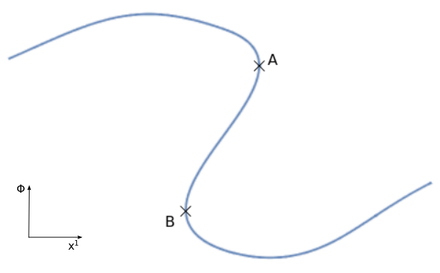
Clearly we have to “choose a branch” of the solution at each point of 2d Minkowsi spacetime. We want to do this so that the solution is as smooth as possible. There are two obvious ways of doing this. We could start from the left of the string and extend until we reach the point of infinite gradient as shown in Fig 1. But beyond this point we have to jump to the other branch, so the solution is discontinuous as shown in Fig. 3. If the discontinuity is approached from the left then the gradient of diverges as we approach . However, if approached from the right the gradient remains bounded up to the discontinuity at . Following out this procedure for the full spacetime produces a globally defined solution of the Born-Infeld theory. After some time, the wavepackets on the Nambu-Goto string separate and the resulting Born-Infeld solution becomes continuous again.
Now note that instead of starting on the left and extending to point we could have started on the right and extended to point . Now the discontinuity would occur at instead of . So now the solution appears as shown in Fig. 3. Approaching the discontinuity from the right, the gradient of diverges at . However approaching from the left, the gradient remains bounded up to the discontinuity at . As above, this procedure gives a globally defined solution of the Born-Infeld theory. This is clearly a different solution from the solution discussed in the previous paragraph.


Starting from initial data prescribed on some line in the far past, the above constructions produce two different solutions which agree with the data on . Now non-uniqueness is to be expected because the solution is singular (at or ), so the corresponding spacetimes will not be globally hyperbolic. Therefore lack of uniqueness is to be expected beyond the Cauchy horizon. However, we will show, in the subluminal case, that the lack of uniqueness occurs before a Cauchy horizon forms. In other words, the two solutions disagree in a region which belongs to for both solutions. This implies that the two solutions cannot arise from the same MGHD of the data on . Therefore MGHDs are not unique.
Clearly there are other ways we could construct Born-Infeld solutions from the Nambu-Goto solution: we do not have to take the discontinuity to occur at either point or at point , we could take it to occur at any point between and . This leads to an infinite set of possible solutions, and an infinite set of distinct MGHDs.
The above discussion was for the subluminal () theory. We will show below that this problem does not occur for the superluminal theory. This is because, in the superluminal theory, from the 2d Born-Infeld perspective, and are timelike separated with (say) occuring to the future of . This implies that lies to the future of the infinite gradient singularity at hence cannot belong to if is a surface to the past of . Therefore there is a unique choice of branch in the superluminal theory. In this theory there is a unique MGHD.
3.5 General solution
The (subluminal) BI scalar theory was solved by Barbashov and Chernikov [5, 6]. We will follow the notation of Whitham [9], who gives a nice summary of their work. Because the superluminal and subluminal theories are related as discussed above, it is easy to write down the general hyperbolic77 7 This solution was obtained using the method of characteristics which only works when the equation is hyperbolic so only hyperbolic solutions are obtained using this method. solution for both cases. Write the Minkowski metric as
| (3.16) |
and define null coordinates
| (3.17) |
The solution is written in terms of a mapping given by
| (3.18) |
where
| (3.19) |
and
| (3.20) |
with and smooth functions such that and decay at infinity fast enough to ensure that the integrals converge.88 8 The latter assumption could be relaxed by replacing the infinite limits of the integrals by finite constants. These two functions can be viewed as specifying the profiles of left moving and right moving wavepackets.
Assuming that is invertible we can write and and the solution is given by
| (3.21) |
Theorem 3.22.
Clearly it will be important to determine whether or not is a diffeomorphism.
Lemma 3.23.
A necessary (although not sufficient) condition for to be a diffeomorphism is that either throughout or throughout .
Proof.
The Jacobian of the map is
| (3.24) |
hence a necessary condition for to define a diffeomorphism is that the RHS cannot vanish at any point of . Since is connected the result follows immediately. ∎
A point on the boundary at which corresponds to a singularity:
Lemma 3.25.
Assume that is a diffeomorphism such that as for some . Let be a smooth curve with as . Then the gradient of the solution at the point diverges as .
Proof.
A calculation gives
| (3.26) |
The result follows immediately. ∎
It can be shown similarly that points of where correspond to a divergence in the second derivative of although we will not need this result below.
We will be mainly interested in causal properties of the metric defined by (3.9). If is a diffeomorphism then we can introduce as coordinates on . The metric defined by (3.9) takes a simple form in these coordinates:
Lemma 3.27.
Note that the vector fields and are null w.r.t. . Let’s determine whether they are future or past directed. Recall (section 2.1) that the time-orientation for is determined by a choice of time orientation for Minkowski spacetime.
Lemma 3.29.
Consider a Born-Infeld solution constructed as in Theorem 3.22. In the subluminal case, is past-directed and is future-directed w.r.t. . In the superluminal case, if then and are both future directed whereas if then they are both past-directed. In either case the spacetime is stably causal.
Proof.
In the subluminal case () we know (section 2.1) that is a global time function for the spacetime so this spacetime is stably causal. From (3.19) and (3.20) one finds and and the result follows.
In the superluminal case (), is timelike w.r.t. so (section 2.1) we choose as a time-orientation on . A calculation gives
| (3.30) |
The inner products (w.r.t. ) of with and can be calculated using (3.28). Clearly these inner products have the opposite sign to and so and are both future directed if this quantity is positive and past directed if it is negative. If then let , which is future-directed and timelike w.r.t. . We then have hence is a global time function for and so is stably causal. Similarly if then is a global time function for . ∎
In the superluminal case, this proves that solutions constructed using Theorem 3.22 cannot exhibit any violation of causality. However, we note that there may be solutions of (3.7) that cannot be obtained using Theorem 3.22. Such solutions would requires multiple charts , each with corresponding coordinates and diffeomorphisms . In any given chart the solution will take the form described above. With multiple charts, it may not be possible to construct a global time function for the superluminal theory.
We are interested in globally hyperbolic developments of initial data. It is very easy to determine whether or not a solution constructed using Theorem 3.22 is globally hyperbolic:
Lemma 3.31.
Consider a Born-Infeld solution constructed as in Theorem 3.22. Then is globally hyperbolic with Cauchy surface if, and only if, is globally hyperbolic with Cauchy surface , where .
Proof.
This is an immediate consequence of (3.28) which shows that and define causally equivalent metrics on . (Here we are not bothering to distinguish the metric on and the metric on defined by pull-back of w.r.t. .) ∎
Thus global hyperbolicity can be checked using the flat metric on . More generally, the causal properties of are the same as those of the flat spacetime .
We will show that, given initial data on a surface , there exist multiple distinct maximal globally hyperbolic developments in the subluminal case () but there is a unique MGHD in the superluminal () case. This difference can be traced to the following property:
Lemma 3.32.
Let be distinct points such that . Then the straight line connecting in the plane is spacelike w.r.t. in the subluminal case and timelike in the superluminal case.
Proof.
Let and have coordinates and respectively. From equations (3.19) and (3.20) we have
| (3.33) |
From the first equation we see that implies and the second equation gives the converse. Hence if, and only if, , i.e., . Since we are assuming we must have and . The first equation then implies that has the same sign as so
| (3.34) |
The result follows from the definition of in Lemma 3.31. ∎
Theorem 3.22 defines a solution in a subset of Minkowski spacetime. The following theorem [6] guarantees a global solution:
Theorem 3.35.
Proof.
Following [6], use (3.20) to write
| (3.36) |
and then substitute into (3.19) to obtain
| (3.37) |
We want to use this equation to determine as a function of . A calculation gives
| (3.38) |
So implies that is a strictly increasing function of and hence there exists at most one solution of (3.37) for any . Given a solution for , (3.36) determines uniquely. This proves that the map is injective.
We now show that there exists exactly one solution of (3.37). Our assumptions on imply that as and as where . Our assumptions on imply that as . So now from (3.38) we see that as . So, at fixed , is strictly increasing and has gradient for . This implies that, at fixed , the map is a bijection from to itself. Hence there exists exactly one solution of (3.37) for given . Hence is a bijection. That is a diffeomorphism now follows from the fact that the RHS of equation (3.24) is everywhere non-zero. ∎
Lemma 3.39.
The solution of Theorem 3.35 is globally hyperbolic.
Proof.
This follows immediately from Lemma 3.31 because so the causal structure w.r.t. is the same as 2d Minkowski spacetime. In the subluminal case, surfaces of constant are Cauchy because is a global time function. In the superluminal case, a surface of constant is Cauchy since the proof of Lemma 3.29 shows that is a global time function. ∎
As discussed above, we need to be a diffeomorphism for equations (3.19), (3.20), (3.21) to define a solution of the Born-Infeld scalar. However, we note that these equations define a solution of the Nambu-Goto string irrespective of whether or not is a diffeomorphism. To see this, take as worldsheet coordinates and replace the LHS of (3.19) and (3.20) by and respectively. Together with this specifies a globally well defined embedding of the string worldsheet into . The worldsheet metric is (3.28). The solution describes a superposition of left moving and right moving wavepackets described by and , each travelling at the speed of light with respect to . The worldsheet metric degenerates at points where . These correspond to “cusp” singularities at which the string worldsheet becomes null. The string is smooth at points where , which correspond to points of infinite gradient like A or B in Fig. 1.
3.6 Example of non-uniqueness in subluminal case
We start by recording that the subluminal Born-Infeld scalar equation of motion (3.7) written out in coordinates reduces to:
| (3.40) |
In this section we will demonstrate the existence of two different maximal globally hyperbolic developments (MGHDs) arising from the same initial data for the above equation. We will do this with an example involving a specific choice of the functions and , and construct solutions using Theorem 3.22.
To construct a solution of (3.40) we choose functions
| (3.41) |
where is a constant. This gives . Hence where . Let . In the plane we have
| (3.42) | ||||
Theorem 3.35 does not apply, and we do not have a global solution. Indeed the map defined by this choice of and is not injective on . In section 3.6.1 we will determine numerically the region in which injectivity fails and explain heuristically how this leads to non-uniqueness of MGHDs. Then, in section 3.6.2 we will use the above example to prove a theorem establishing non-uniqueness of MGHDs.
3.6.1 Numerical demonstration of non-uniqueness of MGHDs
Step 1. We start by showing that, for the example (3.41), is non-injective on but its restriction to a subset of is injective and so we obtain a solution of (3.40) via Theorem 3.22.
The region in which injectivity of fails can be determined numerically99 9 These plots were determined using the FindRoot function in Mathematica to numerically construct an inverse function. A different starting point for the numerics was used for each region. and is shown in Fig. 5: three open regions , and of the plane map to the same region of Minkowski spacetime. Here is the disc . The region is shown in Fig. 5. The inverse image of any point in consists of three points, one in each of , and .1010 10 In the Nambu-Goto string interpretation, is is the region of spacetime in which the string worldsheet folds back on itself as in Fig. 1. However, the map is injective on and (3.42) implies that the condition of Lemma 3.23 is satisfied on so defines a diffeomorphism from to . Hence Theorem 3.22 defines a solution of (3.40).


Step 2. Next we will show that the solution is not a GHD but, by restricting its domain, we can construct a GHD.
Lemma 3.31 establishes that is globally hyperbolic if, and only if, is globally hyperbolic. Introduce coordinates in the plane such that
| (3.43) |
In these coordinates we have
| (3.44) |
and Lemma 3.29 implies that is future-directed. The causal properties of (and hence ) in the plane are easy to read off from Fig. 5. In particular it is clear that the region is not globally hyperbolic w.r.t. so is not globally hyperbolic w.r.t. . Consider an initial surface defined by , as shown in Fig. 5. Let be the domain of dependence of in . Then by restricting to we obtain a GHD of the initial data on . Appealing to Lemma 3.31, where is the domain of dependence of in . Viewed as a subset of , is bounded by the future Cauchy horizon shown in Fig. 5, which maps to a corresponding future Cauchy horizon in Fig. 5.
Step 3. Now we will show that the GHD is not maximal and it can be smoothly extended to give a GHD that contains part of region . We will show that this extended GHD is smooth on the “left” boundary of but singular on the “right” boundary of .
We enlarge the GHD by pushing the left large dashed orange line of Fig. 5 into region until it is tangent to the boundary of . Specifically, consider the region defined in Fig. 7. Since contains no points of or , the map is still injective on this enlarged region and still satisfies (3.24), hence is a diffeomorphism and so Theorem 3.22 defines a solution where . Furthermore, is globally hyperbolic with Cauchy surface and so is globally hyperbolic with Cauchy surface . Hence is a GHD of the initial data on . The region is shown in Fig. 7: it extends across the left boundary of all the way to the right boundary of . This right boundary is not part of , indeed the solution is discontinuous across this boundary.1111 11 In the Nambu-Goto string interpretation, the string worldsheet on a surface of constant intersecting resembles Fig. 3 with point on the right boundary of .
Consider a curve approaching the right boundary of from the left (i.e. from within ) as in Fig. 7. Then is a curve approaching the solid red curve of Fig. 7 from within . Since on this red curve, Lemma 3.25 implies that the gradient of diverges along as one approaches the boundary. Thus the gradient of diverges along the right boundary of when approached from the left. On the other hand, if is a curve approaching this boundary from the right (i.e. from outside ) as in Fig. 7 then approaches the dotted red curve of Fig. 7, which is in the region where so the gradient of remains bounded along . Hence the gradient of is bounded as one approaches the right boundary of from outside .


Step 4. Finally we show that there is a different way of extending to give a GHD and that this implies non-uniqueness of MGHDs.
We construct this new extension of as follows. Define to be the reflection of under . So is an extension of into region . Everything we’ve said about is true also of and so this defines another GHD where . In this case, extends across the right boundary of all the way the the left boundary of , where the gradient of diverges when approaching from the right.1212 12 In the Nambu-Goto string interpretation, this corresponds to Fig. 3 with point on the left boundary of .
We now have two different GHDs of the same intial data on , and . These two solutions agree in but they differ in because has divergent gradient on the right boundary of whereas has divergent gradient on the left boundary of . Thus the corresponding maximal GHDs must differ in . This demonstrates the non-uniqueness of maximal GHDs for (3.40).
We will now discuss this result and highlight properties of our example that are relevant to the general results of Section 4.
Consider the intersection shown in Fig. 8. Note that this is disconnected, consisting of two connected components. One component contains but no points of and the other component is a subset of . The two solutions agree on the former component but they disagree on the latter component. In Section 4 we will prove that this disconnectedness is a necessary condition for two GHDs to differ in some region.

Another point to emphasize is that the boundary of consists of a section (along the right boundary of , between the lower black dot and the orange curves of Fig. 7), which can be approached from both sides (either the left or the right) within . In other words lies on both sides of its boundary. (The same is true for .) In section 4 we will show that this property is a necessary condition for non-uniqueness of MGHDs.
We have shown that there exist two distinct MGHDs arising from the same data on . In fact one can show that there are infinitely many such MGHDs (cf section 3.4). The different MGHDs all agree in the region but they differ in . In section 4 we will define the maximal unique globally hyperbolic development (MUGHD) of the initial data on as follows. is the largest open subset of Minkowski spacetime on which the solution is uniquely determined by the data on . Such a development is necessarily globally hyperbolic with Cauchy surface . For the above example, we have and . As we have seen, the solution can be extended, whilst maintaining global hyperbolicity, but not in a unique way. From Figs 5 and 5 we see that the future boundary of consists of a singular point (the lower black dot in Fig. 5) from which emanate a pair of spacelike (w.r.t. ) curves which connect to a pair of null (w.r.t. ) curves. The solution can be smoothly, but not uniquely, extended across these spacelike and null curves.
The extendibility across the spacelike curves is a new kind of breakdown of predictability. Fig. 5 suggests that we should view these spacelike curves (the early time sections of the red and blue dotted curves) as a “consequence” of the formation of a singularity (the black dot). This interpretation is suggested if one uses as a time function (e.g. in a numerical simulation). However, since these curves are spacelike, they are not in causal contact with the singularity. Furthermore, it is just as legitimate to use as a time function. From this point of view, Fig. 5 shows that the spacelike curves form before (i.e. at earlier ) the singular point. So it is incorrect to ascribe the breakdown of predictability to the formation of the singularity.
This behaviour is worrying. Given a development of the data on , there is no general way of determining, from the solution itself, which region of it belongs to the MUGHD. To determine this region one has to construct all GHDs with the same initial data! This is much worse than the failure of predictability associated with the formation of a Cauchy horizon because the location of a Cauchy horizon within a development can be determined from the solution itself.
How would the non-uniqueness of MGHDs manifest itself in, say, a numerical simulation? The answer is that the solution will depend not just on the initial data but also on the choice of time function. To see this, consider the globally hyperbolic development . Since is a Cauchy surface we can choose a global time function for such that is a surface of constant time. We can do the same for . Of course these two time functions are different but either could be used for a numerical evolution starting from the data on . For points in the MUGHD , the results of these two numerical evolutions will agree. However, for points in , the results will disagree. In practice one would not know a priori which points belong to the MUGHD, i.e., one would not know in what region the results of the numerical evolution are independent of the choice of time function.1313 13 Since we are dealing with a subluminal theory, one could just declare that is a preferred time function and ignore the above problems. However this is unsatisfactory: if one uses as the time function (with a surface of constant at sufficiently early time) then from Fig. 5 the evolution must stop at the line of constant passing through the singularity corresponding to the (lower) black dot so one obtains only part of the MUGHD.
Note that, for any solution, the domain of dependence of defined using the Minkowski metric is a subset of the domain of dependence of defined using . Hence a solution which is globally hyperbolic w.r.t. is also globally hyperbolic w.r.t. . We could therefore ask about uniqueness of MGHDs defined w.r.t. instead of w.r.t. . We’ll refer to these as -MGHDs. For the above example, there is indeed a unique -MGHD: it is bounded to the future by two future-directed null (w.r.t. ) lines emanating from the lower black dot in Fig. 5. We’ll prove in Section 4 that any subluminal equation always admits a unique -MGHD, which is a subset of the MUGHD. However, if the speed of propagation w.r.t. is much less than the speed of propagation w.r.t. then the -MGHD will not be a very useful concept because it will not contain a large part of the MUGHD.
We have used the Born-Infeld scalar as an example exhibiting non-uniqueness of MGHDs. This example is rather artificial because there is a “more fundamental” underlying theory, namely the Nambu-Goto string, for which there is no problem with predictability. However, our point is that if this pathological feature can occur for a particular scalar field theory then it is to be expected to occur also for other scalar field theories for which there is no analogue of the Nambu-Goto string interpretation.
This ends the heuristic discussion of our example of non-uniqueness. We will now present a rigorous proof of the non-uniqueness of MGHDs.1414 14 Note that the regions , etc in the proof of this theorem are defined slightly differently from the regions defined in the discusion above.
3.6.2 Theorem on non-uniqueness of MGHDs
Theorem 3.45.
For the equation (3.40) there exist two GHDs and of the same initial data posed on such that there exists an with .
Proof.
We begin by remarking that we will prove the statement of the theorem with the hypersurface replaced by for . This represents no loss of generality since the equation (3.40) is invariant under translations in . We will construct the two GHDs using Theorem 3.22 and Lemma 3.31.
We choose and as in (3.41) and recall equation (3.42). We start by investigating the map defined by (3.19) and (3.20).
Step 1: Analysis of the level sets of .
We begin by noticing that the function
| (3.46) |
clearly satisfies for all , and thus its level sets are closed, embedded, one-dimensional submanifolds which foliate . The leaf can be written as a graph over the -axis: . It follows from , that the graph is strictly monotonically increasing. Moreover, we have for and for , where .
Next we investigate the qualitative behaviour of the intersection of the leaves of constant with the circle of radius . Let denote the restriction of to the circle of radius . Since the latter is compact, it follows that takes on its minimum and its maximum . Hence, the differential of must have at least two zeros.
We now parametrise the circle of radius by where , and we compute . It follows that
| (3.47) |
Let us first consider the upper arc of the circle, i.e., and the minus sign in (3.47). We try to solve
| (3.48) |
Clearly, this does not have any solution for . We also remark that regularising for by multiplying it, and thus also (3.48), by , shows that cannot be an extremum of . It follows that does not have any extrema in the quadrant .
On the other hand we have
and
It follows that can have at most one extremum in the quadrant .
Similarly, by considering the lower arc of the circle and the plus sign in (3.47) we find that does not have any extrema in the quadrant and at most one extremum in the quadrant . It thus follows that has exactly two extrema, one in the quadrant and one in the quadrant . Moreover, it is easy to see that the extremum in the quadrant is the global maximum (for example this follows from ) and the extremum in the quadrant is the global minimum. Furthermore it follows that is strictly monotonically increasing along the two segments of the circle of radius that connect the minimum of with its maximum. In particular, takes on every value exactly twice.
In conclusion, we have established the following qualitative picture: The curves of constant for are disjoint of the circle of radius and lie below it, the curve touches the circle in exactly one point in the quadrant , the curves of constant for intersect the circle in exactly two points, the curve touches the circle in exactly one point in the quadrant , and finally the curves of constant for are disjoint of the circle of radius and are lying above it. This behaviour is summarised in Figure 9.

If is a diffeomorphism, then Theorem 3.22 gives a solution of (3.40). By (3.24) and (3.42) is a local diffeomorphism everywhere away from the circle .
Step 2: We analyse in which regions in the map is injective.
For this, let us assume that for we have
| (3.49) |
Obviously this entails that and both have to lie on the same curve . Recall from (3.37) that along the curve , the value of the coordinate is a function of : . Also recall from (3.38) that we have
| (3.50) |
It now follows from our qualitative understanding of the curves of constant together with (3.42) that for or we have for all . Thus, for such , is a strictly monotonically increasing function in along and thus (3.49) implies . It is easy to see that is still strictly monotonically increasing along , since those curves touch only in one point and thus the right hand side of (3.50) only vanishes at one point. Thus, we have shown
| is injective in the regions and . | (3.51) |
However, for the right hand side of (3.50) is negative inside the circle of radius . Let be the value of at which enters the circle of radius and the value at which leaves the circle of radius . Thus, the function is strictly monotonically decreasing for . For the right hand side of (3.50) is positive and thus is strictly monotonically increasing for such . Moreover, it follows from (see (3.41) and below) that for , the right hand side of (3.50) tends to . Thus we have for and for . The qualitative behaviour of the function , which we have just established, is depicted in Figure 10.

Hence, is a local maximum and is a local minimum of . For each there exist, by the intermediate value theorem and the monotonicity properties, exactly three points with , . Setting , this determines three distinct points , , which are all mapped to under . (Two of these points lie outside the circle and one lies inside.) Hence, we have shown that is not injective in .
To understand the subsets of on which is injective, let us first observe that the set has two connected components. We denote the ‘left’ component1515 15 I.e., the component which contains points of arbitrarily large and negative -coordinate. by and the ‘right’ component by . It follows directly from (3.42) and (3.50) that
| is injective on as well as on . | (3.52) |
Moreover, we note that inside the circle of radius the right hand side of (3.50) is bounded from below by . Thus, for the function can decrease in between and by at most . On the other hand, since , the right hand side of (3.50) is bounded from below by a positive constant in . It thus follows that we can choose large enough such that for all . Since we have for all this shows
Hence, we have shown
| (3.53) |
Step 3: Construction of the two solutions and .
Let now denote the point of contact of with the circle . We have and . We now define the region
| (3.54) |
cf. Figure 12. It follows from (3.51) and (3.53) that is injective on and thus a diffeomorphism onto its image. Recall that we have
Thus the hypersurface is given in the plane by
It follows from the trivial bounds on the integrals that for the hypersurface is contained in .1616 16 The reason for including in (3.54) was exactly to ensure this. We now define our first GHD by setting and defining by Theorem 3.22. It is easy to convince oneself, using Lemma 3.31, that the domain is indeed globally hyperbolic with Cauchy hypersurface .
To define the second GHD , we set
See also Figure 12. It follows from (3.51) and (3.52) that is injective on and thus we can set and define by Theorem 3.22. Again, it is easy to convince oneself that the domain is indeed globally hyperbolic with Cauchy hypersurface .


Step 4: We show that there is an with .
For this consider a curve . By continuity we can choose small enough such that the curve intersects the circle of radius at and such that and . Since , the qualitative analysis of below (3.51) applies which was summarised in Figure 10. It follows that there exist and and a strictly monotonically increasing function
and a second strictly monotonically increasing function
such that
holds for all . See also Figure 13 and the discussion following (3.51).

We remark the following:
Remark 3.55.
We emphasise that the two GHDs constructed in the proof of Theorem 3.45 are smooth. Hence, the non-uniqueness mechanism exhibited does not stem from a loss of regularity of the solution.
Remark 3.56.
We note that the two GHDs constructed in the proof of Theorem 3.45 are not maximal. However, an application of Zorn’s Lemma (!) to the set of globally hyperbolic extensions of shows that there exists a MGHD which contains . In the same way one shows the existence of a MGHD which contains . These two MGHDs are clearly distinct. In fact one can even show that there are infinitely many distinct MGHDs of the constructed initial data. We leave the details to the reader.
Remark 3.57.
The initial data constructed in the proof of Theorem 3.45 are not compactly supported. However, by a standard domain of dependence argument one can cut off the initial data outside a large enough ball to produce compactly supported initial data and two GHDs thereof which satisfy the statement of Theorem 3.45.
The following remark might be skipped and come back to when referred to later in Section 4.
Remark 3.58.
Recall that equation (3.40) (which is (3.7) multiplied by ) is not manifestly hyperbolic, i.e., a quasilinear wave equation of the form (4.61) which we will consider in Section 4. Its principal symbol is
and the determinant is . It follows from (3.26) and (3.41) that for the two hyperbolic solutions constructed above we have
We can thus modify the principal symbol of (3.40) in the region to make it Lorentz-metric valued for all (and keeping it subluminal), thus creating a subluminal quasilinear wave equation (i.e. a quasilinear equation for which every solution is hyperbolic) which is still solved by our two GHDs of the same initial data constructed above which take different values at a point that lies in both of their domains.
3.7 Uniqueness for superluminal case
Non-uniqueness of MGHDs is not a problem in the superluminal () case. We will prove this for an arbitrary superluminal equation in section 4 below. In this section we will discuss briefly the interpretation of the example (3.41) in the superluminal case.
In the superluminal case, recall that the Minkowski metric (3.16) is
| (3.59) |
and we choose time orientation . Defining coordinates in the plane as in (3.43) gives, for the flat metric of Lemma 3.31
| (3.60) |
Now consider the example (3.41). We want to construct a solution using Theorem 3.22 so assume that is a diffeomorphism. Lemma 3.23 implies that either or lies outside . We consider the latter case, so in . The proof of Lemma 3.29 reveals that is a global time function for (or ) so we take our initial surface where is a line where is large enough so that lies to the past of as shown in Fig. 15.1717 17 Equivalently we could define to be a surface where is chosen large enough to make spacelike w.r.t. . However, this would gives plots with a lot of white space between (or ) and the region of interest.


The unique MGHD is obtained by taking to be the region defined in Fig. 15. The future boundary of is the union of a spacelike curve (a segment of the boundary of ) along which the gradient of diverges (by Lemma 3.25), and a pair of null curves across which the solution is smoothly extendible (but not as a GHD).1818 18 Note that the extendibility across the null sections of the boundary implies that the analogue of the strong cosmic censorship conjecture is false for the superluminal equation. But the behaviour is much better than in the subluminal case for which the object one needs to define to formulate this conjecture (the MGHD) is not even unique! The corresponding picture in Minkowski spacetime is shown in Fig. 15.
The reason that there is a unique MGHD in the superluminal case but not in the subluminal case was identified in Lemma 3.32. In the subluminal case, different GHDs can be constructed by including points from or from , or from both. But in the superluminal case, Lemma 3.32 implies that lies to the future of so from any point of there is a past directed timelike curve that ends on the boundary of and hence does not cross . So no point of can belong to the domain of dependence of .
3.8 Higher dimensions
It is easy to see that the pathological behaviour in the subluminal case is not restricted to two spacetime dimensions. The Born-Infeld scalar field theory in -dimensional Minkowski spacetime is defined by generalizing the action (3.6) to dimensions. The two dimensional theory can be obtained trivially from the dimensional theory by assuming that does not depend on of the spatial coordinates. Hence our 2d solutions can be interpreted as solutions in dimensions with translational invariance in directions. Such solutions do not decay at infinity. However, given initial data for such a solution, one could modify the data outside a ball of radius so that it becomes compactly supported. In the subluminal case, the resulting solution would be unchanged in the region inside the ingoing Minkowski lightcone emanating from the surface of this ball. Hence if is chosen large enough then the evolution of the solution inside the ball will behave as discussed above for long enough to see non-uniqueness of MGHDs.
In the higher-dimensional superluminal case, there is a unique MGHD: we will prove below that any superluminal equation always admits a unique MGHD.
4 Uniqueness properties of the initial value problem for quasilinear wave equations
4.1 Introduction
In this section we consider a quasilinear wave equation of the form
| (4.61) |
where , is a smooth Lorentz metric valued function,1919 19 All the results presented in this section generalise literally unchanged to the setting of Section 2, where one does not assume that in (4.61) is a Lorentz metric valued function, but one restricts consideration to hyperbolic solutions, i.e., solutions of (4.61) for which is Lorentz metric valued. The only slight modification necessary is for the proof of the local existence result, Theorem 4.75. Here one can for example cut off the principal symbol of the quasilinear equation in the fashion of Remark 3.58 to create a quasilinear wave equation and then apply the local existence result for quasilinear wave equations to show local existence of hyperbolic solutions for quasilinear equations with hyperbolic initial data. is smooth with , and the coordinates used for defining (4.61) are the canonical coordinates on .
Let be a connected hypersurface of . Initial data for (4.61) on consists of a smooth real valued function and a smooth one form (with values in ) along such that holds for all vectors tangent to and such that the hypersurface is spacelike with respect to the Lorentzian metric . A globally hyperbolic development (GHD) of initial data on a hypersurface for (4.61) consists of a smooth solution of (4.61) ( being open) with and , , and such that is globally hyperbolic with respect to the Lorentzian metric with Cauchy hypersurface .
As we will show/recall in the following, the initial value problem for the equation (4.61) with initial data given on a hypersurface is locally well-posed. Here, we mean by this that the following two properties hold:
- 1.
there exists a globally hyperbolic development of the initial data
- 2.
given two globally hyperbolic developments and of the same initial data, then there exists a common globally hyperbolic development (CGHD), that is, a globally hyperbolic development of the initial data with and .
Note that the second property is only a weak version of what one might understand under ‘local uniqueness’, since it allows for the existence of a third globally hyperbolic development of the same initial data such that there exists an with .2020 20 We will discuss how this might happen at the end of Section 4.7.
The aim of this section of the paper is to investigate the uniqueness properties for solutions of quasilinear wave equations. In Section 4.2 we first prove the second property of the local well-posedness statement from above and then establish the main theorem of this section: two globally hyperbolic developments of the same initial data agree on the intersection of their domains if this intersection is connected. Section 4.3 then specialises to quasilinear wave equations (4.61) with the property that
| there exists a vector field on such that is timelike with respect to for all . | (4.62) |
In particular superluminal equations have this property. We show that for such equations the intersection of the domains of two globally hyperbolic developments of the same initial data is always connected – and we thus obtain that any two globally hyperbolic developments agree on the intersection of their domains. The case of subluminal equations is considered in Section 4.4. Here, we show that if one of the two globally hyperbolic developments is also globally hyperbolic with respect to the Minkowski metric, then again, the intersection of the domains is connected – and we can thus apply our main theorem from Section 4.2.
The next three sections deal with existence questions: Section 4.5 proves the first property of the above local well-posedness statement, Section 4.6 establishes the existence of a unique maximal globally hyperbolic development for quasilinear wave equations with the property (4.62), and Section 4.7 considers subluminal equations and shows the existence of a maximal region on which solutions are unique and which is globally hyperbolic (i.e. a MUGHD).
The final section, Section 4.8, present a uniqueness criterion for general quasilinear wave equations of a very different flavour. It states that if there exists a maximal globally hyperbolic development with the property that its domain of definition always lies to just one side of its boundary, then this maximal globally hyperbolic development is the unique one. In particular this implies uniqueness of the MGHD constructed in Ref. [7].
4.2 Uniqueness results for general quasilinear wave equations
Proposition 4.63 (Local uniqueness).
Let and be two globally hyperbolic developments for (4.61) of the same initial data prescribed on a hypersurface . Then there exists a common globally hyperbolic development .
Proof.
For let be an open neighbourhood of on which there exists slice coordinates for and in which the Lorentzian metric given by the initial data is -close to the Minkowski metric. Moreover, we require . Let be an open neighbourhood of in the closure of which is compactly contained in . The standard literature methods (see for example [17]) ensure that there is an open neighbourhood of with the property that any two solutions, which are defined on and attain the given initial data on , agree, and such that is globally hyperbolic with Cauchy hypersurface . It thus follows that . We now set . It is immediate that and agree on this set and that is globally hyperbolic with Cauchy hypersurface . ∎
One can now ask whether global uniqueness holds, which is the property that if and are two globally hyperbolic developments of the same initial data, then and agree on . Note that ‘global’ refers to the property that ‘the two solutions agree in all of ’ – in contrast to the local result provided by Proposition 4.63, which only guarantees uniqueness in some smaller subset of .
The last author sketched an idea for a proof of global uniqueness in Section 1.4.1 of [13]. However, this sketch has the flaw that it tacitly assumes that given two globally hyperbolic developments and of the same initial data, that is then connected – which is in general not true as illustrated by the example presented in Section 3.6 of this paper, see in particular Remark 3.58. The necessity of the assumption of connectedness enters in the sketch as follows: One starts by considering the maximal globally hyperbolic region contained in on which and agree (i.e. the maximal common globally hyperbolic development (MCGHD)) and one would like to show that this region coincides with . Assuming one can find a boundary point of in provided is connected. The argument then proceeds by constructing a spacelike slice through a suitable boundary point and appealing to the local uniqueness result in order to conclude that and also agree on a neighbourhood of this slice and thus on an even bigger globally hyperbolic region than – a contradiction to the maximality of . This is roughly how one proves global uniqueness under the condition that is connected. Note that if is disconnected, the same argument shows that the domain of the MCGHD equals the connected component of that contains .
For the Einstein equations one does not need to condition the global uniqueness statement, since one has the freedom to construct the underlying manifold – there is no fixed background. We will explain this in the following: Given two globally hyperbolic developments and for the Einstein equations one constructs a bigger one in which both are contained (and thus proves global uniqueness) by glueing and together along the MCGHD of and . However, in the case that and are two globally hyperbolic developments of a quasilinear wave equation on a fixed background such that is disconnected, glueing them together along the MCGHD (which equals the connected component of which contains the initial data hypersurface), would yield a solution which is no longer defined on a subset of , but instead on a manifold which projects down on and contains the other connected components of twice. Of course this is not allowed if we insist that solutions of (4.61) should be defined on a subset of . So the key difference between the Einstein equations and a quasilinear wave equation (4.61) is that for the former the underlying manifold is constructed along with the solution whereas for the latter, it is fixed a priori. This is the reason why one does not need to condition the global uniqueness statement for the Einstein equations.
Theorem 4.64.
Let and be two globally hyperbolic developments of (4.61) arising from the same initial data given on a connected hypersurface . Assume that is connected. Then and agree on .
Proof.
Step 1: We construct the maximal common globally hyperbolic development of and .
Given two globally hyperbolic developments and of (4.61) arising from the same initial data on , we consider the set of all common globally hyperbolic developments. By Proposition 4.63 we know that this set is non-empty. We define , where and for . It is immediate that this is well-defined and that is a common globally hyperbolic development with the property that any other common globally hyperbolic development is a subset of . We call the maximal common globally hyperbolic development.
We now set out to show that , from which the theorem follows. Assume that . Since we assume that is connected, there exists then a point .2121 21 denotes the boundary of in . Without loss of generality we assume that .2222 22 The notation denotes the causal future of in with respect to the Lorentzian metric . The notations for the causal past , and timelike future/past are analogous. We refer the reader to [16] for the basic notions of causality theory.
Step 2: We show in the following that there exists a point such that
| (4.65) |
holds. Such a point can be thought of as a point where the boundary is spacelike.
In the following the causality relations are with respect to the metric . Let be as above. If (4.65) holds for , we are done – hence, we assume that there is a second point . The global hyperbolicity of with Cauchy hypersurface together with the openness of the timelike relation implies that is achronal. Hence, the past directed causal curve with and is a null geodesic. Using the global hyperbolicity of it follows that , since if there were a with , then we would also obtain – and if , then by the openness of the timelike relation one could find a past directed timelike curve starting from a point in close to that lies completely in and ends at a point in close to . Moreover, , since and by the smoothness of , is also a past directed null geodesic in the globally hyperbolic – hence, it cannot leave without first crossing .
We now extend maximally in to the past. The global hyperbolicity of entails that has to intersect , thus entering and leaving . We now consider . The argument from the last paragraph shows that this is a connected interval, and the closedness of in together with implies that for some . Note also that it follows from the last paragraph that . We claim that satisfies (4.65).
Assume does not satisfy (4.65). Then there is a point . As before, one can connect and by a past directed null geodesic that is contained in . However, by the definition of , this null geodesic cannot be the continuation of . We can thus connect and by a broken null geodesic, and thus by a timelike curve in – contradicting the achronality of .
Step 3: Let be as in (4.65). We claim that for every open neighbourhood of there exists a point such that holds.
To show this, let be as above and assume the claim was not true. Then there exists a neighbourhood of such that for all there exists a point . In particular, let us choose a sequence and with for all and . By the global hyperbolicity of we know that is compact, and thus, so is . Hence, we can assume without loss of generality that . Since the causality relation is closed on globally hyperbolic Lorentzian manifolds, we obtain . Moreover, since , we clearly have . By (4.65) we cannot have , thus we have . This, however, contradicts the global hyperbolicity of , since, by the openness of the timelike connectedness relation , we can find a past directed timelike curve starting at a point contained in close to and ending at a point in without crossing the Cauchy hypersurface .
Step 4: We construct a spacelike hypersurface that contains at least one point of .
Let be as in (4.65) and consider a convex neighbourhood of . By the previous step we can find a point such that holds. We denote by the (past) time separation from in , i.e., for in we have
where denotes the Lorentzian length of . If , then we set . It follows from [16, Chapter 5, 34. Proposition] that restricted to is given by
hence, is smooth on and continuous on . Since is compactly contained in , there exists an with
| (4.66) |
Clearly, we have . We set . It follows from [16, Chapter 5, 3. Corollary] that is a smooth spacelike hypersurface. Moreover, we have , since if we had , we could extend the unique timelike geodesic from to slightly such that it still remains in , contradicting (4.66). Hence, contains at least one point of . Since we have chosen to be contained in the future of in , we in particular have . Thus, the same argument as before shows .
Step 5: Since and agree on , by continuity they (and their derivatives) also agree on . Consider now a point in and take a simply connected neighbourhood thereof such that is a closed hypersurface in . By [16, Chapter 14, 46. Corollary], is acausal in .
Let denote the domain of dependence of in and the domain of dependence of in . and are both globally hyperbolic developments of the same initial data on , and thus by Proposition 4.63 they agree in some small globally hyperbolic neighbourhood of . Note that contains at least one point of . Moreover, it is easy to see that is globally hyperbolic with Cauchy hypersurface : an inextendible causal curve in has to intersect and thus, to the past, enter , where the last inclusion follows from and the global hyperbolicity of . This, however, contradicts the maximality of . ∎
Remark 4.67.
Let us remark that the proof in particular shows that under the assumptions of Theorem 4.64 the intersection is the maximal common globally hyperbolic development of and . If we fix a choice of normal of the initial data hypersurface and stipulate that it is future directed in as well as in , then it follows in particular that a point , which lies to the future of in , also lies to the future of in . Similarly for the past.
The following is an immediate consequence of the previous theorem. It shows that global uniqueness can only be violated for quasilinear wave equations in a specific way.
Corollary 4.68.
Let and be two globally hyperbolic developments of (4.61) arising from the same initial data on a connected hypersurface . If there exists an with , then is not connected.
In particular, we recover that globally defined solutions are unique:
Corollary 4.69.
In the next two sections we consider two globally hyperbolic developments and of the same initial data and discuss criteria that ensure that is connected. Here, the choice of the initial data hypersurface plays an important role. This can already be seen from the special case of the linear wave equation in Minkowski space: consider a spacelike but not achronal hypersurface that winds up around the -axis in . Prescribing generic initial data on this hypersurface, the extent of the future development restricts the extent of the past development. Given two globally hyperbolic developments, their intersection is in general not connected and global uniqueness does not hold. However, it is easy to show (see also Section 4.3) that for spacelike initial data hypersurfaces which are moreover achronal, this pathology for the linear wave equation in Minkowski space cannot occur. This example shows that any result demonstrating connectedness of for more general quasilinear equations will require some additional assumptions on the initial surface analogous to the achronality assumption in Minkowski spacetime.
4.3 Uniqueness results for superluminal quasilinear wave equations
In the following we consider quasilinear wave equations (4.61) that enjoy property (4.62), i.e., that there exists a vector field on such that is timelike with respect to for all . In particular, superluminal equations enjoy this property, since one can take where are inertial frame coordinates. We will show that for such equations the complication of being disconnected cannot arise, as long as the initial data is prescribed on a hypersurface with the property that every maximal integral curve of intersects at most once.2323 23 For a superluminal equation with , any which is a Cauchy surface for Minkowski spacetime has this property. Of course also has to obey the assumptions discussed at the beginning of section 4.1 e.g. has to be spacelike w.r.t. .
Lemma 4.70.
Assume that there exists a vector field on such that is timelike with respect to for all , where is as in (4.61). Let and be two globally hyperbolic developments of (4.61) arising from the same initial data on a connected hypersurface which has the property that every maximal integral curve of intersects at most once. Then is connected.
Proof.
Let , be two globally hyperbolic developments arising from the same initial data on and let . Let be the maximal integral curve of through . By assumption, intersects at most once. Since and are timelike curves in , , respectively, and , are globally hyperbolic with Cauchy hypersurface , it follows that intersects exactly once and that the portion of from to is contained in as well as in . This shows the connectedness of .
∎
Let us remark, that one can replace in the above lemma the assumption that is a connected hypersurface such that every maximal integral curve of intersects at most once, with the assumption that is a hypersurface that separates into two components. We leave the small modification of the proof to the interested reader.
Corollary 4.71.
Assume that there exists a vector field on such that is timelike with respect to for all , where is as in (4.61) and that initial data is posed on a connected hypersurface which has the property that every maximal integral curve of intersects at most once.
Given two globally hyperbolic developments and , we then have for all .
4.4 Uniqueness results for subluminal quasilinear wave equations
We recall that a quasilinear wave equation of the form (4.61) is called subluminal iff the causal cone of is contained inside the causal cone of the Minkowski metric . As shown in Section 3.6 of this paper, and in particular see Remark 3.58, in general global uniqueness does not hold for subluminal quasilinear wave equations – even if the initial data is posed on the well-behaved hypersurface . However, as we shall show below, developments are unique in regions that are globally hyperbolic with respect to the Minkowski metric. Recall the terminology introduced in Section 3.6: we say that a GHD of a subluminal quasilinear wave equation is a -GHD iff it is also globally hyperbolic with respect to the Minkowski metric with Cauchy hypersurface . As usual, denotes here the initial data hypersurface.
Lemma 4.72.
Let and be two GHDs of a subluminal quasilinear wave equation (4.61) arising from the same initial data given on a connected hypersurface that is achronal with respect to the Minkowski metric . Assume, moreover, that is a -GHD. Then is connected.
Proof.
Let and assume without loss of generality that . We claim that this implies . To see this, assume . Hence, there exists a future directed timelike curve from to in and a future directed timelike curve from to in . They are both future directed timelike with respect to the Minkowski metric. Concatenating the two curves gives a contradiction to the achronality of with respect to . This shows .
Let be a curve in that starts at and is timelike, past directed, and past inextendible w.r.t. . It thus intersects . However, is also a past directed timelike curve with respect to , and the global hyperbolicity of with respect to implies that cannot leave without first intersecting . Thus, the segment of from to is contained in . This shows the connectedness of . ∎
Together with Theorem 4.64 the above lemma yields
Corollary 4.73.
Let and be two GHDs of a subluminal quasilinear wave equation (4.61) arising from the same initial data given on a connected hypersurface that is achronal with respect to the Minkowski metric . Assume, moreover, that is a -GHD. Then on .
Remark 4.74.
Let us remark that better bounds on the light cones of translate into an improvement of the uniqueness results. Above, we have only made use of the trivial Minkowski bound on the light cones for subluminal equations. If, for example, for a specific subluminal equation one can improve the a priori bound on the light cones of for certain initial data, then one can also improve the uniqueness result for these initial data.
4.5 Local existence for general quasilinear wave equations
This section provides the other half of the local well-posedness statement for quasilinear wave equations with data on general hypersurfaces: the local existence result.
Theorem 4.75 (Local existence).
Given initial data for a quasilinear wave equation (4.61), there exists a globally hyperbolic development.
Moreover, this result is needed for the existence results of a unique maximal GHD for superluminal quasilinear wave equations and of a maximal unique GHD for subluminal quasilinear wave equations.
Note that Theorem 4.75 with data on the hypersurface is a standard literature result. We prove Theorem 4.75 by using the standard literature result to construct solutions in local coordinate neighbourhoods around points of the general initial data hypersurface and then patching them together. Note that this has to be carried out carefully to ensure that different local solutions agree on the intersection of their domains. Here we make use of Theorem 4.64 to guarantee uniqueness if the intersection of their domains is connected.
Proof.
Given the initial data on the hypersurface (as discussed in Section 4.1) we choose a timelike normal along and extend it smoothly off to yield a vector field which we also denote with . There exists an open neighbourhood of in and an open neighbourhood of such that the flow of is a diffeomorphism from onto . For let be an open neighbourhood of on which there exists slice coordinates in which the Lorentzian metric determined by the initial data is -close to the Minkowski metric. Let be a neighbourhood of in with closure that is compactly contained in . The standard energy methods in the literature (see for example [17]) yield that there exists a globally hyperbolic development for (4.61) of the initial data on , where . Moreover, by choosing smaller if necessary, we can assume that is timelike on . We now claim that for all we have on .
To show this, assume that and let be a connected component of . Consider an . The integral curve of through is a timelike curve in as well as in , and thus it has to intersect and, moreover, its segment from to is contained in . This shows that is non-empty. It will follow a posteriori that is connected, but for the time being let be a connected component of . We denote with the domain of dependence of in with respect to the Lorentzian metric arising from and , respectively. Since by the above argument involving the timelike integral curves of , the intersection is connected, Theorem 4.64 implies that we have on .
Assume now that . Since is connected, there exists an . Without loss of generality we assume that lies to the future of . Let be any past directed and past inextendible causal curve in with respect to the metric arising from that starts at . The global hyperbolicity of (see Remark 4.67) implies
| (4.76) |
and hence the part of to the causal future of is also a past directed causal curve in with respect to . The global hyperbolicity of and shows that has to intersect , and by (4.76), in fact intersects . This, however, gives the contradiction by definition of the domain of dependence. We thus conclude that . Moreover, it now follows that holds on . Hence, we can finish the proof by constructing a GHD of the given initial data on by setting and for . ∎
4.6 The existence of a unique maximal GHD for superluminal quasilinear wave equations
Theorem 4.77.
Assume that there exists a vector field on such that is timelike with respect to for all , where is as in (4.61) and that initial data is posed on a connected hypersurface which has the property that every maximal integral curve of intersects at most once.
Given such initial data, there then exists a unique maximal globally hyperbolic development , that is, a globally hyperbolic development with the property that for any other globally hyperbolic development of the same initial data we have and .
Proof.
We consider the set of all globally hyperbolic developments arising from the given initial data on as above. Note that this is a set and, moreover, it is non-empty by Theorem 4.75. We now define and by for with . Note that the latter is well-defined by Corollary 4.71. In order to see that is a globally hyperbolic development of (4.61) arising from the given initial data, consider an inextendible timelike curve , where , and let . We have for some . Let be the maximal interval containing such that maps into . Since is an inextendible timelike curve in , there exists a with . Thus, it remains to show that does not intersect more than once. Without loss of generality we assume that is future directed in . We consider
We already know that is non-empty. Moreover, is clearly open, since each is open. Let be a sequence with as , and let be such that . By the openness of there is with . Since , there exists with . It now follows from Remark 4.67 that must also lie to the future of in . Hence, being a Cauchy hypersurface of implies that . It thus follows that . We conclude that cannot intersect again to the future of . The analogous argument shows that it can neither intersect again to the past of . We thus conclude that is globally hyperbolic with Cauchy hypersurface .
Finally, it is clear that any other globally hyperbolic development of the same initial data is contained in . ∎
Remark 4.78.
We note that the above construction of a unique maximal globally hyperbolic development is always possible provided the property of global uniqueness holds.
4.7 The existence of a maximal unique GHD for subluminal quasilinear wave equations
As mentioned before, for subluminal quasilinear wave equations there does not generally exist a unique maximal globally hyperbolic development. In this section we show existence of a globally hyperbolic development on the domain of which the solution is uniquely defined and which is maximal among all GHDs that have this property. But first we establish some terminology: We consider a subluminal quasilinear wave equation of the form (4.61) and consider initial data prescribed on a connected hypersurface that is acausal with respect to the Minkowski metric , i.e., there does not exist a pair of points on that can be connected by a causal curve within the Minkowski spacetime. We call a GHD a unique globally hyperbolic development (UGHD) iff for all other GHDs we have on . We note that any -GHD is a UGHD by Corollary 4.73.
Theorem 4.79.
Consider a subluminal quasilinear wave equation of the form (4.61). Given initial data on a connected hypersurface that is acausal with respect to the Minkowski metric there exists a UGHD with the property that the domain of any other UGHD is contained in . The UGHD is called the maximal unique globally hyperbolic development (MUGHD).
Proof.
We consider the set of all UGHDs of the given initial data. Note that this set is non-empty: by Theorem 4.75 there exists a GHD and we can now consider the domain of dependence of in with respect to the Minkowski metric. By [16, Chapter 14, 38. Theorem and 43. Lemma] this gives rise to a -GHD. By Corollary 4.73 this is a UGHD.
We now set and for . The latter is well-defined since each is a UGHD. The same argument as in the proof of Theorem 4.77 shows that is a globally hyperbolic development. To show that it is a UGHD, let be a GHD and consider . There exists an with , and since is a UGHD it follows that . Finally, it is clear by construction that the domain of any other UGHD is contained in . ∎
Theorem 4.80.
Consider a subluminal quasilinear wave equation of the form (4.61). Given initial data on a connected hypersurface that is acausal with respect to the Minkowski metric there exists a unique -MGHD, i.e., a -GHD with the property that for any other -GHD of the same initial data we have and .
Proof.
One considers the set of all -GHDs of the given initial data. The beginning of the proof of Theorem 4.79 shows that this set is non-empty. Using Corollary 4.73, which provides a global uniqueness statement for -GHDs, Remark 4.78 shows that one can now proceed as in the proof of Theorem 4.77 to construct the maximal element in the above set of all -GHDs. ∎
We summarise that given a GHD for a superluminal equation, one knows that it is contained in the unique maximal GHD. For subluminal equations, there are in general GHDs which are not contained in the maximal UGHD. However, given a -GHD, it is contained in the maximal UGHD. In particular the -MGHD is contained in the MUGHD, but in general the latter is strictly bigger.
Let us also remark that we expect that the analogue of Theorem 4.79 does not hold for more general quasilinear wave equations, i.e., ones which are neither subluminal nor superluminal. Indeed, even more strongly, we formulate the following
Conjecture 4.81.
There are quasilinear wave equations of the form (4.61) for which there exists initial data such that there does not exist any UGHD.
This conjecture is based on the following scenario which we think might happen: there exists a quasilinear wave equation of the form (4.61) and initial data such that there exists an infinite family of GHDs the domains of which bend round back towards the initial data hypersurface and approach it arbitrarily closely, as shown in Figure 16. This would imply that there is no neighbourhood of on which the solution is uniquely defined. In particular, this would establish the sharpness of the local uniqueness statement of Proposition 4.63.

4.8 A uniqueness criterion for general quasilinear wave equations at the level of MGHDs
In this section we consider a general quasilinear wave equation of the form (4.61). Recall that a GHD of given initial data posed on a hypersurface is called a maximal globally hyperbolic development (MGHD) iff there does not exist a GHD of the same initial data with . Note that by Theorem 4.64 any such GHD would agree with on , and thus it would correspond to an extension of . In other words, a MGHD is a GHD that cannot be extended as a GHD.
The example from Section 3.6 shows that in general there can exist infinitely many MGHDs for given initial data. Consider now two such MGHDs and arising in the example of Section 3.6. Then is disconnected. Let denote the connected component containing . Consider a point which does not lie in . The phenomenon of non-uniqueness, i.e., that does not equal , arises, because the ‘path of evolution’ the second solution takes from to reach is blocked because the first solution is already defined in that very region. In the example of Section 3.6, this behaviour arises because (say) lies “on both sides of its boundary”. The following theorem makes this precise and shows that this is the only mechanism at the level of MGHDs that leads to non-uniqueness for general quasilinear wave equations. It states that given an MGHD with the property that its domain of definition always lies to just one side of its boundary, i.e., the domain of definition cannot block evolution elsewhere, then it is the unique MGHD.
Theorem 4.82.
Let be a MGHD of given initial data for a quasilinear wave equation of the form (4.61) and assume that
| for every there exists a neighbourhood of together with a chart , , and a continuous function such that , all points below in are mapped into and all points above in are mapped into . | (4.83) |
Then is the unique MGHD, i.e., any other GHD satisfies and thus also .
Note that in order to apply this theorem to a concrete example one has to first construct a/the whole MGHD and is only then able to infer a posteriori that the evolution was indeed unique.
Proof.
Let be a MGHD of given initial data such that (4.83) is satisfied. Let be a second GHD of the same initial data and, to obtain a contradiction, we assume that . Let us denote the connected component of that contains the initial data hypersurface with . A point in the boundary of cannot be contained in as well as in by definition of . Since we have it follows that is non-empty and contained in the complement of . Thus, we obtain
| (4.84) |
Hence, we have exhibited a part of the boundary of the MGHD to which the solution extends smoothly (from ). The idea is now to use property (4.83) to show that one can actually extend across this boundary to obtain a bigger GHD – thus violating the maximality of .2424 24 In general, i.e., if property (4.83) is not satisfied, this might not be possible since there is no free space on the other side of the boundary to construct an extension. The construction is similar to the on in the proof of Theorem 4.64.
A slight variation of Remark 4.67 shows that the set is the MCGHD of and . In particular, is globally hyperbolic with Cauchy surface . By (4.84), let and assume without loss of generality that . We are going to show that there exists a point with
| (4.85) |
The proof of this is analogous to Step 2 in the proof of Theorem 4.64 and is only sketched in the following. Assume (4.85) does not hold for . Then there exists another point . The global hyperbolicity of implies the achronality of . Hence, the past directed causal curve connecting with is a null geodesic which lies in . We now extend this null geodesic maximally to the past and consider the point where it leaves . This point satisfies (4.85).
Step 3 of the proof of Theorem 4.64 applies literally unchanged if is replaced by . Following Step 4 of the proof of Theorem 4.64 we now construct a spacelike (with respect to ) hypersurface that contains at least one point .
By (4.83) we can now find a neighbourhood of together with a chart and a continuous function such that in this chart is given by the graph of , lies below the graph of , and lies above the graph of . We can, after making smaller if necessary, assume that and that the spacelike hypersurface is a closed hypersurface in . It follows from [16, Chapter 14, 46. Corollary] that is acausal in . We consider now the domain of dependence of in . Clearly, contains points that lie above the graph of in the chart . We can now define , , for and for . This is well defined since the region below the graph of in the chart lies in , where and agree. It is easy to see that is a GHD the domain of which contains that of the MGHD . This is a contradiction. ∎
We conclude with presenting a simple criterion that ensures that condition (4.83) is satisfied. It is tailored to small data results.
Lemma 4.86.
As an application of the lemma and of Theorem 4.82 let us mention the work [7] of Christodoulou in which he studies the formation of shocks for relativistic perfect fluids. In the irrotational case the equations of motion give rise to a subluminal wave equation. For sufficienly small initial data he explicitly constructs a MGHD and Theorem 13.1, conclusion iii) in [7] shows that the assumptions of the above lemma are met.
Before we give the proof, let us also emphasise that condition (4.87) only ensures that is a UGHD if it is a MGHD to start with.
Proof.
Let us introduce the notation with and let . It thus follows that . Without loss of generality let us assume that and that is future directed. We first show that .
Assume it was not the case and there existed a with . We can then find a point sufficiently close to that can be connected to by a straight line with slope at most with respect to the -axis, i.e., by a straight line with tangent vector proportional to for some , . This however gives rise to a past directed and past inextendible timelike curve in starting at2525 25 It is clear that must lie in the future of in , since if it were lying in the past, then the future directed timelike curve with velocity starting at would give rise to a future inextendible curve that does not intersect . , which does not intersect . This contradicts being a Cauchy hypersurface.
In particular, it follows that . Let now be a small neighbourhood of in and define by
Clearly we have . Note that is indeed finite for all : if it were infinite for some , then we could choose large enough such that we could connect with by a straight line with slope at most with respect to the -axis – obtaining a contradiction as before. Indeed, the same kind of argument shows that for a sequence of points , with for we must have for , since if there were there were infinitely many such that for some , then we could again construct past inextendible timelike curves in starting in the future of that do not cross . Hence, is continuous. This kind of argument also immediately shows that for . This completes the proof. ∎
Acknowledgements
We are grateful to M. Dafermos for useful discussions. FCE and HSR are funded by STFC.
Appendix: superluminal equations in two dimensions
In this Appendix we will consider causal properties of superluminal equations in dimensions. The low dimensionality imposes strong restrictions on the causal structure of solutions. We will review some results on causality in dimensions and explain why it is not possible to violate causality in a smooth way in a finite region of spacetime.
Assume we have a hyperbolic solution defined on some open subset of . If is simply connected then is homeomorphic to , which implies that is stably causal [10, Theorem 3.43]. Hence a violation of stable causality requires that is not simply connected i.e. must have holes or punctures. We assume that is inextendible, i.e., it is not possible to extend as a hyperbolic solution onto a connected open set strictly larger than . Hence the non-trivial topology of must be associated with developing some pathological feature when we attempt to extend to points of , for example, or its derivative might blow up, or might fail to be Lorentzian at such points.
This looks bad for the possibility of smoothly violating causality (i.e. “forming a time machine”). But maybe the above pathological features are consequences of the time machine, i.e., they lie to the future of the causality violating region. This is not the case: we will explain why some such pathology must occur before causality is violated. One cannot form a time machine smoothly in a two-dimensional superluminal theory.
Pick inertial coordinates for Minkowski spacetime so that
| (0.88) |
Now is spacelike w.r.t. , which implies that it is also spacelike w.r.t. (because, for a superluminal equation, the null cone of lies on, or inside, that of ). Hence is a global space function for , i.e., a function with everywhere spacelike (non-zero) gradient. The transformation of the previous subsection relates it to a global time function of the corresponding subluminal equation.
Consider a null geodesic of . Then must be monotonic along the geodesic. To see this, let be tangent to the geodesic. Then and this cannot vanish because is null w.r.t. and is spacelike w.r.t. .2626 26 In 2d let and be non-zero vectors such that . If is timelike (spacelike) w.r.t. then must be spacelike (timelike) w.r.t. . If is null w.r.t. then must also be null, and parallel to . Non-vanishing of implies that is monotonic along the geodesic. It follows that a null geodesic of cannot be closed and cannot intersect itself. (Again this is easy to understand using the transformation of the previous section.)
It is also easy to see that there cannot be a smooth closed future-directed causal curve (w.r.t. ) which is simple, i.e., does not intersect itself. This is because there will be a point on any such curve at which the tangent vector is timelike and past directed w.r.t. the Minkowski metric and hence also timelike and past directed w.r.t. , contradicting the fact that the curve is future-directed. Hence a closed future-directed causal curve must be non-smooth or non-simple.
Now let be a partial Cauchy surface, i.e., a surface (actually a line) which, viewed as a subset of , is closed, achronal and edgeless [11]. The future domain of dependence of is and the future Cauchy horizon is . If causality is violated to the future of then this must occur outside , so is non-empty. A standard result states that is achronal and closed, and that every lies on a null geodesic contained in which is past inextendible without a past endpoint in [11].
Consider following a generator of to the past. Since is monotonic it must either diverge or approach a finite limit along this generator. If diverges then the generator originates from infinity in . Consider the case that approaches a finite limit in the past. From the fact that the generator is null w.r.t. and hence non-timelike w.r.t. we have , which implies (via integration) that also approaches a finite limit. Hence the generator has an endpoint in . But it cannot have an endpoint in so . Since we are assuming that is inextendible, must correspond either to a singularity of the spacetime , or to a “point at infinity” in . In the latter case, would have to blow up at , which is singular behaviour from the point of view of the Minkowski spacetime.
This proves that generators of must emanate either from infinity in Minkowski spacetime or from a point of that is singular w.r.t. or “at infinity” w.r.t. . None of these possibilities corresponds to what is usually regarded as the condition for creation of a time machine in a bounded region of space, namely a “compactly generated” Cauchy horizon [8] (one whose generators remain in a compact region of when extended to the past). If the generator does not emanate from infinity in then it remains in a compact region of but not a compact region of : in it “emerges from a singularity” or “from infinity”.
To violate causality in a smooth way, the generators of would have to emanate from infinity. This can happen even for the linear wave equation if extends to left and/or right past null infinity in 2d Minkowski spacetime. In this case, exists because information can enter the spacetime from past null infinity without crossing . This is rather uninteresting (unrelated to any violation of causality) so consider instead the case of extending to (left and right) spatial infinity in 2d Minkowski spacetime. For such there is no Cauchy horizon for the linear wave equation so now consider such for a nonlinear equation of the form (2.1). Assume that the initial data is compactly supported on . Under time evolution, the field can propagate out to future null infinity. In , even for the linear wave equation solutions do not decay at null infinity, so does not necessarily decay near future null infinity. This implies that may not approach near future null infinity. So perhaps causality violation could originate at infinity with a Cauchy horizon forming at left and/or right future null infinity and propagate into the interior of the spacetime along null geodesics of which are spacelike w.r.t. . It would be interesting to find an example for which this behaviour occurs.
References
- [1] A. Adams, N. Arkani-Hamed, S. Dubovsky, A. Nicolis and R. Rattazzi, JHEP 0610, 014 (2006) doi:10.1088/1126-6708/2006/10/014 [hep-th/0602178].
- [2] E. Babichev, V. Mukhanov and A. Vikman, JHEP 0802, 101 (2008) doi:10.1088/1126-6708/2008/02/101 [arXiv:0708.0561 [hep-th]].
- [3] R. Geroch, AMS/IP Stud. Adv. Math. 49, 59 (2011) [arXiv:1005.1614 [gr-qc]].
- [4] G. Papallo and H. S. Reall, JHEP 1511, 109 (2015) doi:10.1007/JHEP11(2015)109 [arXiv:1508.05303 [gr-qc]].
- [5] B. Barbashov and N. Chernikov, Sov. Phys. JETP 23, no. 5, 861 (1966).
- [6] B. Barbashov and N. Chernikov, Sov. Phys. JETP 24, no. 2, 437 (1967).
- [7] D. Christodoulou The formation of shocks in 3-dimensional fluids, EMS Monographs in Mathematics, European Mathematical Society (EMS), Zürich (2007)
- [8] S. W. Hawking, Phys. Rev. D 46, 603 (1992). doi:10.1103/PhysRevD.46.603
- [9] G.B. Whitham, Linear and Nonlinear Waves, Wiley (1974).
- [10] J. K. Beem, P. Ehrlich and K. Easley, Global Lorentzian Geometry, CRC Press (1996).
- [11] R. M. Wald, General Relativity, Chicago University Press (1984)
- [12] Y. Choquet-Bruhat and R. P. Geroch, Commun. Math. Phys. 14, 329 (1969). doi:10.1007/BF01645389
- [13] J. Sbierski, Annales Henri Poincare 17, no. 2, 301 (2016) doi:10.1007/s00023-015-0401-5 [arXiv:1309.7591 [gr-qc]].
- [14] T. Taniuti, Prog. Theor. Phys. 9, 69 (1959)
- [15] H. Ringström, On the Topology and Future Stability of the Universe, Oxford University Press (2013)
- [16] B. O’Neill Semi-Riemannian geometry,” Academic Press Inc (1983)
- [17] C. Sogge Lectures on Non-linear Wave Equations, Int. Press of Boston Inc, 2nd edition (2008)