Improved Time of Arrival measurement model for non-convex optimization with noisy data

Juri Sidorenko Leo Doktorski Affiliation: Volker Schatz, Norbert Scherer-Negenborn, Michael Arens

Fraunhofer IOSB, Ettlingen Germany
juri.sidorenko@iosb.fraunhofer.de, Tel.: +49 7243 992-351

Keywords: time of arrival, dimension lifting, lateration, non-convex optimization, convex optimization, convex concave procedure

1 Abstract

The quadratic system provided by the Time of Arrival technique can be solved analytical or by optimization algorithms. In real environments the measurements are always corrupted by noise. This measurement noise effects the analytical solution more than non-linear optimization algorithms. On the other hand it is also true that local optimization tends to find the local minimum, instead of the global minimum. This article presents an approach how this risk can be significantly reduced in noisy environments. The main idea of our approach is to transform the local minimum to a saddle point, by increasing the number of dimensions.

2 Introduction

In position estimation the Time of Arrival (ToA) [2] technique is standard. The area of application extends from satellite based systems like GPS [11], GLONASS [8], Galileo [6], mobile phone localization (GSM) [14], radar based systems such as UWB [17], FMCW radar [22] to acoustic systems [3].
The ToA technique leads to a quadratic equation. Optimization algorithms used to solve this system depends on the initial estimate. Unfortunately chosen initial estimates can increase the probability to convergence to a local minimum. In some cases it is possible to transform the quadratic to a linear system [13, 19, 15]. This linear system can be used to provide an initial estimate. On the other hand, the linear system is more affected by noise, compared to the quadratic system [13, 19]. In practice, a combination of both methods is used to obtain the unknown position of an object. [1, 5, 10]. However, the initial estimates by a linear solution only applies if the base station positions are known. This article presents an approach how the risk of convergence to a local minimum during the optimization process can be significantly reduced for the ToA technique. The approach does not require initial estimations provided by a linear solution, rather the insertion of an additional variable is used to transform a local minimum to a saddle point at the same coordinates. In order to simplify the prove of our approach, it is assumed that the position of the base stations are known. Our approach was inspired by dimension lifting [4, 9, 12] and concave programming [16]. Dimension lifting introduces an additional dimension to transform a non-convex to a convex feasible region. Concave programming describes a non-convex problem in terms of d.c. functions (differences of convex functions). In our method, the non-convex problem remains non-convex. In the publication [20] it was shown that this approach, reduces the risk of convergence to a local minimum for measurements without noise. This elaboration is more focused on the effect of noise on our approach.

This paper is organized as follows. The third section, introduces the objective functions $F$ and the corresponding improved objective functions $F_{L}$ . In Section four, we use Levenberg-Marquardt algorithm [18] to illustrate the optimization steps for $F$ and $F_{L}$ . The last section address the results of the optimization algorithm with randomly selected constellations and different amounts of noise.

3 Methodology

Table 1: Used notations

Notations	Definition
$x,y,z$		Estimated position of the transponder $T$
$x_{G},y_{G},z_{G}$	Ground truth position of the transponder T
$a_{i},b_{i},c_{i}$	Ground truth position of base stations $B_{i}$ , $1\leq i\leq N$
$d_{i}$	Distance measurements between $B_{i}$ and $T$
$\lambda$	Additional variable

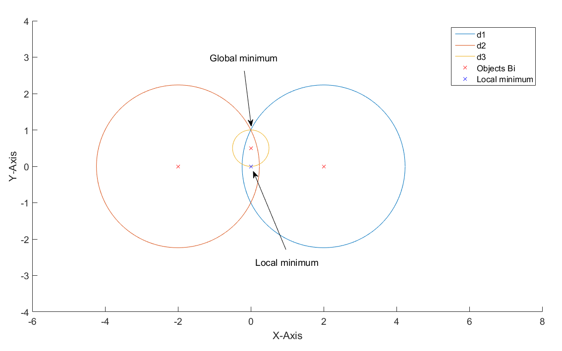
Figure 1 shows three base stations $B_{i}$ at known positions $(a_{i},b_{i},c_{i})$ , and one transponder $T$ at unknown position $(x,y,z)$ . The distances measurements $d_{i}$ between base stations $B_{i}$ and the transponder $T$ are known. The unkown position of the transponder $T$ can be estimated by the known positions of the base stations $B_{i}$ and the distance measurements $d_{i}$ . This data is effected by gaussian noise $e_{i}$ .

Figure 1: The dashed circles with a smaller radius are the true distances between base stations

B_{i}

and transponder

T

. The dashed circles with a radius of

d_{i}+e_{i}

are the false measurements due to noise.

3.1 Mathematical formulation

The distance measurements between the base stations $B_{i}$ and transponder $T$ are defined as

d_{i}=\sqrt{(x_{G}-a_{i})^{2}+(y_{G}-b_{i})^{2}+(z_{G}-c_{i})^{2}}.

1\leq i\leq N

Unknown position of transponder T can be found by solving eq. (1).

•

Objective function one:

F_{1}(x,y,z)\coloneqq\sum_{i=1}^{N}\left[\sqrt{(x-a_{i})^{2}+(y-b_{i})^{2}+(z-c_{i})^{2}}-d_{i}+e_{i}\right]^{2}

(1)

The solving of eq.(1) can be done by non-convex optimization [21] $F_{i}(x,y,z)\rightarrow argmin$ . Alternatively, the non-linear system can be transformed into a linear system [13, 19]. In more complex cases where the positions of base stations $B_{i}$ are unknown this is not possible at all. With regard to future extensions to determining the base station positions as well as the location of the transponder $T$ , this article focuses on finding a solution with a non-convex optimization algorithm.

3.2 Reason for the approach

The objective function (1) is non-linear and non-convex. The optimization of the objective function can cause to convergence to a local minimum $L$ instead the global minimum $G$ (see Table 1). In our approach instead the $F_{1}$ the improved objective function $F_{L1}$ is used. This function has an additional variable $\lambda$ compared to the function $F_{1}$ .

•

Improved objective function one:

F_{L1}(x,y,z,\lambda)\coloneqq\sum_{i=1}^{N}\left[\sqrt{(x-a_{i})^{2}+(y-b_{i})^{2}+(z-c_{i})^{2}+\lambda^{2}}-d_{i}+e_{i}\right]^{2}

(2)

In [20] we have proven that the improved objective function two $F_{L2}(x,y,z,\lambda)\coloneqq\sum_{i=1}^{N}\left[(x-a_{i})^{2}+(y-b_{i})^{2}+(z-c_{i})^{2}+\lambda^{2}-d_{i}^{2}\right]^{2}$ with an additional variable, transforms the local minimum to a saddle point at $\lambda=0$ . Furthermore it was shown that no further local minima exist for $\lambda\neq 0$ at non trivial constellations. The same effect was demonstrated numerically for eq.(1) and eq.(2). The final proof of the hypothesis was provided with the help of the Cauchy-Bunyakovsky-Schwarz inequality[7]. Alternatively, the equation 29 in [20] can also be obtained from the variance $Var(X)=\mathbb{E}\left(\left(X-\mathbb{E}\left(X\right)\right)^{2}\right)=\mathbb{E}\left(X\right)^{2}-\left(\mathbb{E}\left(X\right)\right)^{2}$ . The base stations should have a variance in position higher or equal to zero $0\leq Var(\left\{a_{i}\right\})=\frac{1}{N}\sum_{i=1}^{N}a_{i}^{2}-\left(\frac{1}{N}\sum_{i=1}^{N}a_{i}\right)^{2}=\frac{1}{N}\sum_{i=1}^{N}a_{i}^{2}-\frac{1}{N^{2}}\left(\sum_{i=1}^{N}a_{i}\right)^{2}$ . This leads to the final term $\sum_{i=1}^{N}a_{i}\leq\sqrt{N}\sqrt{\sum_{i=1}^{N}a_{i}{}^{2}}$ . In this article the measurement data is effected by noise, therefore the objective function one (1) is used. In contrast to objective function two is this function statistically correct in presence of noise.

3.3 Two dimensional example

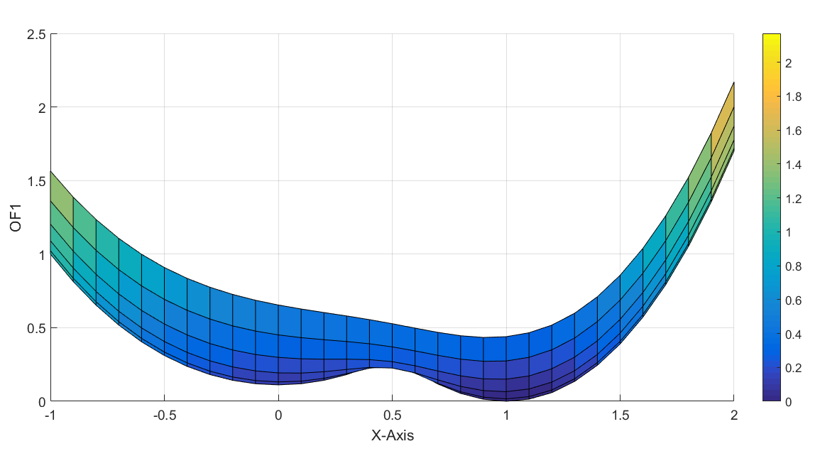
In this section an example is created with known coordinates of the global at $G(1,0)$ , local minimum $L(0,0)$ and no noise. This example has the aim to illustrate the converging steps of the Levenberg-Marquardt algorithm for the $F_{1}$ and $F_{L1}$ . The positions of the local and global minimum leads to the coordinates of base stations $B_{i}$ (See Table 2 ). Figure 2, shows the coordinates of base stations $B_{i}$ , which are located in the center of the circles. And the figure 3, presents the search space of objective function $F_{1}$ .

Table 2: Coordinates of base stations

B_{i}

Base stations X-Position Y-Position $B_{1}$ $0.5$ $0$ $B_{2}$ $0$ $2$ $B_{3}$ $0$ $-2$

Refer to caption — Figure 2: The circles represents the true distance between base stations $B_{i}$ and the global minimum. Blue circle is the distance between base station $B_{2}$ and transponder. Red circle the distance between base station $B_{3}$ and transponder. Yellow circle is the distance between base station $B_{1}$ and transponder .

3.3.1 Local optimization

The Levenberg-Marquardt algorithm uses the derivative to obtain the stepsize, therefore it is important that the initial estimate for the additional variable $\lambda$ is non-zero. Otherwise $\lambda$ remains zero, and $F_{L1}$ is effectively reduced to $F_{1}$ .

Table 3 shows initial estimates of the optimization.

Table 3: Iteration steps of the Levenberg-Marquardt for

F_{1}

and

F_{L1}

$x$ $y$ $\lambda$ Initial estimate 2 -1 1

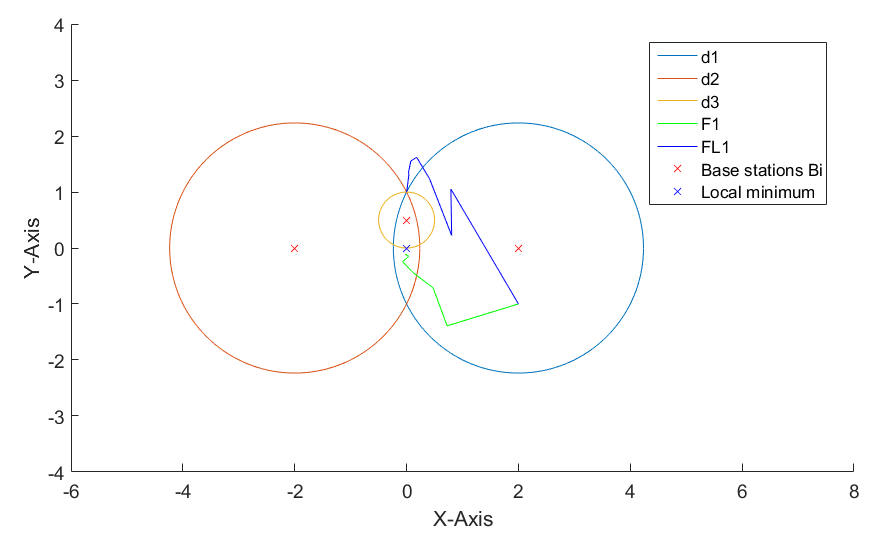
In Figure 3 the result of the optimization can be observed. The blue path shows the steps of the improved objective function $F_{L1}$ , which converge to the global minimum $G(1,0)$ . On the other hand, the original objective function $F_{1}$ represented by the green line, converges to the local minimum $L(0,0)$ .
If the measurement is effect by noise, the residues would be higher than zero at the global minimum. With more additional variables (eq. 4) the error splits up between the additional variables in the manner $\lambda=\sqrt{\sum_{i=1}^{N}\lambda_{i}{}^{2}}$ .

F_{L1}(x,y,z,\lambda_{1})\coloneqq\sum_{i=1}^{N}\left[\sqrt{(x-a_{i})^{2}+(y-b_{i})^{2}+(z-c_{i})^{2}+\lambda_{1}{}^{2}}-d_{i}-e_{i}\right]^{2}

(3)

F_{L2}(x,y,z,\lambda_{2},\lambda_{3})\coloneqq\sum_{i=1}^{N}\left[\sqrt{(x-a_{i})^{2}+(y-b_{i})^{2}+(z-c_{i})^{2}+\lambda_{2}{}^{2}+\lambda_{3}{}^{2}}-d_{i}-e_{i}\right]^{2}

(4)

We assume that the proven hypothesis [20] for the improved objective function two apply as well for the improved objective function one eq.(5).

\left(\frac{\partial^{2}}{\partial\lambda^{2}}F_{L1}\right)(0,0,0,0)=\sum_{i=1}^{N}\frac{\left(\sqrt{a_{i}{}^{2}+b_{i}{}^{2}}-d_{i}+e_{i}\right)}{\sqrt{a_{i}{}^{2}+b_{i}{}^{2}}}<0

(5)

4 Numerical results

The tests were carried out with MALTAB Levenberg-Marquardt algorithm at default settings (Table. 4).

Table 4: Default MATLAB ’Levenberg Marquardt algorithm’ parameter

Value Maximum change in variables for finite-difference gradients Inf Minimum change in variables for finite-difference gradients 0 Termination tolerance on the function value 1e-6 Maximum number of function evaluations allowed 100*numberOfVariables Maximum number of iterations allowed 400 Termination tolerance on the first-order optimality 1e-4 Termination tolerance on x 1e-6 Initial value of the Levenberg-Marquardt parameter 1e-2

The base stations $B_{i}$ , transponder $T$ and initial estimates were randomly generated in a 10x10x10 cube. Unfavorable constellation close to collinearity have been avoided by the requirement that every normalized singular value of the covariance matrix should be higher than $0.1$ .

•

Error term:

E=\sum_{j=1}^{M}\sqrt{(x-x_{G})^{2}+(y-y_{G})^{2}+(z-z_{G})^{2}}

(6)

4.1 Results of the objective function and the improved objective function

In the following section the results of the optimization with a two dimensional $F_{1}$ are presented. Figure 5 shows the error term with different constellations of the four base stations $B_{i}$ . It can be seen that $F_{L1}$ has no outlier for measurement noise smaller than $\sigma\leq 0.01$ . The measurement noise $e_{i}$ effects eq. (5) and could lead to a local minima $\left(\frac{\partial^{2}}{\partial\lambda^{2}}F_{L1}\right)(0,0,0,0)>0$ . Therefore, with higher noise are convergences to local minima also possible for the improved objective function.

Table 5: The examples are based on a 2-D model with 4 base stations

B_{i}

F_{1}

: Objective function one,

F_{L1}

: Improved objective function one, M: Mean error, Sigma: Standard deviation, L: Amount of local minima (Error bigger then

0.5

) .

Noise $\sigma$ Objective function $M\pm\sigma$ L $M\pm\sigma$ without outlier 0.01 $F_{1}$ $1.9139\pm 5.3541$ 1357 $0.0344\pm 0.0286$ 0.01 $F_{L1}$ $0.0357\pm 0.0304$ 0 $0.0357\pm 0.0304$ 0.05 $F_{1}$ $1.8155\pm 5.0454$ 1313 $0.1306\pm 0.0810$ 0.05 $F_{L1}$ $0.1746\pm 0.1505$ 362 $0.1542\pm 0.0986$ 0.1 $F_{1}$ $1.9939\pm 5.1490$ 1900 $0.2250\pm 0.1133$ 0.1 $F_{L1}$ $0.3426\pm 0.2920$ 1743 $0.2419\pm 0.1191$

The mean error without the outlier is higher for the improved objective function one, due to the fact that with more dimensions the ratio between the number of equations with respect to the amount of unknown dimensions and is decreasing.

4.2 Results with more than one additional variable

In figure 6 the results with more than one additional variable can be observed. In contrast to the results of section 4.1, all possible constellations have been used for the lateration. Therefore, in some cases the optimization converges to a local minimum. Regardless the number of additional variables the results are the same, hence it makes no sense to use more than one additional variable.

4.3 Results with restart

The improved objective function $F_{L1}$ has the advantage that it is less effected by local minima. The general objective function has with less dimensions a better noise compensation. Therefore, it makes sense to combine the strength of both functions. In figure 7 we present a method how both effects can be used.

At the beginning of the optimization process the objective function is getting increasing by one additional variable $\lambda$ (step A). In the next step B the optimization is done with the additional variable to minimize the risk to find a local minimum. In step C, the outcome of the optimization is used as initial estimate for the next optimization without the additional variable. Table 6 shows the results of the optimization process with restart. The number of found outlier and mean error is smaller compared to the objective function and the improved objective function.

Table 6: The examples are based on a 2-D model with 4 base stations

B_{i}

F_{1}

: Objective function one,

F_{L1}

: Improved objective function one.

F_{L1}

F_{1}

: Restart of the optimization

F_{L1}

with initial estimates obtained from optimization with

F_{1}

. M: Mean error, Sigma: Standard deviation, L: Amount of local minima (Error bigger then

0.5

)

Noise $M\pm\sigma$ L Noise $\sigma$ without outlier 0.01 $0.0260\pm 0.0175$ 0 $0.0260\pm 0.0175$ 0.05 $0.1302\pm 0.0900$ 61 $0.1269\pm 0.0769$ 0.1 $0.2582\pm 0.1924$ 697 $0.2249\pm 0.1130$

5 Discussion

The presented method shows a huge advantage over the cassic objective function. In [20] we have proven that the improved objective function two $F_{2}$ has a saddle point at the local minimum of objective function two $F_{2}$ . In test scenraios with no or small noise the improved objective function onw $F_{L1}$ never converges into a local minimum. With increasing noise does the improved objective function one $F_{L1}$ lose its ability to avoid local minima. However, the amount of fase converages was ten times lower of $F_{L1}$ compared to $F_{1}$ . On the other side, the function $F_{1}$ has a better noise dumping than $F_{L1}$ . This is due to a better ratio between number of equations to unkown dimensions. The presented method in section 4.3 shows that this disadvange can be overcome with a restart of the optimization with $F_{1}$ with inistial estimates provided by $F_{L1}$ . In any case, it is not necessary to implement more than one additional variable. It is important that the initial estimate of the additional variable is unequal zero. Otherwise gradient-based optimization algorithms like Levenberg-Marquardt would not converge to the additional dimension. In all test scenarios the positions of base stations $B_{i}$ were known. Under the following conditions it is also possible to obtain the solution analytically. In the case of unknown positions of base stations $B_{i}$ and transponders $T_{j}$ it is not feasible anymore. At this point, our approach becomes extremely valuable.

References

[1] J. S. Abel and J. W. Chaffee. Existence and uniqueness of GPS solutions. IEEE Transactions on Aerospace and Electronic Systems, 27(6):952–956, Nov 1991.
[2] David L. Adamy. EW 102: A Second Course in Electronic Warfare. Artech House, Boston London, 2004.
[3] T. Akiyama, M. Sugimoto, and H. Hashizume. Light-synchronized acoustic ToA measurement system for mobile smart nodes. In 2014 International Conference on Indoor Positioning and Indoor Navigation (IPIN), pages 749–752, Oct 2014.
[4] Egon Balas. Projection, lifting and extended formulation in integer and combinatorial optimization. Annals of Operations Research, 140(1):125, 2005.
[5] S. Bancroft. An algebraic solution of the GPS equations. IEEE Transactions on Aerospace and Electronic Systems, AES-21(1):56–59, Jan 1985.
[6] P. Benevides, G. Nico, J. Catalão, and P. M. A. Miranda. Analysis of galileo and GPS integration for GNSS tomography. IEEE Transactions on Geoscience and Remote Sensing, 55(4):1936–1943, April 2017.
[7] V.I Bityutskov. Bunyakovskii inequality. Encyclopedia of Mathematics, 2001.
[8] P. P. Bogdanov, A. V. Druzhin, A. E. Tiuliakov, and A. Y. Feoktistov. GLONASS time and UTC(SU). In 2014 XXXIth URSI General Assembly and Scientific Symposium (URSI GASS), pages 1–3, Aug 2014.
[9] A. E. Cetin, A. Bozkurt, O. Gunay, Y. H. Habiboglu, K. Kose, I. Onaran, M. Tofighi, and R. A. Sevimli. Projections onto convex sets (POCS) based optimization by lifting. In 2013 IEEE Global Conference on Signal and Information Processing, pages 623–623, Dec 2013.
[10] J. Chaffee and J. Abel. On the exact solutions of pseudorange equations. IEEE Transactions on Aerospace and Electronic Systems, 30(4):1021–1030, Oct 1994.
[11] Don Douglass. GPS instant navigation : A practical guide from basics to advanced techniques by kevin monahan. Fine Edge Productions, 1998.
[12] H. Fawzi et al. Equivariant semidefinite lifts of regular polygons. In DOI: 10.1287/moor.2016.0813, 2014.
[13] Juri Sidorenko et. al. Improved linear direct solution for asynchronous radio network localization (RNL). In 2017 Pacific Positioning, Navigation and Timing technology (PNT), 2017.
[14] V. Nambiar et al. SDR based indoor localization using ambient WiFi and GSM signals. In 2017 International Conference on Computing, Networking and Communications (ICNC), pages 952–957, Jan 2017.
[15] H. Hmam. Quadratic optimisation with one quadratic equality constraint. Electronic Warfare and Radar Division, 2010.
[16] Shih-Mim Liu and G. P. Papavassilopoulos. Algorithms for globally solving d.c. minimization problems via concave programming. American Control Conference, 1995.
[17] A. Marquez, B. Tank, S. K. Meghani, S. Ahmed, and K. Tepe. Accurate UWB and IMU based indoor localization for autonomous robots. In 2017 IEEE 30th Canadian Conference on Electrical and Computer Engineering (CCECE), pages 1–4, April 2017.
[18] Jorge J. Moré. The Levenberg-Marquardt algorithm: Implementation and theory. In In G. A. Watson (ed.): Numerical Analysis. Dundee 1977, Lecture Notes Math. 630, 1978, S. 105-116, 1978.
[19] J. Sidorenko, N. Scherer-Negenborn, M. Arens, and E. Michaelsen. Multilateration of the local position measurement. In 2016 International Conference on Indoor Positioning and Indoor Navigation (IPIN), pages 1–8, Oct 2016.
[20] Juri Sidorenko, Leo Doktorski, Volker Schatz, Norbert Scherer-Negenborn, and Michael Arens. Improved time of arrival measurement model for non-convex optimization. arXiv:1801.03266.
[21] Stephen M Stigler. Gauss and the invention of least squares. The Annals of Statistics, 1981.
[22] M. Vossiek, R. Roskosch, and P. Heide. Precise 3-d object position tracking using FMCW radar. In 1999 29th European Microwave Conference, volume 1, pages 234–237, Oct 1999.