Parton distributions and asymmetry
induced by anomalous photon-quark coupling
Abstract
Abstract: In the spectator models of the nucleon with scalar and axial-vector diquarks, we show that the effect of Pauli coupling in photon-quark vertex to the parton distribution functions (PDFs) of nucleon and azimuthal asymmetry in the unpolarized semi-inclusive deep inelastic scattering (SIDIS). This anomalous coupling gives obvious contribution to unpolarized and polarized PDFs, and also leads to a azimuthal asymmetry proportional to the squared Pauli form factor, due to the helicity flip of the struck quark. After determining the model parameters by fitting PDFs to the global fits, this new distribution for asymmetry is given numerically. In the framework of transverse momentum dependence (TMD), we find that it is positive and of a few percent in the kinematical regime of HERMES and COMPASS collaborations, in the same order of magnitude with Cahn effect.
pacs
12.39.-x, 13.60.Hb, 13.88.+eI Introduction
The semi-inclusive deep inelastic scattering (SIDIS) not only plays an essential role in studying the parton distribution functions (PDF) of nucleon, but also its azimuthal asymmetries are important observables related to the transverse spin of quarks inside target hadrons [1]. Two azimuthal moments are present in the unpolarized differential cross sections, with the angular dependence of and , respectively (here and afterwards is the azimuthal angle of produced hadron in the scattering plane). Two main mechanisms for the origin of these asymmetries are usually considered when QCD factorization is applicable. One of them involves the convolution of Boer-Mulders function [2], which measures the transverse polarization asymmetry of quarks inside an unpolarized hadron, and the spin-dependent Collins fragmentation function (FF) of the produced hadron [3, 4]. The other one is in terms of Cahn effect, related to the non-collinear transverse-momentum kinematics. While the former effect is the leading twist one, the latter is kinematically of higher twist. These functions should be either calculated within some phenomenological models [7, 6, 5, 8] or be extracted directly from experiments [9, 10, 11, 12, 13, 14, 16, 15, 17, 18, 19, 20, 21].
Dirac vector coupling is widely explored in the quark electromagnetic and chromomagnetic current, but the tensor coupling with respect to anomalous Pauli form factor is less recognized. These Pauli couplings can flip the quark helicity, which is one of the important ingredients to induce single-spin asymmetries (SSA) in SIDIS. It was found that the Pauli couping in quark-gluon vertex from various sources leads to a large SSA in quark-quark scattering [22]. In the hadronic level, possible role of the Pauli-type soft quark-gluon interaction on SSAs in SIDIS was investigated in spectator model [23]. Within the same model adopting the scalar and axial-vector diquark models for the nucleon, it was recently demonstrated that Pauli couplings in both quark-photon and quark-gluon vertices produce considerable SSA in SIDIS, whose azimuthal dependencies are the same as that usually called the Collins and Sivers effects [24]. Alternatively approaches, e.g. instanton background field [25], MIT bag model [26] and single instanton approximation [27], arrive at similar conclusions. This remarkable mechanism would be promising for our understanding of the large SSAs observed in high energy hadronic reactions and in SIDIS [1].
The Pauli couplings can be originated from instantons, a small size strong gluonic fluctuation in the QCD vacuum [28, 29]. These non-trivial topological structure of QCD equations generate a very large quark chromomagnatic moment, directly resulting into the Pauli coupling in quark-gluon vertex [30]. It was revealed that this anomalous interaction would play important role in gluon distributions in the nucleon [31], in quark-gluon plasma [32], in high energy elastic scattering [33] and reaction [34]. In these analyses it was suggested that this quark-gluon interaction would cause the explicit breakdown of transverse-momentum-dependent (TMD) factorization. In addition, the instantons would also give rise to the Pauli coupling in quark–photon vertex, as illustrated within the nonperturbative approach [35, 36]. The instanton liquid model [28, 29] is widely implemented in the qualitative calculations.
The purpose of this paper is to consider what specifical effects the Pauli coupling of quark-photon interaction may have on PDFs and unpolarized SIDIS. The contribution of this interaction are expected to be complementary to the Dirac couplings. In Sec. II we give our analytical results of TMD PDFs in spectator models and try to extract the model parameters from the global PDF fits. In Sec. III, we give our new asymmetry in the framework of TMD factorization and compare it to the Cahn effect. We conclude briefly in Sec. IV.
II TMD Parton Distributions in spectator models

In this work we employ the parton model of nucleon by using the spectator model with scalar and axial-vector diquarks [37], as depicted in Fig 1. We introduce a Pauli coupling besides the conventional Dirac coupling at the vertex between the struck quark and the virtual photon [35]:
| (1) |
with being the constitute quark mass. The and are Dirac and Pauli form factors as a function of photon virtuality , respectively. The perturbative and non-perturbative QCD contributions to the Dirac and Pauli form factor have been calculated with several methods (see [35, 38] and references therein). It should be noted that the non-perturbative interaction enters into the model only through above quark-photon vertex. It does not affect the kinematical relationships of involved momenta, but it would influence the virtualities of internal lines of hard scattering. As a matter of fact, it can be easily checked that the Pauli coupling present in Eq. (1) is very moderately dependent on and roughly follow the order of the usual Diral vector coupling in the instanton liquid model because of the small instanton size (see Eq. (44) hereafter in Sec. III). So it is naively expected this new vertex does not break the TMD factorization between the hard and soft part of SIDIS, and the standard treatment of the convolution between TMD PDFs and FFs can be still used here in the factorization framework [39, 40]. Moreover, in our previous calculation of the SSA in SIDIS induced by the Pauli couplings [24], terms which obviously violate order counting in TMD factorization are not present. There we also found that the Pauli coupling in quark-gluon vertex from instanton liquid model does provide appropriate regularization of the loop integrals from final state interaction. In Ref. [26], the Sivers function resulted from this Pauli coupling is successfully calculated by the correlator in terms of gauge links, adopting the same instanton model with ours and the quark wave functions from MIT bag model. A rigorous proof of the TMD factorization theorem with regard to the Pauli couplings would follow the framework recently proposed within the scalar diquark model in our interested kinematical range and is waiting for future exploration [41].
The nucleon-quark-diquark vertices are chosen to be
| (2) |
where the and are couplings in proton-quark-scalar diquark vertex and proton-quark-axial-vector diquark vertex, respectively. Then the amplitudes of Born diagram presented in Fig. 1 are straightforwardly written as
| (3) | |||||
| (4) | |||||
for the scalar and axial-vector diquark models, respectively. Here the and are helicities of the photon and axial-vector diquark, respectively. The and label the helicities of initial and final quarks, respectively. The helicity amplitudes are obeying the relations
| (5) |
Following the approach of Hoyer and Jarvinen [23], we work in a coordinate system where the target proton is at rest (laboratory frame) and the virtual photon momentum is along the +z axis, e.g. the momenta of photon, proton and struck quark read [23]
| (6) |
with being the photon energy, the proton mass and the Bjorken variable, respectively. Here we describe a generic four-vector as and its square . We use as the magnitude of . The polarization vectors of photon and axial-vector diquark are defined as
| (7) | |||||
| (8) |
where the transversality condition, e.g. , is respected. For simplicity, we define,
| (9) |
with and being the diquark mass. After some algebraic caculation, in the limit of at fixed , the helicity amplitudes for the scalar diquark model are found to be
| (10) | |||||
| (11) |
with and . For the axial-vector diquark model, the full set of amplitudes is
| (12) | |||||
| (13) | |||||
| (14) | |||||
| (15) | |||||
| (16) | |||||
| (17) | |||||
| (18) | |||||
| (19) |
The differential cross section of unpolarized and longitudinal polarized DIS is given in terms of the amplitude at tree order in Fig 1(a):
| (20) | |||||
with the Bjorken variables being the fraction of the beam energy carried by the virtual photon. The depolarization factor is the ratio of longitudinal and transverse photon flux,
| (21) |
with . Above we have used the leptonic tensor in the helicity basis
| (22) |
Here is the azimuthal angle of the lepton . After some formalism manipulation, we have for the scalar diquark model
| (23) | |||||
| (24) | |||||
| (25) | |||||
For axial-vector diquark model, we have
| (26) | |||||
| (27) | |||||
| (28) | |||||
As expected, the distributions and return back to the results of conventional diquark models [6] when is approaching zero. Besides, an asymmetric term with definite angular distribution are generated by the photon-quark Pauli couplings. If we use the Trento convention [42], which uses the angle between the hadron and lepton planes
| (29) |
Then the angular dependence of are , which is identical to those of the Cahn and Boer-Mulders effect. Its physical origin is, however, quite different from the original azimuthal asymmetries in SIDIS. As can be seen in Eq. (24) and Eq. (26), the magnitudes of are proportional to the squared Pauli form factor , which is from non-perturbative contribution and could be explicitly calculated by various phenomenological models, e.g. the instanton liquid model for nontrivial topological structure of QCD vacuum [35]. It should be noted that the Pauli couplings introduced in Eq. (44) are dependent, which will discussed in detail in Sec. III.
In our above calculation, we neglect the form factors which are introduced to smoothly suppress the contribution of high transverse momentum. Here we introduce conventional dipolar form factors in the photon-quark couplings:
| (30) |
We can read the unpolarized and helicity parton distribution functions (PDFs) from Eq. (23), Eq. (25), Eq. (26), and Eq. (28):
| (31) | |||||
| (32) | |||||
| (33) | |||||
| (34) |
which return back to the results of conventional diquark model [23] when . We can also define a new distribution function alike to Cahn effect by Eq. (24) and Eq. (26) as
| (35) | |||||
| (36) |
In above equations, are the normalization factors determined by
| (37) |
The -integrated results , and are given in the Appendix A.
| Fit-I | Fit-II | |
|---|---|---|
| (GeV) | 0.3† | 0.3† |
| (GeV) | 0.769 0.038 | 0.829 0.025 |
| (GeV) | 1.5† | 1.5† |
| (GeV) | 0.857 0.065 | 0.921 0.007 |
| (GeV) | 0.683 0.028 | 0.545 0.017 |
| (GeV) | 0.767 0.030 | 0.509 0.025 |
| (GeV) | 0.434 0.027 | 0.385 0.006 |
| 0.445 0.048 | 0.657 0.061 | |
| 1.245 0.060 | 1.112 0.089 | |
| 0.639 0.011 | 0.662 0.012 | |
| 0.0† | 0.921 0.117 | |
| 8.51 | 4.12 |
After determining the parameters of the model by fitting known unpolarized and polarized distribution functions and , we can predict the numerical results of our model for the asymmetry. To perform the fit, we need to relate the functions and in terms of diquark types in the model, to the functions and with regard to quark flavors in the global fits. We write them generally as [7, 6]
| (38) | |||||
| (39) |
which should be generalized to the case of and . Here we discriminate the two isospin states of the vector diquark, namely for the diquark and for the diquark. We have , and under the SU(4) symmetry. However, since SU(4) symmetry is no longer strictly preserved in the spectator model of nucleon, we treat these coefficients instead as free parameters. We have checked that the results are not sensitive to the values of the masses of constituent quark and diquark , so we fix them to be 0.30 GeV and 1.5 GeV. We have in total nine free parameters for the model.
In order to reproduce the parametrizations of PDFs extracted from experimental data, we have to choose a proper scale at which diquark models are probably appropriate. Following the arguments in literatures [7, 6], a very low scale seems to be favored, so lowest possible value of scale is used in the literature, e.g. GeV2 [6] and GeV2 [7]. Only a few PDFs of global fit are at hand in such low range and most of them are usually applicable above 1.0 GeV2, e.g. CT14 [43], MMHT2014 [44], NNPDF [45], and ABM11 [46]. We fit our model parameters to leading order GRV1998 [47] and GRSV2000 [48] parametrization at = 0.26 GeV2 for and , respectively. We assign a constant relative error of 5.0% to based on comparisons with HERAPDF [49] and IMParton [50, 51] under the same . We allocate a relative error of 20.0% to in view of confronting with DNS2005 [52] and DSSV2010 [53] (see Ref [54, 55] for a detailed comparison of various ).
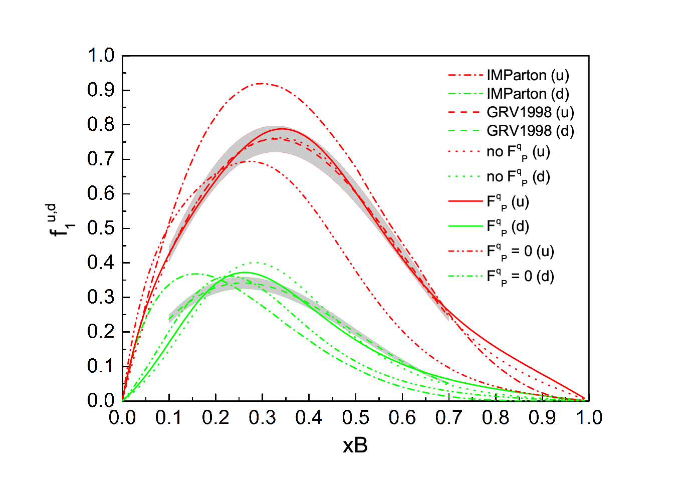
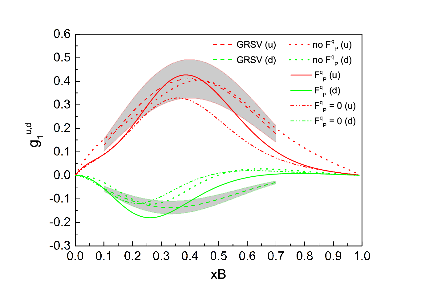
The fit results are shown in Fig. 2 and Fig. 3 for and , respectively. The extracted parameters are shown in Tab. 1. In Fit-I, we use the conventional model, in which there is no Pauli coupling in photon-guark vertex, e.g setting in the fit. We achieve a good agreement except for the . The fitted goes to positive values in the range of around , while it is negative in the full range in GRSV2000. This conclusion has been found before in Ref. [6]. In Fit-II, we use the full model with at = 0.26 GeV2 as free parameter. In spite of the high because we choose small relative errors for , the agreement is acceptable for all the PDFs and the overall is promoted significantly. The fit of is as good as that in Fit-I, and the is slightly improved. Though the description of becomes a little worse in Fit-II, the is much better from to . The contribution of Pauli coupling is significant above , as can be seen in Fig. 2 and Fig. 3, when we turn off it in the fit results of Fit-II.
In Fig. 4, we give the predicted distributions at GeV2 in our model. The magnitude of quark distribution is much bigger than that of quark, though the their shape is close to each other. The maximum for both distributions is around at .

III Comparism to data of asymmetry
The asymmetries in SIDIS off hydrogen, deuterium and 3He targets have already been extensively explored by EMC [56], ZEUS [57, 58], HERMES [60, 59], COMPASS [62, 63, 64, 61] collaborations and at JLab [67, 66, 65]. Since both HERMES [59] and COMPASS [61] collaborations have measured the SIDIS off unpolarized proton for charged unidentified hadrons () among final particles but under slightly different , here we try to compare our new asymmetry in Eq. (35) and Eq. (36) with the parameters in Tab. 1 to these data, together with Cahn effect. We do not aim to a full analysis of the azimuthal asymmetry based on all released data, because it is beyond the scope of present paper. Attempts to this direction can be found in a series of publications [5, 11, 12, 13, 14, 16, 15]. For the same reason, we also do not investigate Boer-Mulders distribution [2] here, for which Collins FFs of the production hadron should be introduced [3, 4].
In parton model, the SIDIS differential cross sections are expressed as the convolution of TMD PDFs and FFs [5, 11, 12, 13]:
| (40) | |||||
where the sum runs over the quark favor . We denote by the transverse momentum of the final hadron , and by the transverse momentum of with respect to the direction of the fragmenting quark. The is well recognized in the Gaussian form:
| (41) |
We adopt the unpolarized DSS FFs at leading order for [68] with 0.2 GeV2 [9, 13]. The results do not change much if the SKMA FFs [69] are used instead.
Similarly, the contribution of the distribution to the asymmetry can be defined as,
| (42) | |||||
The Cahn effect to asymmetry can be obtained by substituting the with the following function in above definition [70, 71]:
| (43) |
with . As the only known one of the twist-4 effects, it is at the order of and hence it is controversial when we use the identical kinematical relations and factorization as the leading twist (see discussions in Refs [12, 13]). We have to leave these debate behind at present before these problems are completely resolved from theoretical side.
The extracted value of is close to 1.0 in Sec. II. This is in fact roughly compatible with the calculation in the instanton model [36], where it is found that the dependence of Pauli coupling can be parameterized very well by
| (44) |
with the instanton size fm. As a result our new distribution is at the order of and would suffer the same kinematical and dynamical problems with the case of Cahn effect as mentioned above. Moreover, the decreases very rapidly below = 1.0 GeV2 and approaches a constant above 2.0 GeV2. As a result, it is expected that the strength of the new asymmetry is enlarged in very low . However, the data in this range is unavailable. The average of HERMES [59] and COMPASS [61] measurements are about 2.5 and 3.0 GeV2, respectively 11 1 There is strong correlation between variables and (and thus between and ), but we put aside this problem at present and it should pay caution to the sub-figures with variable in Fig. 5 and Fig. 6. In principle we need to evolute our distributions from to the experimental one. For the reason that the evolution of these distributions is not firmly established [17], we only simply use the value of at experimental , determined by Eq. (44) during our comparison. This leads to a reduction of about one order of magnitude of compared to that at . It should be mentioned here that the data of EMC [56] and ZEUS [57, 58] are measured in very high , so the contribution of both Cahn effect and our new distribution to asymmetry are anticipated to be negligible.
The measured asymmetry in experiment is defined as
| (45) |
where the integrations are performed over the measured kinematical ranges of , , and , which can be found in the papers of HERMES [59] and COMPASS [61] collaborations. The detailed formalism of integrations are present widely in the literatures [13, 16].
Our calculated results are shown in Fig. 5 and Fig. 6, together with the corresponding data. As can be seen, the magnitude of the asymmetry induced by our new distribution is of a few percent and comparable to the Cahn effect in various kinematical ranges. The new and Cahn asymmetry are both flavor blind and positive for inclusive production while Boer-Mulders effect is flavor dependent. Our asymmetry seems to be bigger than Cahn effect in the kinematic range of the COMPASS measurement, as displayed in Fig. 6. Another feature is that our new asymmetry is more weakly dependent on the kinematical variables than Cahn effect. Especially, it does not vanish when is approaching zero, as Cahn effect does. The new asymmetry only begins to drop to zero when is smaller than 0.2, as can be seen in Fig. 5. We arrive at the analogous conclusion for the identified charged pions and kaons produced by SIDIS off nucleon, hydrogen and deuterium targets.
It is concluded that the behavior of the COMPASS data seems to be incompatible with the corresponding behavior of HERMES data by Barone [13]. Our new distribution in Eq. (35) and Eq. (36) as functions of kinematical variables is unlike Cahn effect, which is clearly illustrated in Fig. 5 and Fig. 6. So it would be helpful for the understanding this inconsistency phenomenologically. A reliable extract of Cahn and Boer-Mulders effects from experimental data should be done by considering the effect from our distribution .


IV Conclusion
In summary, we investigate the role of Pauli coupling in photon-quark vertex to SIDIS. In the calculation we utilize the scalar and axial-vector diquark models for the target nucleon. Our analytical formalism unveil that obvious -dependence is introduced into PDFs by this additional photon-quark vertex. We determine the Pauli coupling in the scale of = 0.26 GeV2 by fitting to the global fit of the PDFs. The determined value of Pauli coupling agrees approximately with the prediction from instanton model. The numerical results have shown that Pauli coupling contributes considerably to the unpolarized and polarized PDFs in the low-.
Furthermore, we demonstrate that the Pauli coupling in photon-quark vertex can cause the helicity flip of the struck quark, leading to a new positive asymmetry in SIDIS. The magnitude of the asymmetry is proportional to the squared Pauli coupling, which introduce a significant dependence into its evolution. If admitting this dependence expediently from instanton model, the given asymmetry is in the same level with Cahn effect and of the order of a few percent in size within the HERMES and COMPASS kinematics. In other words, the magnitude of this new asymmetry is expected to be larger than that of Cahn effect in the range of 2.0 GeV since it has a stronger dependence than Cahn effect. So the measurement of dependence of the asymmetry is crucial to disentangle higher-twist effects and our new asymmetry.
The important observation is that the asymmetry at low range should be explored systematically by including the effect from our distribution, together with Cahn and Boer-Mulders effects. The available data of asymmetry in SIDIS do not allow yet a full extraction of Boer-Mulders function due to the present kinematics which is still dominated by the low- region. It is already found that the higher-twist contributions are of great significance and strongly affect the results of the fits [11, 12]. The multidimensional data for the multiplicities released by HERMES [59] and COMPASS [61] collaborations have big uncertainties and they are also not sufficient for a full determination of Boer-Mulders function [13]. Because contribution of our new asymmetry is sizable, it is more difficult for the experimental scrutiny of Boer-Mulders function. The future electron-ion colliders are anticipated to measure the asymmetry in higher range where both our new asymmetry and other high twist contribution, e.g. Cahn effect, are expected to be small. We do not find any contribution of Pauli coupling to azimuthal modulation, so the condition would be more simple there for the determination of the Boer-Mulders function.
It has been discovered that Pauli couplings in both photon-quark and photon-gluon vertices are contributing to the angular dependence of SSA observables in polarized SIDIS [24, 23]. Our calculations here complement earlier studies and accomplish a full picture about the influence of the helicity nonconservation interactions on SIDIS measurements. The instantons are a possible underlying mechanism for these novel interactions and they give explicit dependence of the corresponding couplings. Other optional approaches [72, 73], e.g. Dyson-Schwinger equations with the nonperturbative quark and gluon propagators [74], are waiting for extending to nonzero photon virtuality before a feasible comparison of different models.
Acknowledgements.
It is gratefully acknowledged for the enlightening discussions with Prof. Vicente Vento, Prof. Nikolai Kochelev and Dr. Nikolai Korchagin at the initial stage of this work. We thank Dr. Ruilin Zhu and Dr. Wenjuan Mao for help to polish the paper. We would like to thank Prof. R. Sassot for send us the files of DSS fragmentation functions, and Dr. Rong Wang for the IMParton PDF files. This work was supported by the National Natural Science Foundation of China (Grant No. 11405222).*
Appendix A -integrated distributions
Her we list the -integrated results , and obtained in the context of our spectator diquark model:
| (46) | |||||
| (47) | |||||
| (48) | |||||
| (49) | |||||
| (50) | |||||
| (51) |
References
- [1] V. Barone, F. Bradamante and A. Martin, Prog. Part. Nucl. Phys. 65, 267 (2010).
- [2] D. Boer and P. J. Mulders, Phys. Rev. D 57, 5780 (1998)
- [3] J. C. Collins, Nucl. Phys. B 396, 161 (1993).
- [4] J. C. Collins, Phys. Lett. B 536, 43 (2002).
- [5] V. Barone, Z. Lu and B. Q. Ma, Phys. Lett. B 632, 277 (2006)
- [6] A. Bacchetta, F. Conti and M. Radici, Phys. Rev. D 78, 074010 (2008)
- [7] A. Bacchetta, A. Schaefer and J. J. Yang, Phys. Lett. B 578, 109 (2004)
- [8] L. P. Gamberg, G. R. Goldstein and M. Schlegel, Phys. Rev. D 77, 094016 (2008)
- [9] M. Anselmino, M. Boglione, U. D’Alesio, A. Kotzinian, F. Murgia and A. Prokudin, Phys. Rev. D 71, 074006 (2005)
- [10] M. Anselmino, M. Boglione, J. O. Gonzalez Hernandez, S. Melis and A. Prokudin, JHEP 1404, 005 (2014)
- [11] V. Barone, A. Prokudin and B. Q. Ma, Phys. Rev. D 78, 045022 (2008)
- [12] V. Barone, S. Melis and A. Prokudin, Phys. Rev. D 81, 114026 (2010)
- [13] V. Barone, M. Boglione, J. O. Gonzalez Hernandez and S. Melis, Phys. Rev. D 91, no. 7, 074019 (2015)
- [14] B. Zhang, Z. Lu, B. Q. Ma and I. Schmidt, Phys. Rev. D 78, 034035 (2008)
- [15] Z. Lu and I. Schmidt, Phys. Rev. D 81, 034023 (2010)
- [16] B. Zhang, Z. Lu, B. Q. Ma and I. Schmidt, Phys. Rev. D 77, 054011 (2008)
- [17] M. G. Echevarria, A. Idilbi, Z. B. Kang and I. Vitev, Phys. Rev. D 89, 074013 (2014)
- [18] M. Boglione, S. Melis and A. Prokudin, Phys. Rev. D 84, 034033 (2011)
- [19] B. Pasquini and P. Schweitzer, Phys. Rev. D 83, 114044 (2011)
- [20] P. Schweitzer, T. Teckentrup and A. Metz, Phys. Rev. D 81, 094019 (2010)
- [21] Z. Wang, X. Wang and Z. Lu, Phys. Rev. D 95, no. 9, 094004 (2017)
- [22] N. Kochelev and N. Korchagin, Phys. Lett. B 729, 117 (2014)
- [23] P. Hoyer and M. Jarvinen, JHEP 0510, 080 (2005)
- [24] X. Cao, N. Korchagin, N. Kochelev and P. Zhang, Phys. Rev. D 96, no. 11, 114010 (2017)
- [25] D. Ostrovsky and E. Shuryak, Phys. Rev. D 71, 014037 (2005)
- [26] I. O. Cherednikov, U. D’Alesio, N. I. Kochelev and F. Murgia, Phys. Lett. B 642, 39 (2006)
- [27] Y. Qian and I. Zahed, Annals Phys. 374, 314 (2016)
- [28] T. Schäfer and E. V. Shuryak, Rev. Mod. Phys. 70, 323 (1998)
- [29] D. Diakonov, Prog. Part. Nucl. Phys. 51, 173 (2003)
- [30] N. I. Kochelev, Phys. Lett. B 426, 149 (1998)
- [31] N. Kochelev, H. J. Lee, B. Zhang and P. Zhang, Phys. Lett. B 757, 420 (2016)
- [32] N. Kochelev, H. J. Lee, Y. Oh, B. Zhang and P. Zhang, Phys. Rev. C 93, no. 2, 021901 (2016)
- [33] N. Kochelev and N. Korchagin, Phys. Rev. D 89, 034028 (2014)
- [34] N. Kochelev, H. J. Lee, B. Zhang and P. Zhang, Phys. Rev. D 92, 034025 (2015)
- [35] N. I. Kochelev, Phys. Lett. B 565, 131 (2003)
- [36] B. Zhang, A. Radzhabov, N. Kochelev and P. Zhang, Phys. Rev. D 96, no. 5, 054030 (2017)
- [37] R. Jakob, P. J. Mulders and J. Rodrigues, Nucl. Phys. A 626, 937 (1997)
- [38] A. E. Dorokhov and I. O. Cherednikov, Phys. Rev. D 67, 114017 (2003)
- [39] X. d. Ji, J. p. Ma and F. Yuan, Phys. Rev. D 71, 034005 (2005)
- [40] A. Bacchetta, M. Diehl, K. Goeke, A. Metz, P. J. Mulders and M. Schlegel, JHEP 0702, 093 (2007)
- [41] E. Moffat, W. Melnitchouk, T. C. Rogers and N. Sato, Phys. Rev. D 95, no. 9, 096008 (2017)
- [42] A. Bacchetta, U. D’Alesio, M. Diehl and C. A. Miller, Phys. Rev. D 70, 117504 (2004)
- [43] S. Dulat et al., Phys. Rev. D 93, no. 3, 033006 (2016)
- [44] L. A. Harland-Lang, A. D. Martin, P. Motylinski and R. S. Thorne, Eur. Phys. J. C 75, no. 5, 204 (2015)
- [45] R. D. Ball et al. [NNPDF Collaboration], JHEP 1504, 040 (2015)
- [46] S. Alekhin, J. Blumlein and S. Moch, Phys. Rev. D 86, 054009 (2012)
- [47] M. Glück, E. Reya and A. Vogt, Eur. Phys. J. C 5, 461 (1998)
- [48] M. Glück, E. Reya, M. Stratmann and W. Vogelsang, Phys. Rev. D 63, 094005 (2001)
- [49] H. Abramowicz et al. [H1 and ZEUS Collaborations], Eur. Phys. J. C 75, no. 12, 580 (2015)
- [50] X. Chen, J. Ruan, R. Wang, P. Zhang and W. Zhu, Int. J. Mod. Phys. E 23, no. 10, 1450057 (2014)
- [51] X. Chen, J. Ruan, R. Wang, P. Zhang and W. Zhu, Int. J. Mod. Phys. E 23, no. 10, 1450058 (2014)
- [52] D. de Florian, G. A. Navarro and R. Sassot, Phys. Rev. D 71, 094018 (2005)
- [53] D. de Florian, R. Sassot, M. Stratmann and W. Vogelsang, Phys. Rev. D 80, 034030 (2009)
- [54] M. Hirai et al. [Asymmetry Analysis Collaboration], Phys. Rev. D 69, 054021 (2004)
- [55] F. Taghavi-Shahri, H. Khanpour, S. Atashbar Tehrani and Z. Alizadeh Yazdi, Phys. Rev. D 93, no. 11, 114024 (2016)
- [56] M. Arneodo et al. [European Muon Collaboration], Z. Phys. C 34, 277 (1987).
- [57] J. Breitweg et al. [ZEUS Collaboration], Phys. Lett. B 481, 199 (2000)
- [58] S. Chekanov et al. [ZEUS Collaboration], Eur. Phys. J. C 51, 289 (2007)
- [59] A. Airapetian et al. [HERMES Collaboration], Phys. Rev. D 87, no. 1, 012010 (2013)
- [60] F. Giordano et al. [HERMES Collaboration], J. Phys. Conf. Ser. 295, 012092 (2011)
- [61] C. Adolph et al. [COMPASS Collaboration], Nucl. Phys. B 886, 1046 (2014)
- [62] G. Sbrizzai [COMPASS Collaboration], J. Phys. Conf. Ser. 295 (2011) 012043
- [63] W. Kafer [COMPASS Collaboration], arXiv:0808.0114 [hep-ex].
- [64] A. Bressan [COMPASS Collaboration], arXiv:0907.5511 [hep-ex].
- [65] X. Yan et al. [Jefferson Lab Hall A Collaboration], Phys. Rev. C 95, no. 3, 035209 (2017)
- [66] M. Osipenko et al. [CLAS Collaboration], Phys. Rev. D 80, 032004 (2009)
- [67] H. Mkrtchyan et al., Phys. Lett. B 665, 20 (2008)
- [68] D. de Florian, R. Sassot and M. Stratmann, Phys. Rev. D 75, 114010 (2007)
- [69] M. Soleymaninia, A. N. Khorramian, S. M. Moosavi Nejad and F. Arbabifar, Phys. Rev. D 88, no. 5, 054019 (2013)
- [70] R. N. Cahn, Phys. Lett. 78B, 269 (1978).
- [71] R. N. Cahn, Phys. Rev. D 40, 3107 (1989).
- [72] Z. Lu and I. Schmidt, Phys. Rev. D 75, 073008 (2007)
- [73] A. Bacchetta and M. Radici, Phys. Rev. Lett. 107, 212001 (2011)
- [74] L. Chang, Y. X. Liu and C. D. Roberts, Phys. Rev. Lett. 106, 072001 (2011)