Preprint CERN-TH-2017-269
Same-sign WW scattering at the LHC:
can we discover BSM effects before discovering new states?
Jan Kalinowski,a,b
Paweł Kozów,a Stefan Pokorski,a
Janusz Rosiek,a Michał Szleperc
and
Sławomir Tkaczyk d
a Institute of Theoretical Physics, Faculty of Physics, University of Warsaw,
ul. Pasteura 5, PL–02–093 Warsaw, Poland
b CERN, Theoretical Physics Department,
CH-1211 Geneva 23, Switzerland
c National Center for Nuclear Research, High Energy Physics Department,
ul. Hoża 69, PL-00-681, Warsaw, Poland
d Fermi National Accelarator Laboratory,
Batavia, IL 60510, USA
Abstract
It is possible that measurements of vector boson scattering (VBS) processes at the LHC will reveal disagreement with Standard Model predictions, but no new particles will be observed directly. The task is then to learn as much as possible about the new physics from a VBS analysis carried within the framework of the Effective Field Theory (EFT). In this paper we discuss issues related to the correct usage of the EFT when the invariant mass is not directly accessible experimentally, as in purely leptonic decay channels. Strategies for future data analyses in case such scenario indeed occurs are proposed.
1 Introduction and strategy
Searches for deviations from Standard Model (SM) predictions in processes involving interactions between known particles are a well established technique to study possible contributions from Beyond the Standard Model (BSM) physics. In this paper we address the question how much we can learn about the scale of new physics and its strength using the Effective Field Theory (EFT) approach to scattering if a statistically significant deviation from the SM predictions is observed in the expected LHC data for the process . Our specific focus is on the proper use of the EFT in its range of validity. With this in mind, we discuss the practical usefulness of the EFT language to describe vector boson scattering (VBS) data and whether or not this can indeed be the right framework to observe the first hints of new physics at the LHC.
The EFT is in principle a model independent tool to describe BSM physics below the thresholds for new states. One supplements the SM Lagrangian by higher dimension operators
| (1.1) |
where the ’s are some “coupling constants” and ’s are the decoupled new mass scales. The mass scale is a feature of the UV completion of the full theory and thus is assumed common to all the coefficients
| (1.2) |
which are free parameters because the full theory is unknown. One should stress that the usefulness of any EFT analysis of a given process relies on the assumption that only few terms in the expansion of Eq. (1.1) give for that process an adequate approximation to the underlying UV theory. The necessary condition obviously is that the energy scale of the considered process, . However, the effective parameters in the expansion Eq. (1.1) are the ’s and not the scale itself. Neither nor the ’s are known without referring to specific UV complete models. Even for a simple counting of powers of can be misleading as far as the contribution of various operators to a given process is concerned. The latter depends also on the relative magnitude of the couplings , e.g., versus and/or within each of those sets of operators, separately, [1, 2, 3, 4], as well as on the interference patterns in various amplitudes calculated from the Lagrangian Eq. (1.1) [5].
For instance, the contribution of dimension-6 (D=6) operators to a given process can be suppressed compared to dimension-8 (D=8) operators contrary to a naive power counting [3, 4, 5, 6] or, vice versa, the [SM D=8] interference contribution can be subleading with respect to the one [2, 4, 7]. Clearly, the assumption about the choice of operators in the truncation in Eq. (1.1) used to analyze a process of our interest introduces a strong model dependent aspect of that analysis: one is implicitly assuming that there exist a class of UV complete models such that the chosen truncation is a good approximation. It is convenient to introduce the concept of EFT “models” defined by the choice of operators and the values of . The question of this paper is then about the discovery potential at the LHC for BSM physics described by various EFT “models”.
The crucial question is what the range of validity can be of a given EFT “model”. There is no precise answer to this question unless one starts with a specific theory and derives Eq. (1.1) by decoupling the new degrees of freedom. However, in addition to the obvious constraint that the EFT approach can be valid only for the energy scale (unfortunately with unknown value of ), for theoretical consistency the partial wave amplitudes should satisfy the perturbative unitarity condition. The latter requirement translates into the condition , where is the perturbative partial wave unitarity bound as a function of the chosen operators and the values of the coefficients ’s. Thus, the value of gives the upper bound on the validity of the EFT based “model”. Since the magnitude of the expected (or observed) experimental effects also depends on the same , one has a frame for a consistent use of the EFT “model” to describe the data once they are available. For a BSM discovery in the EFT framework, proper usage of the “model” is a vital issue. It makes no physical sense to extend the EFT “model” beyond its range of applicability, set by the condition . We shall illustrate this logic in more detail in the following.
A common practice in the LHC data analyses in the EFT framework is to derive uncorrelated limits on one operator at a time while setting all the remaining Wilson coefficients to zero. This in fact means choosing different EFT ‘‘models”: such limits are valid only under the assumption that just one chosen operator dominates BSM effects in the studied process in the available energy range. In this paper we will consider only variations of single dimension-8 operators 11 1 For a physical justification of omitting dimension-6 operators see Section 2.. However, the strategy we present can be extended to the case of many operators at a time, including dimension-6 (keeping in mind that varying more than one operator substantially complicates the analysis). For a given EFT “model”
| (1.3) |
We focus on the process
| (1.4) |
where and stand for any combination of electrons and muons. The process depends on the scattering amplitude (the gauge bosons can of course be virtual). The EFT “models” can be maximally valid up to certain invariant mass of the system
| (1.5) |
where is fixed by the partial wave perturbative unitarity constraint, .
The differential cross section reads (actual calculations must include also all non-VBS diagrams leading to the same final states):
| (1.6) |
where is the PDF for parton , the sum runs over partons in the initial () and final () states and over helicities, the amplitude is for the parton level process and denotes the final state phase space integration. The special role of the distribution follows from the fact that it is straightforward to impose the cutoff , Eq. (1.5), for the scattering amplitude. The differential cross section, , is therefore a very sensitive and straightforward test of new physics defined by a given EFT “model”. Unfortunately, the invariant mass in the purely leptonic decay channel is not directly accessible experimentally and one has to investigate various experimental distributions of the charged particles. The problem here is that the kinematic range of those distributions is not related to the EFT “model” validity cutoff and if , where is the kinematic limit accessible at the LHC for the system, there is necessarily also a contribution to those distributions from the region . The question is then: in case a deviation from SM predictions is indeed observed, how to verify a “model” defined by a single higher-dimension operator and a given value of by fitting it to a set of experimental distributions and in what range of such a fit is really meaningful [7]. Before we address this question, it is in order to comment on the perturbative partial wave unitarity constraint.
It is worthwhile to stress several interesting points.
- 1.
For a given EFT “model”, the unitarity bound is very different for the partial wave of different helicity amplitudes and depends on their individual energy dependence (some of them remain even constant and never violate unitarity, see Appendix). Our has to be taken as the unitarity bound, universally for all helicity amplitudes, because it is the lowest bound that determines the scale . More precisely, one should take the value obtained from diagonalization of the matrix of the partial waves in the helicity space.
- 2.
Correct assessment of the EFT “model” validity range in the scattering process requires also consideration of the scattering amplitudes which by construction probe the same couplings and are sensitive to exactly the same operators. For most higher dimension operators, this actually significantly reduces their range of validity in analyses. Conversely, the and processes can be assumed to contain uknown contributions from additional operators which adjust the value of consistently.
- 3.
It is interesting to note that for the values of practical interest the deviations from SM predictions in the total cross sections become sizable only in a narrow range of energies just below the value of , where the term in Eq. (1.3) takes over. However, for most dimension-8 operators the contribution of the interference term is not completely negligible (see Appendix for details). Even if deviations from the SM are dominated by the helicity combinations that reach the unitarity bound first, the total unpolarized cross sections up to get important contributions also from amplitudes which are still far from their own unitarity limits.
In the Appendix we illustrate various aspects of those bounds by presenting the results of analytical calculations for two dimension-8 operators, one contributing mainly to the scattering of longitudinally polarized gauge bosons and one to transversely polarized.
We now come back to the problem of testing the EFT “models” when the invariant mass is not accesible experimentally. Let us define the BSM signal as the deviation from the SM prediction in the distribution of some observable .
| (1.7) |
The first quantitative estimate of the signal can be written as
| (1.8) |
It defines signal coming uniquely from the operator that defines the “model” in its range of validity and assumes only the SM contribution in the region . Realistically one expects some BSM contribution also from the region above . While this additional contribution may enhance the signal and thus our sensitivity to new physics, it may also preclude proper description of the data in the EFT language. Such description in terms of a particular EFT “model” makes sense if and only if this contribution is small enough when compared to the contribution from the region controlled by the EFT “model”. The latter depends on the value of and , and the former on the unknown physics for , which regularizes the scattering amplitudes and makes them consistent with partial wave unitarity. Ideally, one would conclude that the EFT “model” is tested for values of such that the signals computed from Eq. (1.8) are statistically consistent (say, within 2 standard deviations) with the signals computed when the tail is modeled in any way that preserves unitarity of the amplitudes, i.e., the contribution from this region is sufficiently suppressed kinematically by parton distributions. This requirement is of course impossible to impose in practice, but for a rough quantitative estimate of the magnitude of this contribution, one can assume that all the helicity amplitudes above remain constant at their respective values they reach at , and that is common to all the helicity amplitudes. For , this prescription regularizes the helicity amplitudes that violate unitarity at and also properly accounts for the contributions of the helicity amplitudes that remain constant with energy. It gives a reasonable approximation to the total unpolarized cross sections for , at least after some averaging over . More elaborated regularization techniques can also be checked here. The full contribution to a given distribution is then taken as
| (1.9) |
BSM observability imposes some minimum value of to obtain the required signal statistical significance. It can be derived based on Eq. (1.9) (or Eq. (1.8)). On the other hand, description in the EFT language imposes some maximum value of such that signal estimates computed from Eqs. (1.8) and (1.9) remain statistically consistent. Large difference between the two computations implies significant sensitivity to the region above . It impedes a meaningful data description in the EFT language and also suggests we are more likely to observe the new physics directly.
Assuming , we get a finite interval of possible values, bounded from two sides, for which BSM discovery and correct EFT description are both plausible. In the more general case when , i.e., new physics states may appear before our EFT “model” reaches its unitarity limit, respective limits on depend on the actual value of . We thus obtain a 2-dimensional region in the plane , which is shown in the cartoon plot in Fig. 1. This region is bounded from above by the unitarity bound (solid blue curve), from the left by the signal significance criterion (dashed black curve) and from the right by the EFT consistency criterion (dotted black curve). The EFT could be the right framework to search for BSM physics as long as these three criteria do not mutually exclude each other, i.e., graphically, the “triangle” shown in our cartoon plot is not empty. In Section 3 we will verify whether such “triangles” indeed exist for the individual dimension-8 operators.
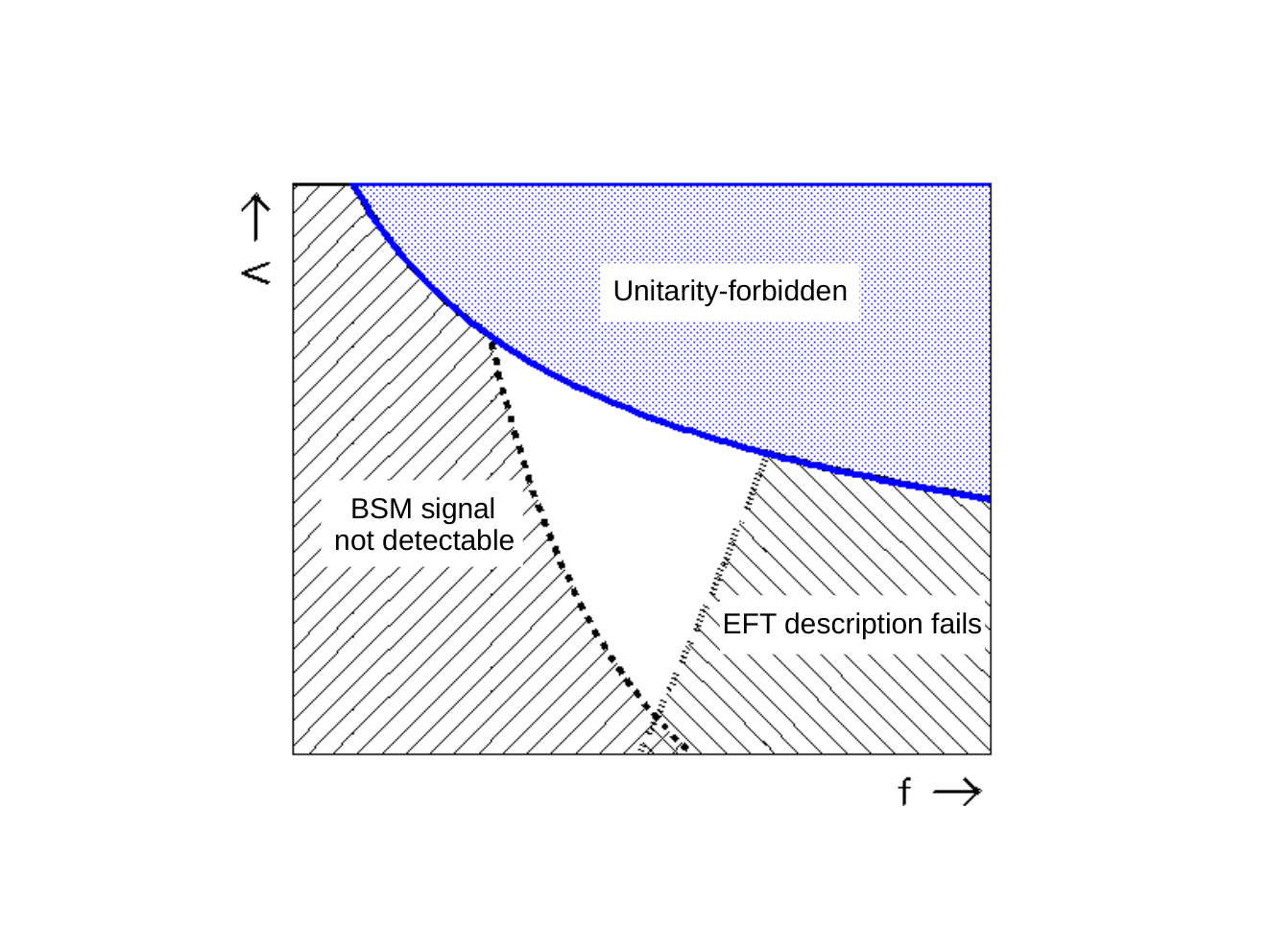
Thus, our preferred strategy for data analysis is as follows:
- 1.
From collected data measure a distribution (possibly in more than one dimension) that offers the highest sensitivity to the studied operator(s),
- 2.
If deviations from the SM are indeed observed 22 2 We do not discuss in this paper the bounds on the Wilson coefficients obtained from the data analysis when no statistically significant signal on new physics is observed. Such an analysis requires a separate discussion, although it will be also influenced by the results of this paper., fit particular values of based on EFT simulated templates in which the contribution from the region is taken into account according to Eq. (1.9) or using some more elaborated regularization methods,
- 3.
Fixing and to the fit values, recalculate the template so that the region is populated only by the SM contribution (Eq. (1.8)),
- 4.
Check statistical consistency between the original simulated template and the one based on Eq. (1.8),
- 5.
Physics conclusions from the obtained values can only be drawn if such consistency is found. In addition, stability of the result against different regularization methods provides a measure of uncertainty of the procedure - too much sensitivity to the region above means the procedure is destined to fail and so the physical conclusion is that data cannot be described with the studied operator.
2 Preliminary technicalities
The same-sign process probes a number of higher dimension operators. Among them are dimension-6 operators which modify only the Higgs-to-gauge coupling:
| (2.1) | |||
(the last one being CP-violating), dimension-6 operators which induce anomalous triple gauge couplings (aTGC):
| (2.2) | |||
(the last two of which are CP-violating), as well as dimension-8 operators which induce only anomalous quartic couplings (aQGC). In the above, is the Higgs doublet field, the covariant derivative is defined as
| (2.3) |
and the field strength tensors are
| (2.4) | |||
for gauge fields and of and , respectively.
Higgs and triple gauge couplings can be accessed experimentally via other processes, namely Higgs physics and diboson production which is most sensitive to aTGC. They are presently known to agree with the SM within a few per cent [13], which translates into stringent limits on the dimension-6 operators.
On the other hand, VBS processes are more suitable to constrain aQGC. The following dimension-8 operators contribute to the vertex:
| (2.5) | ||||
In the above, we have defined . Throughout this paper we follow the convention used in MadGraph [16] with dimension-8 operators included via public UFO files as far as the actual definitions of the field strength tensors and Wilson coefficients are concerned. Whenever results from the VBFNLO program [17] are used in this work, appropriate conversion factors are applied. For more details on the subject see Ref. [11].
The same-sign production has been already observed during Run I of the LHC [8, 9] and confirmed by a recent measurement of the CMS Collaboration at 13 TeV Run II [10]. Also, pioneering measurements of the [14] and [15] processes exist. They all place experimental limits on the relevant dimension-8 operators. However, most presently obtained limits involve unitarity violation within the measured kinematic range, leading to problems in physical interpretation and even comparison of the different analyses.
Our goal is to investigate the discovery potential at the High Luminosity LHC (HL-LHC) of the BSM physics effectively described by EFT “models” with single dimension-8 operators at a time, with proper attention paid to the regions of validity of such models, as described in Section 1.
3 Results of simulations
For the following analysis dedicated event samples of the process at 14 TeV were generated at LO using the MadGraph5_aMC@NLO v5.2.2.3 generator [16], with the appropriate UFO files containing additional vertices involving the desired dimension-8 operators. For each dimension-8 operator a sample of at least 500,000 events within a phase space consistent with a VBS-like topology (defined below) was generated. A preselected arbitrary value of the relevant coefficient (from now on, with ) was assumed at each generation; different values were obtained by applying weights to generated events, using the reweight command in MadGraph. The value =0 represents the Standard Model predictions for each study. The Pythia package v6.4.1.9 [18] was used for hadronization as well as initial and final state radiation processes. No detector was simulated. Cross sections at the output of MadGraph were multiplied by a factor 4 to account for all the lepton (electron and/or muon) combinations in the final state.
In this analysis, the Standard Model process is treated as the irreducible background, while signal is defined as the enhancement (which may be positive or negative in particular cases) of the event yield in the presence of a given dimension-8 operator relative to the Standard Model prediction. No reducible backgrounds were simulated, as they are known to be strongly detector dependent. For this reason, results presented here should be treated mainly as a demonstration of our strategy rather than as a precise determination of numerical values. For more realistic results this analysis should be repeated with full detector simulation for each of the LHC experiments separately.
The final analysis is performed by applying standard VBS-like event selection criteria, similar to those applied in data analyses carried by ATLAS and CMS. These were: 500 GeV, 2.5, 30 GeV, 5, 25 GeV, 2.5. As anticipated in Section 1, signal is calculated in two ways. First, using Eq. (1.8), where can vary in principle between and the appropriate unitarity limit for each chosen value of . The tail of the distribution is then assumed identical as in the Standard Model case. Second, using Eq. (1.9) which accounts for an additional BSM contribution coming from the region . The latter is estimated under the assumption that helicity amplitudes remain constant above this limit, as discussed in Section 1. For the case when is equal to the unitarity limit, this corresponds to unitarity saturation.
For each value of every dimension-8 operator, signal significance is assessed by studying the distributions of a large number of kinematic variables. We only considered one-dimensional distributions of single variables. Each distribution was divided into 10 bins, arranged so that the Standard Model prediction in each bin is never lower than 2 events. Overflows were always included in the respective highest bins. Ultimately, each distribution had the form of 10 numbers, that represent the expected event yields normalized to a total integrated luminosity of 3 ab-1, each calculated in three different versions: for the Standard Model case, from applying Eq. (1.8), and from applying Eq. (1.9) (here subscript runs over the bins). In this analysis, Eq. (1.9) was implemented by applying additional weights to events above in the original non-regularized samples generated by MadGraph. For the dimension-8 operators, this weight was equal to . The choice of the power in the exponent takes into account that the non-regularized total cross section for scattering grows less steeply around than its asymptotic behavior , which is valid in the limit . This follows from the observation that unitarity is first violated much before the cross section gets dominated by its term, as shown in the Appendix. The applied procedure is supposed to ensure that the total scattering cross section after regularization behaves like for , and so it approximates the principle of constant amplitude (Section 1), at least after some averaging over the individual helicity combinations. Examples of simulated distributions are shown in Fig. 2.
Signal significance expressed in standard deviations () is defined as the square root of a resulting from comparing the bin-by-bin event yields:
| (3.1) |
Lower observation limits on each operator are defined by the requirement of signal significance being above the 5 level. Small differences between the respective signal predictions obtained using Eqs. (1.8) and (1.9), as well as using other regularization techniques, will be manifest as slightly different observation limits and should be understood as the uncertainty margin arising from the unknown physics above , no longer described in terms of the EFT. Examples of signal significances as a function of are shown in Fig. 3 with dashed curves. Consistency of the EFT description is determined by requiring a small difference between the respective predictions from Eqs. (1.8) and (1.9). An additional is computed based on the comparison of the respective distributions of and :
| (3.2) |
In this analysis we allowed differences amounting to up to 2 in the most sensitive kinematic distribution. This difference as a function of is shown in Fig. 3 as dotted curves. These considerations consequently translate into effective upper limits on the value of for each operator.
For each dimension-8 operator we took the distribution that produced the highest among the considered variables. The most sensitive variables we found to be [19] for and , and [20] for the remaining operators (for some of them, would give almost identical results as , but usually this was not the case).
Unitarity limits were computed using the VBFNLO [17] calculator v1.3.0, after applying appropriate conversion factors to the input values of the Wilson coeeficients, so to make it suitable to the MadGraph 5 convention. We used the respective values from T-matrix diagonalization, considering both and channels, and taking always the lower value of the two. For the operators we consider here, unitarity limits are lower for than for except for (both positive and negative) and negative .


Assuming is equal to the respective unitarity bounds, the lower and upper limits for the values of for each dimension-8 operator, for positive and negative values, estimated for the HL-LHC with an integrated luminosity of 3 ab-1, are read out directly from graphs such as Fig. 3 and listed below in Table 1. These limits define the (continous) sets of testable EFT “models” based on the choice of single dimension-8 operators.
| Coeff. | Lower limit | Upper limit | Coeff. | Lower limit | Upper limit |
|---|---|---|---|---|---|
| (TeV-4) | (TeV-4) | (TeV-4) | (TeV-4) | ||
| 1.3 | 2.0 | 1.2 | 2.0 | ||
| 8.0 | 6.5 | 5.5 | 6.0 | ||
| 0.08 | 0.13 | 0.05 | 0.12 | ||
| 0.03 | 0.06 | 0.03 | 0.06 | ||
| 0.20 | 0.25 | 0.10 | 0.20 | ||
| 1.0 | 1.2 | 1.0 | 1.2 | ||
| 1.0 | 1.9 | 0.9 | 1.8 | ||
| 2.0 | 2.4 | 2.0 | 2.4 | ||
| 1.1 | 2.8 | 1.3 | 2.8 |
The fact that the obtained lower limits are more optimistic than those from several earlier studies (see, e.g., Ref. [21]) reflects our lack of detector simulation and reducible background treatment, but may be partly due to the use of the most sensitive kinematic variables. It must be stressed, nonetheless, that both these factors affect all lower and upper limits likewise, so their relative positions with respect to each other are unlikely to change much.
As can be seen, the ranges are rather narrow, but in most cases non-empty. Rather wide regions where BSM signal significance does not preclude consistent EFT description can be identified for and regardless of sign, as well as somewhat smaller regions for , and . Prospects for , and may depend on the accuracy of the high- tail modeling and a narrow window is also likely to open up unless measured signal turns out very close to its most conservative prediction. Only for positive values of , the resulting upper limit for consistent EFT description remains entirely below the lower limit for signal significance.
Allowing that the scale of new physics may be lower than the actual unitarity bound results in 2-dimensional limits in the plane. Usually this means further reduction of the allowed ranges for lower values and the resulting regions take the form of an irregular triangle. Respective results for all the dimension-8 operators are depicted in Figs. 4 and 5. It is interesting to note that in many cases this puts an effective lower limit on itself, in addition to the upper limit derived from the unitarity condition. In particular, the adopted criteria bound the value of to being above 2 TeV for the operators as well as for . The operators still allow a wider range of . Unfortunately, there is little we can learn from fitting , since signal observability requires very low values, for which the new physics could probably be detected directly.
It is interesting to plot the values of the couplings in Eq. (1.1) as a function of assuming i.e., , where is the dimensionality of the operator that defines the EFT “model”. In models with one BSM scale and one BSM coupling constant has the interpretation of the coupling constant [1]. The values of are to a good approximation independent of (see Fig. 6) and, being generally in the range (), reflect the approach to a strongly interacting regime in an underlying (unknown) UV complete theory. The EFT discovery regions depicted in Figs. 4 and 5 have further interesting implications for the couplings . For a fixed , the unitarity bound implies that , whereas the lower bound on that comes from the combination of the signal significance and EFT consistency criteria gives us . Thus, a given range corresponds to a range of values of the couplings , so that we could not only discover an indirect sign of BSM physics, but also learn something about the nature of the complete theory, whether it is strongly or weakly interacting. In particular, for the following operators: , , , and , only models with being close to the strong interaction limit will be experimentally testable, while a wider range of may be testable for , and .


4 Conclusions and outlook
In this paper we have analyzed the prospects for discovering physics beyond the SM at the HL-LHC in the EFT framework applied to the VBS amplitudes, in the process . We have introduced the concept of EFT “models” defined by the choice of higher dimension operators and values of the Wilson coefficients and analyzed “models” based on single dimension-8 operators at a time. We emphasize the role of the invariant mass whose distribution directly relates to the intrinsic range of validity of the EFT approach, , and the importance to tackle this issue correctly in data analysis in order to study the underlying BSM physics. While this is relatively simple (in principle) for final states where can be determined on an event-by-event basis, the value of is unfortunately not available in leptonic decays. We argue that usage of EFT “models” in the analysis of purely leptonic decay channels requires bounding the possible contribution from the region , no longer described by the “model”, and ensuring it does not significantly distort the measured distributions compared to what they would have looked from the region of EFT validity alone.
We propose a data analysis strategy to satisfy the above requirements and verify in what ranges of the relevant Wilson coefficients such strategy can be successfully applied in a future analysis of the HL-LHC data. We find that, with a possible exception of , all dimension-8 operators which affect the quartic coupling have regions where a 5 BSM signal can be observed at HL-LHC with 3 ab-1 of data, while data could be satisfactorily described using the EFT approach.
From such analysis it may be possible to learn something about the underlying UV completion of the full theory. Successful determination of a given value, using a procedure that respects the EFT restricted range of applicability, will put non-trivial bounds on the value of and consequently, the BSM coupling . These bounds are rather weak for , and operators, but potentially stronger for , , and . In particular, applicability of the EFT in terms of these operators already requires 2 TeV, while stringent upper limits arise from the unitarity condition. Because of relatively low sensitivity to and , it will unfortunately be hard to learn much about physics using the EFT approach with dimension-8 operators.
It must be stressed that in this analysis we have only considered single dimension-8 operators at a time. Allowing non-zero values of more than one at a time provides much more felixibility as far as the value of is concerned, especially for those operators whose individual unitarity limits are driven by helicity combinations which contribute little to the total cross section. Consequently, regions of BSM observability and EFT consistency can only be larger than what we found here. Study of VBS processes in the EFT language can be the right way to look for new physics and should gain special attention in case the LHC fails to observe new physics states directly.
Consideration of other VBS processes and decay channels may significantly improve the situation. In particular, the semileptonic decays, where one decays leptonically and the other into hadrons, have never been studied in VBS analyses because of their more complicated jet combinatorics and consequently much higher background. Progress in the implementation of -jet tagging techniques based on jet substructure algorithms may render these channels interesting again. However, they are presently faced with two other experimental challenges. One is the precision of the determination which relies on the missing- measurement resolution. The other one is poor control over the sign over the hadronic . The advantages would be substantial. If can be reconstructed with reasonable accuracy, it is straightforward to fit and to the measured distribution in an EFT-consistent way even for arbitrarily large . Existence of a high- tail above is then not a problem, but a bonus, as it may give us additional hints about the BSM physics. Finally, because of the invariant mass issue, the scattering channel, despite its lowest cross section, may ultimately prove to be the process from which we can learn the most about BSM in case the LHC fails to discover new physics directly.
Acknowledgments
The work of SP is partially supported by the National Science Centre, Poland, under research grants DEC-2014/15/B/ST2/02157, DEC-2015/18/M/ST2/00054 and DEC-2016/23/G/ST2/04301, and that of JK by the Polish National Science Center HARMONIA project under contract UMO-2015/18/M/ST2/00518 (2016-2019). JR is supported in part by the National Science Center, Poland, under research grant DEC2015/19/B/ST2/02848. ST is supported by Fermi Research Alliance, LLC under Contract No. De-AC02-07CH11359 with the United States Department of Energy.
Appendix A Unitarity bounds
The purpose of this section is to give an overview of the behavior of individual helicity amplitudes as a function of energy and their contributions to the total unpolarized cross section, with special attention paid to the partial wave unitarity constraints, in the SM and in its extensions to the EFT “models” discussed in this paper. We shall illustrate the main points using the operators and . The choice is determined by the requirement that the bounds for which we present below are stronger than for (often used in our analyses). The qualitative picture remains the same for the other operators as well. Analytical computations have been partially performed using a Mathematica code. All cross sections are computed with a cut in the forward and backward scattering regions. Similarly, a cut is applied for partial amplitudes, hence for determination.
We begin by choosing a set of independent helicity amplitudes for scattering. Altogether, there are 81 helicity amplitudes for this process but and discrete symmetries and the fact that the state has a symmetric wave function (Bose statistics) impose many relations between them and leave only 13 amplitudes as an independent set. We choose them as follows:
| (A.1) |
Here , and denote the right-handed, left-handed and longitudinal polarizations, respectively; the first two symbols define the initial state and the last two symbols define the final state. These amplitudes contribute to the total cross section with multiplicities
respectively, due to symmetry relations between all the 81 amplitudes. In the SM their energy dependence is at most flat but their magnitude can differ by orders of magnitude (see Table 2 for their energy dependence and the contribution of the corresponding polarized cross sections to the total unpolarized cross section at 1 TeV). The unpolarized cross section (decreasing like ) is saturated by just four of them, taking into account the corresponding multiplicities (see Fig. 7).
The next thing of interest for us is the scattering energy at which partial wave unitarity is violated by different helicity amplitudes for the two operators considered in this section, according to the tree level criterion . This is shown in Table 3 for the operator (positive ) and in Table 4 for (negative ), as a function of the values of . We see that partial wave unitarity is first violated in the amplitude for the first operator and in for the second one. Unitarity is violated at vastly different energies for different helicity amplitudes, depending on the operator considered. Some of them remain constant with energy, in particular some of those that saturate the SM total cross section. The leading energy dependences of the amplitudes and the contributions of polarized cross sections to the total unpolarized cross section at the lowest where the first helicity amplitude violates partial wave unitarity are shown in Tables 5 and 6, respectively. One sees that for , the cross section (related to the amplitude which violates unitarity first) gives about 65% of the total cross sections, independently of the value of , for the corresponding values of minimal . For , it is the cross section, closely followed by , with an about 80% combined contribution to the total unpolarized cross section, independently of the value of , for the corresponding values of minimal . The rest of the unpolarized cross sections at the minimal come (for both operators) from the helicity amplitudes that saturate the cross section in the SM, which either remain constant with energy (although weakly dependent on the value of ) or violate perturbative partial unitarity at a higher energy.
Unitarity bounds calculated from T-matrix diagonalization are virtually identical to those for the amplitude that determines the minimal for , while for they are about 15% lower.
Some examples of the energy dependence of the cross sections for both operators are shown in the following figures: for the total unpolarized cross sections with in Fig. 8, for polarized cross sections with in Fig. 10, for unpolarized with in Fig. 9, and for polarized with in Fig. 11. We observe that both operators show several similar interesting features. Below the partial wave unitarity minimal bounds , sizable deviations from the SM predictions occur only for small energy intervals close to those bounds. This is the region where the quadratic term in Eq. (1.3) begins to dominate BSM effects (see Figs. 8 and 9). The contribution of the interference term at this point generally depends on which helicity combinations get affected by a given operator and how much they contribute to the total cross section in the SM. Interference is visible for , , , , , , , and negligible for and . The energy dependence of the unpolarized cross sections around the values of the minimal is moreover somewhat weakened by the contribution from the helicity amplitudes that have not reached the unitarity limit.
References
- [1] G. F. Giudice, C. Grojean, A. Pomarol and R. Rattazzi, JHEP 0706 (2007) 045, doi:10.1088/1126-6708/2007/06/045 [hep-ph/0703164].
- [2] A. Biekˆtter, A. Knochel, M. Krämer, D. Liu and F. Riva, Phys. Rev. D 91 (2015) 055029, doi:10.1103/PhysRevD.91.055029 [arXiv:1406.7320 [hep-ph]].
- [3] D. Liu, A. Pomarol, R. Rattazzi and F. Riva, JHEP 1611 (2016) 141, doi:10.1007/JHEP11(2016)141 [arXiv:1603.03064 [hep-ph]].
- [4] R. Contino, A. Falkowski, F. Goertz, C. Grojean and F. Riva, JHEP 1607 (2016) 144, doi:10.1007/JHEP07(2016)144 [arXiv:1604.06444 [hep-ph]].
- [5] A. Azatov, R. Contino, C. S. Machado and F. Riva, Phys. Rev. D 95 (2017) no.6, 065014, doi:10.1103/PhysRevD.95.065014 [arXiv:1607.05236 [hep-ph]].
- [6] R. Franceschini, G. Panico, A. Pomarol, F. Riva and A. Wulzer, arXiv:1712.01310 [hep-ph].
- [7] A. Falkowski, M. Gonzalez-Alonso, A. Greljo, D. Marzocca and M. Son, JHEP 1702 (2017) 115, doi:10.1007/JHEP02(2017)115 [arXiv:1609.06312 [hep-ph]].
- [8] G. Aad et al. [ATLAS Collaboration], Phys. Rev. Lett. 113 (2014) no.14, 141803, doi:10.1103/PhysRevLett.113.141803 [arXiv:1405.6241 [hep-ex]].
- [9] V. Khachatryan et al. [CMS Collaboration], Phys. Rev. Lett. 114 (2015) no.5, 051801, doi:10.1103/PhysRevLett.114.051801 [arXiv:1410.6315 [hep-ex]]. M. Aaboud et al. [ATLAS Collaboration], Phys. Rev. D 96 (2017) no.1, 012007, doi:10.1103/PhysRevD.96.012007 [arXiv:1611.02428 [hep-ex]].
- [10] A. M. Sirunyan et al. [CMS Collaboration], Phys. Rev. Lett. 120 (2018), 081801, doi:10.1103/PhysRevLett.120.081801 [arXiv:1709.05822 [hep-ex]].
- [11] C. Degrande et al., arXiv:1309.7890 [hep-ph].
- [12] O.J.P. Éboli and M.C. Gonzalez-Garcia, Phys. Rev. D 93 (2016) no.9, 093013, doi:10.1103/PhysRevD.93.093013 [arXiv:1604.03555 [hep-ph]].
- [13] For a combined analysis of LEP and Run I LHC data, see e.g. A. Butter, O.J.P. Éboli, J. Gonzalez-Fraile, M.C. Gonzalez-Garcia, T. Plehn and M. Rauch, JHEP 1607 (2016) 152, doi:10.1007/JHEP07(2016)152 [arXiv:1604.03105 [hep-ph]].
- [14] G. Aad et al. [ATLAS Collaboration], Phys. Rev. D 93 (2016) no.9, 092004, doi:10.1103/PhysRevD.93.092004 [arXiv:1603.02151 [hep-ex]].
- [15] A. M. Sirunyan et al. [CMS Collaboration], Phys. Lett. B 774 (2017) 682, doi:10.1016/j.physletb.2017.10.020 [arXiv:1708.02812 [hep-ex]].
- [16] J. Alwall et al., JHEP 07 (2014) 079, doi:10.1007/JHEP07(2014)079 [arXiv:1405.0301 [hep-ph]].
- [17] K. Arnold et al., Comput. Phys. Commun. 180 (2009) 1661, doi:10.1016/j.cpc.2009.03.006 [arXiv:0811.4559 [hep-ph]]; J. Baglio et al. arXiv:1107.4038 [hep-ph], arXiv:1404.3940 [hep-ph].
- [18] T. Sjostrand, S. Mrenna, P. Skands, JHEP 0605 (2016) 026, doi:10.1088/1126-6708/2006/05/026 [arXiv:hep-ph/0603175].
- [19] K. Doroba et al., Phys. Rev. D 86 (2012) no.3, 036011, doi:10.1103/PhysRevD.86.036011 [arXiv:1201.2768 [hep-ph]].
- [20] S. Todt, Ph.D. Thesis CERN-THESIS-2015-018, TU Dresden, 2015.
- [21] C. Degrande et al., arXiv:1309.7452 [physics.comp-ph].