Outlier Detection for Robust Multi-dimensional Scaling
Abstract
Multi-dimensional scaling (MDS) plays a central role in data-exploration, dimensionality reduction and visualization. State-of-the-art MDS algorithms are not robust to outliers, yielding significant errors in the embedding even when only a handful of outliers are present. In this paper, we introduce a technique to detect and filter outliers based on geometric reasoning. We test the validity of triangles formed by three points, and mark a triangle as broken if its triangle inequality does not hold. The premise of our work is that unlike inliers, outlier distances tend to break many triangles. Our method is tested and its performance is evaluated on various datasets and distributions of outliers. We demonstrate that for a reasonable amount of outliers, e.g., under , our method is effective, and leads to a high embedding quality.
I Introduction
Multi-dimensional Scaling (MDS) is a fundamental problem in data analysis and information visualization. MDS takes as input a distance matrix , containing all pairs of distances between elements , and embeds the elements in dimensional space such that the pairwise distances are preserved as much as possible by in the embedded space. When the distance data is outlier-free, state-of-the-art methods (e.g., SMACOF) provide satisfactory solutions [1, 2]. These solutions are based on an optimization of the so-called stress function, which is a sum of squared errors between the dissimilarities and their corresponding embedding inter-vector distances:
In many real-world scenarios, input distances may be noisy or contain outliers, due to malicious acts, system faults, or erroneous measures. Many MDS techniques deal with noisy data [3, 4], but little attention has been given to outliers [5, 6, 7]. We refer to outliers as opposed to noise, as distances that are significantly different than their corresponding true values.
Developing a robust MDS is challenging since even a small portion of outliers can lead to significant errors. This sensitivity of MDS to outliers is demonstrated in Figure 1, where only two pairwise distances (out of 435 pairs) are erroneous (colored in red in (a)), cause a strong distortion in the embedding (b). To highlight the embedding errors, we draw lines connecting between the ground truth positions and the embedded positions.
In this paper, we introduce a robust MDS technique, which detects and removes outliers from the data and hence provides a better embedding.
Our approach is based on geometric reasoning with which the outliers can be identified by analyzing the given input distances. This approach follows the well-known idiom ”prevention is better than a cure”. That is, instead of recovering from the damage that the outliers cause to the MDS optimization, we prevent them in the first place, by detecting and filtering them out.
We treat the distances as a complete graph of edges. Each edge is associated with its corresponding distance and forms triangles with the rest of the nodes. The premise of our work is that an outlier distance tends to break many triangles. We refer to a triangle as broken if its triangle inequality does not hold. As we shall show, while inlier edges participate in a rather small number of broken triangles, outlier edges participate in many. This allows us to set a conservative threshold and classify the edges and their associated distances as inliers and outliers (See Figure 2).
Generally speaking, MDS is an overdetermined problem since the distance matrix contains many more distances than necessary to solve the problem correctly. Hence, the idea is to detect distances that are suspected to be outliers and remove them before applying the MDS. In the following, we denote and refer to our robust MDS method with TMDS. As we shall show, our technique succeeds in detecting and removing most of the outliers without any parameters, while incurring a rather small number of false positives, to facilitate a more accurate embedding. We tested, analyzed and evaluated our method on a large number of datasets with varying portions of outliers from various distributions.
II Background
MDS was originally used and developed in the field of Psychology, as a means to visualize perceptual relations among objects[8, 9]. Nowadays, MDS is used in a wide variety of fields, such as marketing [10], and graph embedding [11]. Most notably, MDS plays a central role in data exploration [12, 13, 14], and computer graphics applications like texture mapping [15], shape classification and retrieval [16, 17, 18] and more.
Several methods were suggested to handle outliers in the data (e.g., [5, 7]). Using Sammon weighting [19] leads to the following stress function:
This objective function can effectively be considered as robust to elongated distances since it decreases the weights of long distances. We differentiate between two types of outliers: larger and shorter outliers (colored in blue and red, respectively, in Figures 3 and 4), since their characteristics and effects are different and may thus require different treatments. In (a) we show 2D data elements, where the outliers are marked in red and blue. In (b) we show their positions recovered by applying a state-of-the-art MDS (i.e., SMACOF) and in (c) the results of Sammon method [19]. As can be observed, Sammon method can deal well with elongated distances, by assigning them with low weights. However, shortened distances are not dealt with well, as they are assigned larger weights which lead to a distorted embedding.
The most related work to ours is the method presented by Forero and Giannakis [6], hereafter referred to as FG12. They use an objective function that aims to find an embedding and an outliers matrix that minimize the following:
where regulates the number of non-zero values in that represent outliers.
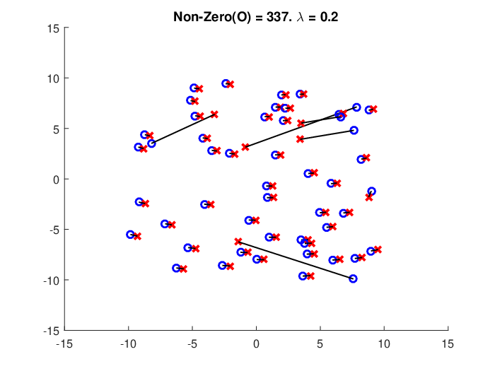
Setting the size of to control the sparsity of is not easy. If is too big, too few outliers are detected; if it is too small, too many edges are treated as outliers. As we shall show, close values of can lead to different results. This phenomenon is shown in Figure 5 (a-c). Thus, careful tuning of is required to achieve good results. This is an overly complex process, since, as well shall show, the algorithm is also sensitive to the initial guess.
Note that has unknown variables and has variables. This amounts to a considerable increase in the number of parameters, and hence it is significantly harder to optimize FG12 compared to SMACOF. This is evident in Figure 5 where we show (d-f) that with the same applied to the same dataset, but with different initial guesses. As shown, the three initial guesses yield a different number of edges that are considered as outliers. This behavior of the FG12 method can also be observed in Figure 6. Note that for the yellow curve, is the value that detects the correct number of outliers. However, for the same value of the blue plot detects most of the edges as outliers. This highlights the sensitivity of the FG12 method and emphasizes that we cannot set the value of even when we have a good estimation of the number of outliers in the system.

III Detecting outliers
Our technique estimates the likelihood of each distance to be an outlier. We treat the distances as a complete graph of edges connecting the vertices. Each edge is associated with its corresponding distance and forms triangles with the rest of the elements. The key idea is that inlier edges participate in a rather small number of broken triangles, while outlier edges participate in many. As we shall see, by analyzing the histogram of broken triangles, we can set a conservative threshold and classify the edges and their associated distances as inliers and outliers. See Figure 2.
Let represent the pairwise distances among graph vertices. In the presence of outliers, some of the edges do not represent a correct Euclidean relation. In particular, an erroneous edge length tends to break a triangle formed by the edge and its two endpoint vertices, and a third vertex from among the rest of the vertices. Recall that here, a broken triangle is one for which the triangle inequality does not apply.
We can easily identify all the broken triangles by traversing all triangles in the graph. For any triangle with edges of length where , we test: We then count for each of the edges in the graph, the number of broken triangles it participates in. This yields a histogram , where counts the number of edges that participate in broken triangles. Figure 7 depicts such a typical histogram. As can be observed, most of the edges participate in a small number of broken triangles. The long tail of the histogram is associated with outliers.
It should be noted that an outlier edge does not necessarily break all its triangles, but in large numbers it stands out, and as we shall see, is likely to be detected.
We wish to determine a threshold to classify the outlier. That is, an edge which participates in more than broken triangles is classified as an ourlier. The threshold cannot be set to accurately classify the inlier/outlier edges. Instead, we propose a simple way to determine this threshold by analyzing the histogram . We set to be the smallest value that satisfies the following two requirements:
- 1.
- 2.
The first requirement assures that most of the edges are not considered as outliers. This assumption holds in most cases, but can be adjusted according to the problem setting. The second requirement corresponds to the observation that outlier edges tend to form a high bin along the tail of the histogram (Figure 7). This simple heuristic performs well empirically (see Section IV).
After the threshold is selected, we can remove the associated distances from the data, and use the remaining distances to compute an embedding using MDS. A high-level pseudo code of TMDS is described in Algorithm 1.
IV Analysis
IV-A Algorithm complexity
Testing all the triangles to identify the broken ones, amounts to a time complexity of , an order of magnitude larger than that of SMACOF (). To avoid increasing the total time complexity of the MDS method, we can subsample triangles and build the histogram based only on them. We can use uniform sampling, where, for every edge , we sample a constant number of points to form a constant number of triangles. As can be observed in Figure 8, testing too few triangles, may impair the detection rate. It can be seen that 45 triangles per edge are enough to detect most of the outliers, and that it scales well with N. Empirically, we observed that sampling twice as many triangles as the expected number of outliers is an effective rule-of-thumb. In practice, for TMDS without any sub-sampling takes only seconds using a non-optimized implementation in Matlab, while computing the embedding itself using SMACOF takes seconds. This suggests that the filtering step does not incur significant overhead. See Table I.
| N | SMACOF | TMDS | FG12 |
|---|---|---|---|
| 150 | 2 | 4.84 | 15.9 |
| 300 | 3.5 | 9.35 | 59.4 |
| 450 | 5.5 | 19.6 | 105.5 |
| 600 | 8.9 | 32.2 | 207.8 |
| 750 | 13.5 | 46.9 | 309.4 |
| 900 | 14.8 | 59.9 | 491.4 |

IV-B Evaluation
To evaluate TMDS, we use synthesized data of various magnitudes, dimensions, and portions of outliers. We measure the precision-recall performance of detecting the outliers, and the quality of the embedding with and without our outlier filtering. More precisely, we synthesize ground-truth data by randomly sampling points in a dimensional hypercube, and compute the pairwise distances between them. We randomly pick elements and replace them with a random element from the distance matrix.
Qualitative evaluation. We use Shepard Diagrams to visually display the classification of data elements as either outliers or inliers. In the diagram in Figure 9, each point represents a distance. The X-axis represents the input distances and the Y-axis represents the distance in the embedding result. Points on the main diagonal are inliers representing the distances that are correctly preserved in the embedding. The red circles represent the distances that TMDS detects as outliers. The blue off-diagonal points are the false negatives, and the red dots on the diagonal are false positive distances. The number of false positives and negatives increases as the number of outliers increases.

Quantitative evaluation. We employ two models to quantitatively evaluate TMDS. In the first, we select outliers at random, while in the second all edges are distorted by a log-normal distribution.
First, we measure the accuracy of outlier detection using precision-recall. Each distance is classified as either inlier or outlier, and the detection can thus be regarded as a retrieval process, where precision is the fraction of retrieved outliers that are true positives, and recall is the fraction of true positives that are detected. As can be observed in Figure 10, our precision and recall are high, where the first moderately decreases with the number of outliers and the latter increases. The precision is larger than , which implies that a non-negligible portion of the filtered distances are false positives. However, the excess of filtering is not destructive since MDS is an over-determined problem. Yet, at some point, filtering too many distances impairs the embedding, as will be demonstrated in a separate experiment below.

The detection probability. Figure 11 shows the probability of an outlier to be detected as a function of its error magnitude, which is measured by the ratio between the actual distance and the true distance . As can be observed, edges that are strongly deformed (either squeezed or enlarged) are likely to be detected. This holds also for higher dimensions.
Embedding evaluation. To obtain insight about the embedding performance of points , we used the following score:
Then, we take the average of as the score for the embedding. This scoring treats shrinkage and enlargements equally, where a low score implies a better embedding. The results of the evaluation are displayed in Figure 12. The plot shows that when the portion of outliers is less than , our pre-filtering performs better than applying SMACOF MDS directly. A larger amount of outliers causes TMDS to filter out too many inliers and impairs the embedding.
Log-normal distribution. We generated synthetic data that mimics realistic data characteristics, by sampling data points uniformly in a -dimensional hypercube, and forming the respective distance matrix . We distorted the distances using factors of log-normal distribution. That is, every distance is multiplied by a factor sampled from a log-normal distribution, where the log-normal mean is 1. Note that these distorted distances include both noise and outliers. The results of those simulations with different log standard deviation are presented in Figure 13. Note that for larger values, which signify larger errors, the effectiveness of TMDS is more significant.
Non-uniform Distributions. We further evaluated TMDS on non-uniform structured data. The embedding of data sets with clear structures are shown in Figure 14. As we shall discuss below, one of the limitations of TMDS is handling straight lines. This is evident in Figure 14, where our embedding is imperfect (b), albeit better than without filtering (a). In (c-d), the structured data is numerically easier for filtering. As demonstrated, the accuracy of the embedding of the data with outliers is high.


IV-C Limitations
As described, our algorithm consists of two parts - building the histogram of broken triangles and setting the threshold. Each part has it own limitations. The analysis of the histogram assumes that outlier edges break many triangles, while inliers do not. This assumption may not hold when a large number of triangles are broken also by inlier distances. This may happen when , but due to numerical issues, , for example, when many points reside along straight lines. Setting the threshold is merely a heuristic that may fail when there are too many outliers, or too few that have a special distribution that confuses the heuristics and causes half of the data to be considered as outliers.
V Experiments
A Matlab implementation is available at goo.gl/399buj.
In the previous sections, we have tested and evaluated our method (TMDS) using synthetic data for which we have the ground truth distances. We have shown that the MDS technique of Forero and Giannakis [6] is sensitive to the initial guess and its performance is dependent on a user-selected parameter. In the following, we evaluate our method on data for which the ground truth is not available. To evaluate the performance, we compare TMDS with a SMACOF implementation of MDS using numerous common measures that assume ground truth labels, but not distances. The labels are used for evaluation only. First, we test TMDS on two real datasets available on the Web, for which the ground truth distances are available. Next, we evaluate TMDS on three datasets for which ground truth distances are unavailable, but classes labels exist.
SGB128 dataset This dataset consists of the locations of 128 cities in North America [20]. We compute the distances among the cities, and introduce outliers. Figure 15 shows the ground-truth locations, the embedding obtained by SMACOF on the outlier data and the result of SMACOF after applying our filtering technique. As can be seen, applying the filtering prior to computing the embedding yields a significant improvement.


Protein dataset This dataset consists of a proximity matrix derived from the structural comparison of 213 protein sequences [21, 22].These dissimilarity values do not form a metric. Each of these proteins is associated with one of four classes: hemoglobin-α (HA), hemoglobin-β (HB), myoglobin (M) and heterogeneous globins (G). We embed the dissimilarities using SMACOF with and without our filtering. We then perform -means clustering and evaluate the clusters with respect to the ground-truth classes. The results are shown in Figure 16. The clustering results are evaluated using four common measures: ARI, RI and MOC. As can be seen, TMDS outperforms a direct application of SMACOF by all the measures.
VI Graphical Datasets
In the following, we conduct experiments to show the effectiveness of our robust MDS for visualization of graphical elements. Specifically, we use three datasets, one of 2D shapes taken from the MPEG7 dataset [23] and 1070db [24] shape dataset, one of motion data (CMU Motion Capture Database mocap.cs.cmu.edu) and one of 3D shapes [25]. For each of the sets we use an appropriate distance measure to generate an all-pairs distance matrix, and then create a map by embedding the elements using SMACOF MDS and our robust MDS. More specifically, we use inner distance to measure distances between 2D shapes, LMA-features [26] for measuring distances between sequences, and SHED [27] to measure the distances among 3D shapes.
We evaluate the embedding qualitatively and quantitatively. Since the ground truth is unavailable, we use the known classes for the evaluation. We expect a good embedding to separate the classes into tight clusters, and specifically avoid intersections among them. Qualitatively, this can be observed in the three side-by-side comparisons of the SMACOF vs. TMDS embedding in Figures 17, 18, 20, 22, and 21. To measure it quantitatively, we use two common measures, namely Silhouette Index [28] and Calinski Harabasz [29], which analyze how well the different classes are separated from each other. We also use common measures to analyze how well a clustering technique succeeds in clustering the data. We apply K-means and measure its success using AMI[30], NMI [31], and Completeness and Homogeneity measures [32]. As can be noted in Table II, our TMDS method outperforms SMACOF in all of these measures.


The dissimilarity measures we use in all the experiments are not a metric and thus the meaning of outliers should be understood accordingly. The removal of outliers in such a context merely enhances the distances to better conform with a metric. Nevertheless, as can be clearly seen, in all cases, TMDS enhances the maps and provides a better separation of the classes. Still, as can be observed in Figures 20, 21 and 22, the embedded results are not necessarily perfect, in the sense that there are some elements that are not embedded close enough to the rest of the elements in their respective classes. Note that for completeness, we add results obtained with the method of Forero and Giannakis [6], for which we set .


| Motion Data | MPEG7 | 3D Mesh | ||||
|---|---|---|---|---|---|---|
| Scoring | SMACOF | TMDS | SMACOF | TMDS | SMACOF | TMDS |
| Silhouette | 0.282 | 0.321 | 0.38 | 0.48 | 0.39 | 0.49 |
| Calinski Harabaz | 167.2 | 218.9 | 60.54 | 90.5 | 50.7 | 59.0 |
| AMI | 0.64 | 0.66 | 0.78 | 0.85 | 0.72 | 0.79 |
| Completeness | 0.65 | 0.68 | 0.79 | 0.86 | 0.80 | 0.83 |
| Homogeneity | 0.64 | 0.67 | 0.82 | 0.87 | 0.76 | 0.82 |
| NMI | 0.65 | 0.674 | 0.81 | 0.86 | 0.78 | 0.82 |
VII Distribution of distances

In this section, we seek to analyze the probability that a triangle is broken by an erroneous edge, assuming that errors have the same distribution as distances. Thus, given a triangle formed by in a -dimensional unit hypercube, we should learn the distribution of distances of triangle edges to facilitate the estimation of the probability that an erroneous edge breaks the triangle inequality.
We begin by analyzing the distribution of edge lengths. Let be two points in a -dimensional unit hypercube, uniformly randomly sampled.
The distance has normal distribution with mean and variance of and , respectively, and the approximation gets better as increases. The proof is provided in [33].
Hereafter, we denote and .
We empirically calculated - the covariance between and , for several dimensions, and found that it has a constant value of . This allows us to approximate the mean and variance for and , assuming that their distributions are normal:
These normal distributions are displayed in Figure 23 for dimensions , and . As can be noted, the accuracy of the approximations increases for higher dimensions.
Given the above distributions, we are now ready to estimate the probability of a triangle to break by an erroneous edge.
Theorem 1.
Let be three points uniformly randomly and independently sampled in a -dimensional unit hypercube. Given the above distance distributions, and let the edge be an outlier distance, the probability that the triangle is broken is
where stands for standard normal cumulative distribution function.
Proof.
It was shown above that
where stands for normal distribution.
Assuming that and , as well as and are independent, a triangle breaks if one of the following inequalities is satisfied:
Then, the probabilities for these independent cases are:
Thus, the probability for a triangle to break due to an outlier edge is simply their sum:
∎
Note that the assumption that an outlier behaves similarly to a common distance (i.e., same distributions) makes its detection harder.Nevertheless, as we showed above, an outlier breaks a large number of triangles. For example, assuming that triangles are independent, with , of the triangles that are associated with an outlier edge are broken. This number is validated by our empirical evaluations above. Also, note that is a function of , thus as the dimension increases, also increases, and the probability above decreases.
VIII Conclusions
We presented a technique to filter distances prior to applying MDS, so that it is more robust to outliers. The technique analyzes the triangles formed by three points and their pairwise distances, and associates distances to broken triangles. Not every outlier is associated with a broken triangle, and an edge associated with a broken triangle is not necessarily an outlier. Thus, it is expected to produce both false positives and false negatives. However, as we showed, as long as the portion of outlier edges is reasonable, i.e., , the false positives are non-destructive, and the quality of the embedding is high. Most notably, when the number of outliers is particularly small, as in reasonable real-world scenarios, the accuracy of our technique is particularly high and the improvement over a direct MDS is significant. We also showed that our technique is useful to distill the data before applying MDS, even when there are no significant outliers.
In our work, we focused on Euclidean metric, however, the technique can also be applied to other metrics. For example, in psychology and marketing it is common to use the family of Minkowsky distances [34, 35]:
As long as , our method applies.
Beyond the generalization to other metrics, our technique is applicable to general embedding, and not restricted to a specific stress function or MDS algorithm. As long as the embedding method does not require a full dissimilarity matrix, our method is viable.
We would like to stress that our method has no parameters. The threshold uses the value of , which is parameter-free. However, one can define with a parameter that reflects the expected number of outliers, to refine the accuracy of the method, i.e., to produce less false-positives.
References
- [1] J. De Leeuw, “Convergence of the majorization method for multidimensional scaling,” Journal of classification, vol. 5, no. 2, pp. 163–180, 1988.
- [2] J. d. Leeuw and P. Mair, “Multidimensional scaling using majorization: Smacof in r,” 2008.
- [3] V. De Silva and J. B. Tenenbaum, “Sparse multidimensional scaling using landmark points,” Technical report, Stanford University, Tech. Rep., 2004.
- [4] F. K. Chan and H.-C. So, “Efficient weighted multidimensional scaling for wireless sensor network localization,” IEEE Transactions on Signal Processing, vol. 57, no. 11, pp. 4548–4553, 2009.
- [5] I. Spence and S. Lewandowsky, “Robust multidimensional scaling,” Psychometrika, vol. 54, no. 3, pp. 501–513, 1989.
- [6] P. A. Forero and G. B. Giannakis, “Sparsity-exploiting robust multidimensional scaling,” IEEE Transactions on Signal Processing, vol. 60, no. 8, pp. 4118–4134, 2012.
- [7] L. Cayton and S. Dasgupta, “Robust euclidean embedding,” in Proceedings of the 23rd international conference on machine learning. ACM, 2006, pp. 169–176.
- [8] J. B. Kruskal, “Nonmetric multidimensional scaling: a numerical method,” pp. 115–129, 1964.
- [9] R. N. Shepard, “The analysis of proximities: multidimensional scaling with an unknown distance function. i.” pp. 125–140, 1962.
- [10] L. A. Neidell, “The use of nonmetric multidimensional scaling in marketing analysis,” pp. 37–43, 1969.
- [11] R. N. Shepard, “Multidimensional scaling, tree-fitting, and clustering,” Science, vol. 210, no. 4468, pp. 390–398, 1980.
- [12] I. Borg and P. J. Groenen, Modern multidimensional scaling: Theory and applications. Springer Science & Business Media, 2005.
- [13] A. Buja, D. F. Swayne, M. L. Littman, N. Dean, H. Hofmann, and L. Chen, “Data visualization with multidimensional scaling,” Journal of Computational and Graphical Statistics, vol. 17, no. 2, pp. 444–472, 2008.
- [14] A. Buja and D. F. Swayne, “Visualization methodology for multidimensional scaling,” Journal of Classification, vol. 19, no. 1, pp. 7–43, 2002.
- [15] G. Zigelman, R. Kimmel, and N. Kiryati, “Texture mapping using surface flattening via multidimensional scaling,” IEEE Transactions on Visualization and Computer Graphics, vol. 8, no. 2, pp. 198–207, 2002.
- [16] Z. Chen and K. Tang, “3d shape classification based on spectral function and mds mapping,” Journal of Computing and Information Science in Engineering, vol. 10, no. 1, p. 011004, 2010.
- [17] D. Pickup, X. Sun, P. L. Rosin, R. Martin, Z. Cheng, Z. Lian, M. Aono, A. B. Hamza, A. Bronstein, M. Bronstein et al., “Shrec’14 track: Shape retrieval of non-rigid 3d human models,” Proc. 3DOR, vol. 4, no. 7, p. 8, 2014.
- [18] Y. Li, H. Su, C. R. Qi, N. Fish, D. Cohen-Or, and L. J. Guibas, “Joint embeddings of shapes and images via cnn image purification,” ACM Trans. Graph., vol. 34, no. 6, pp. 234:1–234:12, Oct. 2015. [Online]. Available: http://doi.acm.org/10.1145/2816795.2818071
- [19] J. W. Sammon, “A nonlinear mapping for data structure analysis,” IEEE Transactions on computers, vol. 18, no. 5, pp. 401–409, 1969.
- [20] J. Burkardt, CITIES - City Distance Datasets, 2011.
- [21] T. Denœux and M.-H. Masson, “Evclus: evidential clustering of proximity data,” IEEE Transactions on Systems, Man, and Cybernetics, Part B (Cybernetics), vol. 34, no. 1, pp. 95–109, 2004.
- [22] T. Graepel, R. Herbrich, P. Bollmann-Sdorra, and K. Obermayer, “Classification on pairwise proximity data,” Advances in neural information processing systems, pp. 438–444, 1999.
- [23] H. Ling and D. W. Jacobs, “Using the inner-distance for classification of articulated shapes,” in Computer Vision and Pattern Recognition, 2005. CVPR 2005. IEEE Computer Society Conference on, vol. 2. IEEE, 2005, pp. 719–726.
- [24] Brown-University, 1070 Binary Shape Databases, http://vision.lems.brown.edu/content/available-software-and-databases,, 2005.
- [25] X. Chen, A. Golovinskiy, and T. Funkhouser, “A benchmark for 3D mesh segmentation,” ACM Transactions on Graphics, vol. 28, no. 3, 2009.
- [26] A. Aristidou, P. Charalambous, and Y. Chrysanthou, “Emotion analysis and classification: Understanding the performers emotions using the LMA entities,” Computer Graphics Forum, vol. 34, no. 6, p. 262–276, September 2015.
- [27] Y. Kleiman, O. van Kaick, O. Sorkine-Hornung, and D. Cohen-Or, “Shed: shape edit distance for fine-grained shape similarity,” ACM Transactions on Graphics (TOG), vol. 34, no. 6, p. 235, 2015.
- [28] P. J. Rousseeuw, “Silhouettes: a graphical aid to the interpretation and validation of cluster analysis,” Journal of computational and applied mathematics, vol. 20, pp. 53–65, 1987.
- [29] T. Caliński and J. Harabasz, “A dendrite method for cluster analysis,” Communications in Statistics-theory and Methods, vol. 3, no. 1, pp. 1–27, 1974.
- [30] N. X. Vinh, J. Epps, and J. Bailey, “Information theoretic measures for clusterings comparison: Variants, properties, normalization and correction for chance,” Journal of Machine Learning Research, vol. 11, no. Oct, pp. 2837–2854, 2010.
- [31] A. Strehl and J. Ghosh, “Cluster ensembles—a knowledge reuse framework for combining multiple partitions,” Journal of machine learning research, vol. 3, no. Dec, pp. 583–617, 2002.
- [32] A. Rosenberg and J. Hirschberg, “V-measure: A conditional entropy-based external cluster evaluation measure.” in EMNLP-CoNLL, vol. 7, 2007, pp. 410–420.
- [33] Henry, How is the distance of two random points in a unit hypercube distributed?, 2016.
- [34] Y. Zhang, J. Jiao, and Y. Ma, “Market segmentation for product family positioning based on fuzzy clustering,” Journal of Engineering Design, vol. 18, no. 3, pp. 227–241, 2007.
- [35] N. Jaworska and A. Chupetlovska-Anastasova, “A review of multidimensional scaling (mds) and its utility in various psychological domains,” Tutorials in Quantitative Methods for Psychology, vol. 5, no. 1, pp. 1–10, 2009.