Trajectory-driven Influential Billboard Placement

DOI: 10.1145/3219819.3219946ISBN: 978-1-4503-5552-0/18/08Conference: The 24th ACM SIGKDD International Conference on Knowledge Discovery & Data Mining; August 19–23, 2018; London, United KingdomPrice: 15.00

Ping Zhang Affiliation: Wuhan Univeristy email: pingzhang@whu.edu.cn , Zhifeng Bao Affiliation: RMIT University email: zhifeng.bao@rmit.edu.au , Yuchen Li Affiliation: Singapore Management University email: yuchenli@smu.edu.sg , Guoliang Li Affiliation: Tsinghua University email: liguoliang@tsinghua.edu.cn , Yipeng Zhang Affiliation: RMIT University email: s3582779@student.rmit.edu.au and Zhiyong Peng Affiliation: Wuhan Univeristy email: peng@whu.edu.cn

Abstract.

In this paper we propose and study the problem of trajectory-driven influential billboard placement: given a set of billboards $U$ (each with a location and a cost), a database of trajectories $\mathcal{T}$ and a budget L, find a set of billboards within the budget to influence the largest number of trajectories. One core challenge is to identify and reduce the overlap of the influence from different billboards to the same trajectories, while keeping the budget constraint into consideration. We show that this problem is NP-hard and present an enumeration based algorithm with $(1-1/e)$ approximation ratio. However, the enumeration should be very costly when $|U|$ is large. By exploiting the locality property of billboards’ influence, we propose a partition-based framework PartSel. PartSel partitions $U$ into a set of small clusters, computes the locally influential billboards for each cluster, and merges them to generate the global solution. Since the local solutions can be obtained much more efficient than the global one, PartSel should reduce the computation cost greatly; meanwhile it achieves a non-trivial approximation ratio guarantee. Then we propose a LazyProbe method to further prune billboards with low marginal influence, while achieving the same approximation ratio as PartSel. Experiments on real datasets verify the efficiency and effectiveness of our methods.

Keywords:

Outdoor Advertising, Influence Maximization, Trajectory

1. Introduction

Outdoor advertising (ad) has a $500 billion global market; its revenue has grown by over 23% in the past decade to over $6.4 billion in the US alone (adm, ). As compared to social, TV, and mobile advertising, outdoor advertising delivers a high return on investment, and according to (adb, ) an average of $5.97 is generated in product sales for each dollar spent. Moreover, it literally drives consumers ‘from the big screen to the small screen’ to search, interact, and transact (adv, ). Billboards are the highest used medium for outdoor advertising (about 65%), and 80% people notice them when driving (rel, ).

Nevertheless, existing market research only leverages traffic volume to assess the performance of billboards (Liu et al., 2017). Such a straight-forward approach often leads to coarse-grained performance estimations and undesirable ad placement plans. To enable more effective placement strategies, we propose a fine-grained approach by leveraging the user/vehicle trajectory data. Enabled by the prevalence of positioning devices, tremendous amounts of trajectories are being generated from vehicle GPS devices, smart phones and wearable devices. The massive trajectory data provides new perspective to assess the performance of ad placement strategies.

In this paper, we propose a quantitative model to capture the billboard influence over a database of trajectories. Intuitively, if a billboard is close to a trajectory along which a user or vehicle travels, the billboard influences the user to a certain degree. When multiple billboards are close to a trajectory, the marginal influence is reduced to capture the property of diminishing returns. Based on this influence model, we propose and study the the Trajectory-driven Influential Billboard Placement (TIP) problem: given a set of billboards, a database of trajectories and a budget constraint L, it finds a set of billboards within budget L such that the placed ads on the selected billboards influence the largest number of trajectories. To the best of our knowledge, this is the first work to address the TIP problem. The primary goal of this paper is to maximize the influence within a budget, which is critical to advertisers because the average unit cost per billboard is not cheap. For example, the average cost of a unit is $14000 for four weeks in New York (adu, ); the total cost of renting 500 billboards is $7,000,000 per month. Since the cost of a billboard is usually proportional to its influence, if we can improve the influence by 5%, we can save about $10,000 per week for one advertiser. The secondary goal is how to avoid expensive computation while achieving the same competitive influence value, so that prompt analytic on deployment plans can be conducted with different budget allocations.

In particular, there are two fundamental challenges to achieve the above goals. First, a user’s trajectory can be influenced by multiple billboards, which incurs the influence overlap among billboards. Figure 1 shows an example for 6 billboards ( $\mbox{\emph{b}}_{1},\dots,\mbox{\emph{b}}_{6}$ ) and 6 trajectories ( $t_{1},\dots,t_{6}$ ). Each billboard is associated with a $\lambda$ -radius circle, which represents its influence range. If any point p in a trajectory $t$ lays in the circle of b, $t$ is influenced by b with a certain probability. Thereby, trajectory $t_{1}$ is first influenced by billboard $\mbox{\emph{b}}_{1}$ and then influenced by $\mbox{\emph{b}}_{3}$ . If the selected billboards have a large overlap in their influenced trajectories, advertisers may waste the money for repeatedly influencing the audiences who have already seen their ads. Second, the budget constraint L and various costs of different billboards make the optimization problem intricate. To our best knowledge, this is the first work that simultaneously takes three critical real-world features into consideration, i.e., budget constraint, non-uniform costs of billboards, and influence overlap of the selected billboards to a certain trajectory (Section 2).

To address these challenges, we first propose a greedy framework EnumSel by employing the enumeration technique (Khuller et al., 1999), which can provide an $(1-1/e)$ -approximation for TIP. However the algorithm runs in a prohibitively large complexity of $O(|\mathcal{\mathcal{T}}|\cdot|U|^{5})$ , where $|\mathcal{T}|$ and $|U|$ are the number of trajectories and billboards respectively. To avoid such high computational cost, we exploit the locality feature of the billboard influence and propose a partition-based framework. The core idea works as follows: first, it partitions the billboards into a set of clusters with low influence overlap; second, it executes the enumeration algorithm to find local solutions; third, it uses the dynamic programming approach to construct the global solution based on the location solutions maintained by different clusters. We prove that the partition based method provides a theoretical approximation ratio. To further improve the efficiency, we devise a lazy probe approach by pro-actively estimating the upper bound of each cluster and combining the results from a cluster only when its upper bound is significant enough to contribute to the global solution.

Refer to caption — Figure 1. A Motivating Example ( $\mbox{\emph{w}}(b_{i})=i$ )

Beyond billboard selection, our solution is useful in any store site selection problem that needs to consider the influence gain w.r.t. the cost of the store under a budget constraint. The only change is a customization of the influence model catered for specific scenarios, while the influence overlap is always incurred whenever the audiences are moving. For example in the electric vehicle charging station deployment, each station has an installment fee and a service range, which is similar to the billboard in TIP. Given a budget limit, its goal is to maximize the deployment benefit, which can be measured by the trajectories that can be serviced by the stations deployed. In summary, we make the following contributions.

•

We formulate the problem of trajectory-driven influential billboard placement (TIP). To our best knowledge, this is the first work that simultaneously takes three critical real-world features into consideration, i.e., budget constraint, unequal costs of billboards, and influence overlap of the selected billboards to a certain trajectory (see Section 2).
•

We present a greedy algorithm with the enumeration technique (EnumSel) as the baseline solution, which provides an approximation ratio of $(1-1/e)$ (see Section 3).
•

We propose a partition-based framework (PartSel) by exploiting the locality property of the influence of billboards. PartSel significantly reduces the computation cost while achieving a theoretical approximation ratio (see Section 4).
•

We propose a LazyProbe method to further prune billboards with low benefit/cost ratio, which significantly reduces the practical cost of PartSel while achieving the same approximation ratio (see Section 5).
•

We conduct extensive experiments on real-world trajectory and billboard datasets. Our best method LazyProbe significantly outperforms the traditional greedy approach in terms of quality improvement over the naive traffic volume approach by about 99%, and provide competitive quality against the EnumSel baseline while achieving 30 $\times$ -90 $\times$ speedup in efficiency (see Section 6).

2. Preliminary

In this section, we first formulate our problem, and then review the relevant studies and justify their differences to our work.

2.1. Problem Formulation

In a trajectory database $\mathcal{T}$ , each (human or vehicle) trajectory $t$ is in the form of a sequence of locations $t=\{\mbox{\emph{p}}_{1},\mbox{\emph{p}}_{2},...,\mbox{\emph{p}}_{|t|}\}$ ; a trajectory location $\mbox{\emph{p}}_{i}$ is represented by $\{\mbox{\emph{lat}},\mbox{\emph{lng}}\}$ , where lat and lng represent the latitude and longitude respectively. A billboard b is in the form of a tuple $\{\mbox{\emph{loc}},\mbox{\emph{w}}\}$ , where loc and w denote b’s location and leasing cost respectively. Without loss of generality, we assume that a billboard carries either zero or one advertisement at any time.

Definition 2.1.

We define that b can influence $\emph{t}$ , if $\exists\emph{\mbox{\emph{p}}}_{i}\in\emph{t}$ , such that $Distance(\emph{\mbox{\emph{p}}}_{i},\emph{\mbox{\emph{b}}}.\emph{\mbox{\emph{loc}}})\leq\lambda$ , where $Distance(\emph{\mbox{\emph{p}}}_{i},\emph{\mbox{\emph{b}}}.\emph{\mbox{\emph{loc}}})$ computes a certain distance between $\emph{\mbox{\emph{p}}}_{i}$ and $\emph{\mbox{\emph{b}}}.\emph{\mbox{\emph{loc}}}$ , and $\lambda$ is a given threshold.

The choice of distance functions is orthogonal to our solution, and we choose Euclidean distance for illustration purpose.

Influence of a billboard $\mbox{\emph{b}}_{i}$ to a trajectory $t_{j}$ , $\mbox{\emph{pr}}(\mbox{\emph{b}}_{i},t_{j})$ . Given a trajectory $t_{j}$ and a billboard $\mbox{\emph{b}}_{i}$ that can influence $t_{j}$ , $\mbox{\emph{pr}}(\mbox{\emph{b}}_{i},t_{j})$ denotes the influence of $\mbox{\emph{b}}_{i}$ to $t_{j}$ . The influence can be measured in various ways depending on application needs, such as the panel size, the exposure frequency, the travel speed and the travel direction. Note that our solutions of finding the optimal placement is orthogonal to the choice of influence measurements, so long as it can be computed deterministically given a $\mbox{\emph{b}}_{i}$ and $t_{j}$ . By looking into the influence measurement of one of the largest outdoor advertising companies LAMAR (adu, ), we observe that panel size and exposure frequency are used. Moreover, these two can be obtained from the real data, hence we adopt them in our influence model and experiment. (1) For all $\mbox{\emph{b}}_{i}\in U$ and $t_{j}\in\mathcal{T}$ , we set $\mbox{\emph{pr}}(\mbox{\emph{b}}_{i},t_{j})$ as a uniform value (between 0 and 1) if $\mbox{\emph{b}}_{i}$ can influence $t_{j}$ . (2) Let $\mbox{\emph{size}}(\mbox{\emph{b}}_{i})$ be the panel size of $\mbox{\emph{b}}_{i}$ . We set $\mbox{\emph{pr}}(\mbox{\emph{b}}_{i},t_{j})=\mbox{\emph{size}}(\mbox{\emph{b}}_{i})/A$ for $t_{j}$ influenced by $b_{i}$ , where $A$ is a given value that is larger than ${\max}_{\mbox{\emph{b}}_{i}\in U}\mbox{\emph{size}}(\mbox{\emph{b}}_{i})$ .

Influence of a billboard set $S$ to a trajectory $t_{j}$ , $\mbox{\emph{pr}}(S,t_{j})$ . It is worth noting that $\mbox{\emph{pr}}(S,t_{j})$ cannot be simply computed as $\sum\nolimits_{\mbox{\scriptsize\emph{b}}_{i}\in S}{\mbox{\emph{pr}}(\mbox{\emph{b}}_{i},t_{j})}$ , because different billboards in $S$ may have overlaps when they influence $t_{j}$ . Obviously $\mbox{\emph{pr}}(S,t_{j})$ should be the probability that at least one billboard in $S$ can influence $t_{j}$ . Thus, we use the following equation to compute the influence of $S$ to $t_{j}$ .

(1)

\mbox{\emph{pr}}(S,t_{j})=1-\prod\nolimits_{\mbox{\scriptsize\emph{b}}_{i}\in S}{({1-\mbox{\emph{pr}}(\mbox{\emph{b}}_{i},t_{j})})}

where $(1-\mbox{\emph{pr}}(\mbox{\emph{b}}_{i},t_{j}))$ is the probability that $\mbox{\emph{b}}_{i}$ cannot influence $t_{j}$ .

Influence of a billboard set $S$ to a trajectory set $\mathcal{T}$ , $I(S)$ . Let $\mathcal{T}_{S}$ denote the set of trajectories in $\mathcal{T}$ that are influenced by at least one billboard in $S$ . The influence of a billboard set $S$ to a trajectory set $\mathcal{T}$ is computed by summing up $\mbox{\emph{pr}}(S,t_{j})$ for $t_{j}\in\mathcal{T}_{S}$ :

(2)

I(S)=\sum\nolimits_{\mbox{\scriptsize\emph{t}}_{j}\in\mathcal{T}_{S}}{\mbox{\emph{pr}}(S,t_{j})}

Example 2.1.

Let $S=\{\mbox{\emph{b}}_{1},\mbox{\emph{b}}_{2},\mbox{\emph{b}}_{3}\}$ be a set of billboards chosen from all billboards in Figure 1, and trajectories $t_{1}$ , $t_{2}$ and $t_{3}$ that are influenced by at least one billboard in $S$ . Let $\mbox{\emph{pr}}(\mbox{\emph{b}}_{1},t_{1})$ = 0.1, $\mbox{\emph{pr}}(\mbox{\emph{b}}_{3},t_{1})$ = 0.3 and $\mbox{\emph{pr}}(\mbox{\emph{b}}_{2},t_{1})$ = 0 ( $\mbox{\emph{b}}_{2}$ does not influence $t_{1}$ ). By Equation 1, we have $\mbox{\emph{pr}}(S,t_{1})=1-(1-\mbox{\emph{pr}}(\mbox{\emph{b}}_{1},t_{1}))\times(1-\mbox{\emph{pr}}(\mbox{\emph{b}}_{3},t_{1}))=1-(1-0.1)\times(1-0.3)=0.37$ . Similarly, we have $\mbox{\emph{pr}}(S,t_{2})=0.44$ and $\mbox{\emph{pr}}(S,t_{3})=0.3$ . Finally, the total influence of $S$ is equal to $\mbox{\emph{pr}}(S,t_{1})+\mbox{\emph{pr}}(S,t_{2})+\mbox{\emph{pr}}(S,t_{3})=1.11$ .

Definition 2.2.

(Trajectory-driven Influential Billboard Placement (TIP)) Given a trajectory database $\mathcal{T}$ , a set of billboards $U$ to place ads and a cost budget L from a client, our goal is to select a subset of billboards $S\subset U$ , which maximizes the expected number of influenced trajectories such that the total cost of billboards in $S$ does not exceed budget L.

Theorem 2.1.

The TIP problem is NP-hard.

Proof.

We prove it by reducing the Set Cover problem to the TIP problem. In the Set Cover problem, given a collection of subsets $S_{1},\ldots,S_{m}$ of a universe of elements $U^{\prime}$ , we wish to know whether there exist $k$ of the subsets whose union is equal to $U^{\prime}$ . We map each element in $U^{\prime}$ in the Set Cover problem to each trajectory in $\mathcal{T}$ . We also map each subset $S_{i}$ to the set of trajectories influenced by a billboard $\mbox{\emph{b}}_{i}$ . Consequently, if all the trajectories in $U^{\prime}$ are influenced by $S$ , the influence of $S$ is $|U^{\prime}|$ . Subsequently, the cost of each billboard is set to $1$ and budget L in TIP is set to $k$ (selecting only $k$ billboards). The Set Cover problem is equivalent to deciding if there is a $k$ -billboard set with the maximum influence $U^{\prime}$ in the TIP problem. As the set cover problem is NP-complete, the decision problem of TIP is NP-complete, and the optimization problem is NP-hard. ∎

2.2. Related work

Maximized Bichromatic Reverse k Nearest Neighbor (MaxBR $k$ NN). The MaxBR $k$ NN queries (Wong et al., 2009; Liu et al., 2013; Zhou et al., 2011; Choudhury et al., 2018) aim to find the optimal location to establish a new store such that it is a $k$ NN of the maximum number of users based on the spatial distance between the store and users’ locations. Different spatial properties are exploited to develop efficient algorithms, such as space partitioning (Zhou et al., 2011), intersecting geometric shapes (Wong et al., 2009), and sweep-line techniques (Liu et al., 2013). Recently, the MaxRKNN query (Wang et al., 2018a) is proposed to find the optimal bus route in term of maximum bus capacity by considering the audiences’ source-destination trajectory data. Regarding the usage of trajectory data, most recent work only focus on top-k search over trajectory data (Wang et al., 2017; Wang et al., 2018b).

Our TIP problem is different from MaxBR $k$ NN in two aspects. (1) MaxBR $k$ NN assumes that each user is associated with a fixed (check-in) location. In reality, the audience can meet more than one billboard while moving along a trajectory, which is captured by the TIP model. Thus it is challenging to identify such influence overlap when those billboards belong to the same placement strategy. (2) Billboards at different locations may have different costs, making this budget-constrained optimization problem more intricate. However, MaxBR $k$ NN assumes that the costs of candidate store locations are uniform.

Influence Maximization and its variations. The original Influence Maximization (IM) problem aims to find a size- $k$ subset of all nodes in a social network that could maximize the spread of influence (Kempe et al., 2003). Independent Cascade (IC) model and Linear Threshold (LT) model are two common models to capture the influence spread. Under both models, this problem has been proven to be NP-hard, and a simple greedy algorithm guarantees the best possible approximation ratio of $(1-1/e)$ in polynomial time. Then the key challenge lies in how to calculate the influence of sets efficiently, and a plethora of algorithms (Chen et al., 2010; Leskovec et al., 2007; Borgs et al., 2014; Tang et al., 2014; Chen et al., 2015) have been proposed to achieve speedups. Some new models are also introduced to solve IM under complex scenarios. IM problems for propagating different viral products are studied in (Li et al., 2015; Li et al., 2017). Recently, the IM problem is extended to location-aware IM (LIM) problems by considering different spatial contexts (Li et al., 2014; Guo et al., 2017; Liu et al., 2017). Li et al. (2014) find the seed users in a location-aware social network such that the seeds have the highest influence upon a group of audiences in a specified region. Guo et al. (2017) select top-k influential trajectories based on users’ checkin locations. See a recent survey (Li et al., 2018) for more details.

Our TIP differs from the IM problems as follows. (1) The cardinality of the optimal set in IM problems is often pre-determined because the cost of each candidate is equal to each other (when the cost is 1, the cardinality is $k$ ), thus a theoretically guaranteed solution can be directly obtained by a naive greedy algorithm. However, in our problem, the costs of billboards at different locations differ from one to another, so the theoretical guarantee of the naive greedy algorithm is poor (Khuller et al., 1999). (2) Since IM problems adopt a different influence model to ours, they mainly focus on how to efficiently and effectively estimate the influence propagation, while TIP focuses on how to optimize the profit of $k$ -combination by leveraging the geographical properties of billboards and trajectories.

Maximum $k$ -coverage problem. Given a universe of elements $U$ and a collection $S$ of subsets from $U$ , the Maximum $k$ -coverage problem (MC) aims to select at most $k$ sets from $S$ to maximize the number of elements covered. This problem has been shown to be NP-hard, and Feige (1998) has proven that the greedy heuristic is the most effective polynomial solution and can provide $(1-1/e)$ approximation to the optimal solution. The budgeted maximum coverage (BMC) problem (Khuller et al., 1999) further considers a cost for each subset and tries to maximize the coverage with a budget constraint. Khuller et al. (1999) show that the naive greedy algorithm no longer produces solutions with an approximation guarantee for BMC. To overcome this issue, they devise a variant of the greedy-based algorithm for BMC, which provides solutions with a $(1-1/e)$ -approximation. However, by a rigorous complexity analysis in Section 3.1.2, we find that this algorithm needs to take $O(|\mathcal{\mathcal{T}}|\cdot|U|^{5})$ time to solve our TIP problem, which does not scale well in practice (see Section 6).

3. Our Framework

We first discuss two baselines that are extended from the algorithms for the general Budgeted Maximum Coverage (BMC) problem. In particular, we first present a basic greedy method (Algorithm 1). It is worth noting that, the basic greedy method is proved by Khuller et al. (1999) to achieve $(1-1/\sqrt{e})$ -approximation; however, we find it is not correct and we prove it to be $\frac{1}{2}(1-1/e)$ . As the approximation ratio of this algorithm is low, we then propose an enumeration algorithm with $(1-1/e)$ -approximation (Algorithm 2). However, the enumeration algorithm incurs a high computation cost as it has to enumerate a large number of feasible candidate combinations, which is impractical when $|U|$ and $|\mathcal{T}|$ are large. This motivates us to exploit the spatial property between billboards and trajectories to propose our own framework to dramatically reduce the computation cost, where an overview is shown in Section 3.2. Important notations used in our framework are presented in Table 1.

3.1. Baselines

3.1.1. A Basic Greedy Method

A straightforward approach is to select the billboard b which maximizes the unit marginal influence, i.e., $\frac{\Delta(b|S)}{\mbox{\emph{w}}(\{b\})}$ , to a candidate solution set $S$ , until the budget is exhausted, where $\Delta(\mbox{\emph{b}}|S)$ denotes the marginal influence of b to $S$ , i.e., $I(S\cup\{\mbox{\emph{b}}\})-I(S)$ . Lines 1.3-1.8 of Algorithm 1 present how it works. However, such a greedy heuristic cannot achieve a guaranteed approximation ratio. For example, given two billboards $\mbox{\emph{b}}_{1}$ with influence 1 and $\mbox{\emph{b}}_{2}$ with influence $x$ . Let $\mbox{\emph{w}}(\mbox{\emph{b}}_{1})=1$ , $\mbox{\emph{w}}(\mbox{\emph{b}}_{2})=x+1$ and $\mbox{\emph{L}}=x+1$ . The optimal solution is $\mbox{\emph{b}}_{2}$ which has influence $x$ , while the solution picked by the greedy heuristic contains the set $\mbox{\emph{b}}_{1}$ and the influence is 1. The approximation factor for this instance is $x$ . As $x$ can be arbitrarily large, this greedy method is unbounded.

To overcome this issue, we modify the above method by considering the best single billboard solution as an alternative to the output of the naive greedy heuristic. In particular, we add lines 1.9-1.13 in Algorithm 1 to consider such best single billboard solution. As a result, a complete Algorithm 1 forms our basic greedy method (GreedySel) to solve the TIP problem.

Time Complexity of GreedySel. In each iteration, Algorithm 1 needs to scan all the billboards in $(U\setminus S)$ and compute their (unit) marginal influence to the chosen set. Each marginal influence computation needs to traverse $\mathcal{T}$ once in the worst case. Thus, adding one billboard into $S$ takes $O(|\mathcal{T}|\cdot|U|)$ time. Moreover, when L is sufficiently large, this process would repeat $|U|$ times at the worst case. Therefore, the time complexity of Algorithm 1 is $O(|\mathcal{T}|\cdot|U|^{2})$ .

It is worth noting that the authors in (Khuller et al., 1999) claim that GreedySel achieves an approximation factor of $(1-1/\sqrt{e})$ for the budgeted maximum coverage problem. However, we find that this claim is problematic and the bound of GreedySel should be $\frac{1}{2}(1-1/e)$ , as presented in Theorem 3.1.

Theorem 3.1.

GreedySel achieves an approximation factor of $\frac{1}{2}(1-1/e)$ for the TIP problem.

Discussion on the problematic approximation ratio of $(1-\frac{1}{\sqrt{e}})$ originally presented in (Khuller et al., 1999)). Note that Theorem 3.1 is essentially the Theorem 3 introduced in (Khuller et al., 1999) because both try to find the approximation ratio of the same cost-effective greedy method for a budgeted maximum coverage (BMC) problem. We first present a proof of Theorem 3.1 which shows that the GreedySel achieves $\frac{1}{2}(1-1/e)$ -approximation, then we justify why the approximation ratio of $(1-\frac{1}{\sqrt{e}})$ originally presented in (Khuller et al., 1999)) is problematic.

Proof.

(Theorem 3.1) Let $OPT$ denote the optimal solution and $\mathbb{M}_{k^{*}+1}$ be the marginal influence of adding $\mbox{\emph{b}}_{k^{*}+1}$ (be consistent to the definition in Lemma 5.3). When applying Lemma 5.2 to the $(k^{*}+1)$ -th iteration, we get:

	$\displaystyle\small I(S_{k^{*}+1})$	$\displaystyle=I(S_{k^{}}\cup b_{k^{}+1})=I(S_{k^{}})+\mathbb{M}_{k^{}+1}$
		$\displaystyle\geq\left[1-\prod\nolimits_{j=1}^{k^{*}+1}\left({1-\frac{w(\mbox{\emph{b}}_{j})}{L}}\right)\right]\cdot I(OPT)$
		$\displaystyle\geq\left(1-{(1-\frac{1}{k^{}+1})^{k^{}+1}}\right)\cdot I(OPT)$
		$\displaystyle\geq(1-\frac{1}{e})\cdot I(OPT)$

Note that the second inequality follows from the fact that adding $\mbox{\emph{b}}_{k^{*}+1}$ to $S$ violates the budget constraint L, i.e., $\mbox{\emph{w}}(S_{k^{*}+1})=\mbox{\emph{w}}(S_{k^{*}})+\mbox{\emph{w}}(\mbox{\emph{b}}_{k^{*}+1})\geq\mbox{\emph{L}}$ .

Intuitively, $\mathbb{M}_{k^{*}+1}$ is at most the maximum influence of the elements covered by a single billboard, i.e., $H$ is found by GreedySel in the first step (line 1.3). Moreover, as $S_{k^{*}}\subseteq S$ ( $S$ : the solution of GreedySel), we have:

(3)

I(S)+I(H)\geq I(S_{k^{*}+1})\geq(1-1/e)I(OPT)

From the above inequality we have that, among $I(S)$ and $I(H)$ , at least one of them is no less than $\frac{1}{2}(1-1/e)I(OPT)$ . Thus it shows that GreedySel achieves an approximation ratio of at least $\frac{1}{2}(1-1/e)$ . ∎

In the original proof of Theorem 3 in (Khuller et al., 1999), the authors have tried to prove that GreedySel is $(1-1/\sqrt{e})$ -approximate for the following three cases respectively.

Case 1: the influence of the most influential billboard in $U$ is greater than $\frac{1}{2}I(OPT)$ .

Case 2: no billboard in $U$ has an influence greater than $\frac{1}{2}I(OPT)$ and $\mbox{\emph{w}}(S)\leq\frac{1}{2}\mbox{\emph{L}}$ .

Case 3: no billboard in $U$ has an influence greater than $\frac{1}{2}I(OPT)$ and $\mbox{\emph{w}}(S)\geq\frac{1}{2}\mbox{\emph{L}}$ .

The authors also proved that the bound in Theorem 3.1 can be further tightened to $\frac{1}{2}$ for case 1 and case 2, which are right. However, there is a problem in the proof for case 3. Intuitively, if we can prove that GreedySel is $(1-1/\sqrt{e})$ -approximate in Case 3, then by the union bound GreedySel can achieve an approximation factor of $(1-1/\sqrt{e})$ .

Let $\mbox{\emph{w}}(S_{k^{*}})$ be equal to $\gamma\mbox{\emph{L}}$ and $\gamma\in(0,1)$ . By applying Lemma 5.2 to the $k^{*}$ -th iteration, we get:

	$\displaystyle\small I(S)\geq I(S_{k^{*}})$	$\displaystyle\geq\left[1-\prod\nolimits_{j=1}^{k^{*}}\left({1-\frac{w(\{\mbox{\emph{b}}_{j}\})}{\mbox{\emph{L}}}}\right)\right]\cdot I(OPT)$
		$\displaystyle\geq\left(1-{(1-\frac{1}{\frac{1}{\gamma}{k^{}}})^{k^{}}}\right)\cdot I(OPT)$
		$\displaystyle\geq(1-\frac{1}{e^{\gamma}})\cdot I(OPT)$

Note that $\mbox{\emph{w}}(S)\geq\frac{1}{2}\mbox{\emph{L}}$ cannot guarantee $\gamma\geq 1/2$ because $S_{k^{*}}\subseteq S$ . Consequently, the inequality cannot guarantee $I(S)\geq(1-\frac{1}{\sqrt{e}})\cdot I(OPT)$ . However, it is concluded in(Khuller et al., 1999) that GreedySel achieves an approximation factor of $(1-\frac{1}{\sqrt{e}})$ under the assumption of $\gamma\geq 1/2$ . Therefore, the proof in (Khuller et al., 1999) is problematic.

Algorithm 1 GreedySel

(U,\mbox{\emph{L}},S)

Input: A billboard set

U

, a budget L and a set

S

(

S=\phi

by default)

0.3 Output: A billboard set

S\subseteq U

such that

\mbox{\emph{w}}(S)\leq\mbox{\emph{L}}

0.4 repeat

0.5 Select

\mbox{\emph{b}}\in U\setminus S

that maximizes

\frac{\Delta(\mbox{\scriptsize\emph{b}}|\mbox{\scriptsize\emph{S}})}{\mbox{\emph{w}}(\{\mbox{\scriptsize\emph{b}}\})}

0.6 if $\emph{\mbox{\emph{w}}}(S)+\emph{\mbox{\emph{w}}}(\emph{\mbox{\emph{b}}})\leq\emph{\mbox{\emph{L}}}$ then

0.7

S\leftarrow{S}\cup\{\mbox{\emph{b}}\}

0.9

U\leftarrow U\setminus\{\mbox{\emph{b}}\}

0.10 until $U=\phi$ ;

0.11

H\leftarrow\mbox{\emph{\rm{argmax}}}\{I(\{\mbox{\emph{b}}\})|

b\in U

, and

{\mbox{\emph{w}}(\{\mbox{\emph{b}}\})\leq\mbox{\emph{L}}}\}

0.12 if $I(H)>I(S)$ then

0.13 return

H

0.14 else

0.15 return

S

Algorithm 2 EnumSel

(U,\mbox{\emph{L}})

Input: A billboard set

U

, budget L

0.3 Output: A billboard set

S\subseteq U

with the cost constraint

\mbox{\emph{w}}(S)\leq\mbox{\emph{L}}

0.4 Let

\tau

be a constant /*

\tau

=2 to achieve the lowest time complexity */

0.5

H_{1}\leftarrow\mbox{\emph{\rm{argmax}}}\{I({S^{\prime}})|

S^{\prime}\subseteq U,|S^{\prime}|\leq\tau

, and

{\mbox{\emph{w}}(S^{\prime})\leq\mbox{\emph{L}}}\}

0.6

H_{2}\leftarrow\phi

0.7 for all $S\subseteq U$ , such that $|S|=\tau+1$ and $\emph{\mbox{\emph{w}}}(S)\leq\emph{\mbox{\emph{L}}}$ do

0.9

S\leftarrow\textbf{GreedySel }(U\setminus S,\mbox{\emph{L}}-\mbox{\emph{w}}(S),S)

0.10 if $I(S)>I(H_{2})$ then

0.11

H_{2}\leftarrow S

0.13 if $I(H_{1})>I(H_{2})$ then

0.14 return

H_{1}

0.15 else

0.16 return

H_{2}

3.1.2. Enumeration Greedy Algorithm

Since GreedySel is only $\frac{1}{2}(1-1/e)$ -approximation, we would like to further boost the influence value, even at the expense of longer processing time as compared to GreedySel. Note that it is critical to maximize the influence as it can save real money, while keeping acceptable efficiency. Thus we utilize the enumeration-based solution proposed in (Khuller et al., 1999) to obtain $(1-1/e)$ -approximation.

EnumSel runs in two phases. In the first phase (line 2.4), it enumerates all feasible billboard sets whose cardinality is no larger than a constant $\tau$ , and adds the one with the largest influence to $H_{1}$ . In the second phase (lines 2.5-2.9), it enumerates each feasible set of size- $(\tau+1)$ whose total cost does not exceed budget $L$ . Then for each set $S$ , it invokes NaiveGreedy to greedily select new billboards (if any) that can bring marginal influence, and chooses the one that maximizes the influence under the remaining budget $\mbox{\emph{L}}-\mbox{\emph{w}}(S)$ and assigns it to $H_{2}$ . Last, if the best influence of all size- $(\tau+1)$ billboard sets is still smaller than that of its size- $\tau$ counterpart (i.e., $I(H_{1})>I(H_{2})$ ), $H_{1}$ is returned; otherwise, $H_{2}$ is returned.

Example 3.2.

Figure 2 illustrates an instance of Algorithm 2 on Figure 1’s scenario. We assume $\tau=2$ and $\mbox{\emph{L}}=12$ , and the cost of a billboard is its id number (e.g. $\mbox{\emph{w}}(\mbox{\emph{b}}_{1})$ =1). For $\mbox{\emph{pr}}(\mbox{\emph{b}}_{i},t_{j})$ , we use the value set in Figure 3 to compute $I(S)$ . In the first step, Algorithm 2 enumerates all feasible sets of size less than 3, among which the billboard set { $\mbox{\emph{b}}_{3}$ , $\mbox{\emph{b}}_{5}$ } has the largest influence ( $I(H_{1})$ = $\mbox{\emph{pr}}(\mbox{\emph{b}}_{3},t_{1})$ + $\mbox{\emph{pr}}(\mbox{\emph{b}}_{3},t_{2})$ + $\mbox{\emph{pr}}(\mbox{\emph{b}}_{3},t_{3})$ + $\mbox{\emph{pr}}(\mbox{\emph{b}}_{5},t_{5})$ + $\mbox{\emph{pr}}(\mbox{\emph{b}}_{5},t_{6})$ =1.9). In the second step, it starts from the feasible size-3 sets and expands greedily until the budget constraint is violated. The right part of Figure 2 shows the eventual billboard set $S$ whose total cost does not violate the budget constraint L (line 2.7 of Algorithm 2). Here $\mbox{\emph{w}}(S)$ =L=12, and assigns it to $H_{2}$ (line 2.9), so $H_{2}$ = $\{\mbox{\emph{b}}_{3},\mbox{\emph{b}}_{4},\mbox{\emph{b}}_{5}\}$ and its influence value $I(H_{2})=2.5$ which is the largest influence. Since $I(H_{1})<I(H_{2})$ , Algorithm 2 returns $\{\mbox{\emph{b}}_{3},\mbox{\emph{b}}_{4},\mbox{\emph{b}}_{5}\}$ as the final result.

Time Complexity of EnumSel. At the first phase, Algorithm 2 needs to scan all feasible sets with cardinality $\tau$ and the number of such sets is $O(|U|^{\tau})$ . For each such candidate set, we need to scan $\mathcal{T}$ to compute its influence, thus the first phase takes $O(|\mathcal{T}|\cdot{|U|}^{\tau})$ time. At the second phase, there are $O(|U|^{\tau+1})$ sets of cardinality $\tau+1$ , and Algorithm 2 invokes Algorithm 1 for each set. In the worse case, the cost of any size- $(\tau+1)$ sets should be much smaller than L and thus these sets would not affect the complexity of GreedySel in line 2.6. Therefore, the second phase takes $O(|\mathcal{T}|\cdot|U|^{2}\cdot|U|^{\tau+1})$ time. In total, Algorithm 2 takes $O(|\mathcal{T}|\cdot|U|^{\tau}+|\mathcal{T}|\cdot|U|^{\tau+3})=O(|\mathcal{T}|\cdot|U|^{\tau+3})$ .

Selection of $\tau$ . It has been proved in (Khuller et al., 1999) that Algorithm 2 can achieve an approximation factor of $(1-1/e)$ when $\tau\geq 2$ . Note that (1) the approximation ratio $(1-1/e)$ cannot be improved by a polynomial algorithm (Khuller et al., 1999) and (2) a larger $\tau$ leads to larger overhead, thus we set $\tau=2$ . So Algorithm 2 can achieve the $(1-1/e)$ -approximation ratio with a complexity of $O(|\mathcal{T}|\cdot|U|^{5})$ .

3.2. A Partition-based Framework

Although EnumSel provides a solution with an approximation ratio of $(1-1/e)$ , it involves high computation cost, because it needs to enumerate all size- $\tau$ and size- $(\tau+1)$ billboard sets and compute their influence to the trajectories, which is impractical when $|U|$ and $|\mathcal{T}|$ are large. To address this problem, we propose a partition-based framework.

Partition-based Framework. Our problem has a distance requirement that if a billboard influences a trajectory, the trajectory must have a point close to the billboard (distance within $\lambda$ ). All of existing techniques neglect this important feature, which can be utilized to enhance the performance. After deeply investigating the problem, we observe that most trajectories span over a small area in the real world. For instance, around 85% taxi trajectories in New York do not exceed five kilometers (see Section 6). It implies that billboards in different areas should have small overlaps in their influenced trajectories, e.g., the number of trajectories simultaneously influenced by two billboards located in Manhattan and Queens is small. Thereby, we exploit such locality features to propose a partition based method called PartSel. Intuitively, we partition $U$ into a set of small clusters, compute the locally influential billboards for each cluster, and merge the local billboards to generate the globally influential billboards of $U$ . Since the local cluster has much smaller number of billboards, this method reduces the computation greatly while keeping competitive influence quality.

Table 1. Notations for problem formulation and solutions

Symbol	Description
$t$ ( $\mathcal{T}$ )	A trajectory (database)
$U$	A set of billboards that a user wants to advertise
L	the total budget of a user
$I(S)$	The influence of a selected billboard set $S$
$P$	A billboard partition
$\ratio{}_{\mbox{\scriptsize\emph{\emph{}}}{ij}}$	The overlap ratio between clusters
$\Delta(\mbox{\emph{b}}\|S)$	The marginal influence of b to $S$
$\theta$	The threshold for a $\theta$ -partition
$\mathbb{I}$	The DP influence matrix: $\mathbb{I}[i][l]$ is the maximum influence of the billboards selected from the first $i$ clusters within budget $l$ ( $i\leq m$ and $l\leq\mbox{\emph{L}}$ )
$\xi$	The local influence matrix: $\xi[i][l]$ is the influence returned by $EnumSel(C_{i},l)$ , i.e., the maximum influence of billboards selected from cluster $C_{i}$ within budget $l$

Partition. We first partition the billboards to $m$ clusters $C_{1},C_{2},\ldots,C_{m}$ , where different clusters have no (or little) influence overlap to the same trajectories. Given a budget $l_{i}$ for cluster $l_{i}$ , by calling $EnumSel(C_{i},l_{i})$ , we select the locally influential billboard set $S[i][l_{i}]$ from cluster $C_{i}$ within budget $l_{i}$ , where $S[i][l_{i}]$ has the maximum influence $\xi[i][l_{i}]$ . Next we want to assign a budget to each cluster $C_{i}$ and take the union of $S[i][l_{i}]$ as the globally influential billboard set, where $l_{1}+l_{2}+\ldots+l_{m}\leq\mbox{\emph{L}}$ . Obviously, we want to allocate the budgets to different clusters to maximize

(4)

\mathop{\sum}\nolimits_{i=1}^{m}{\xi[i][l_{i}]}

s.t.~l_{1}+l_{2}+\ldots+l_{m}\leq\mbox{\emph{L}}

There are two main challenges in this partition-based method. (1) How to allocate the budgets to each cluster to maximize the overall influence? We propose a dynamic programming algorithm to address this challenge (see Section 4). (2) How to partition the billboards to reduce the influence overlap among clusters? We propose a partition strategy to reduce the influence overlap and devise an effective algorithm to generate the clusters (see Section 4).

Lazy Probe. Although the partition-based method significantly reduces the complexities over the enumeration approach, its dynamic programming process has to repeatably invoke EnumSel to probe the partial solution for every cluster in the partition. It is still expensive to compute the local influence by calling $EnumSel(C_{i},l_{i})$ many times. We find that it is not necessary to compute the real influence value for those clusters which have low influence to affect the final result, thus reducing the number of calls to $EnumSel$ . The basic idea is that we estimate an upper bound ${\xi^{\uparrow}[i][l_{i}]}$ of the local solution for a given cluster $C_{i}$ and a budget $l_{i}$ ; and we do not need to compute the real influence ${\xi[i][l_{i}]}$ , if we find that using this cluster cannot improve the influence value. This method significantly reduces the practical cost of PartSel while achieving the same approximation ratio. There are two challenges in the lazy probe method. (1) How to utilize the bounds to reduce the computational cost (i.e., avoid calling $EnumSel(C_{i},l_{i})$ )? We propose a lazy probe technique (see Section 5). (2) How to estimate the upper bounds while keeping the same approximation ratio as PartSel? We devise an incremental algorithm to estimate the bounds (see Section 5).

Index for efficient Influence Calculation. The most expensive part of the algorithm is to compute $I(S)$ , which in turn transforms to the computation of $\mbox{\emph{pr}}(b_{i},t_{j})$ and $\mbox{\emph{pr}}(S,t_{j})$ for $1\leq i\leq|\mathcal{T}|$ and $1\leq j\leq|U|$ . To improve the performance, we propose two effective indexes. (1) A forward index for billboards (Figure 3a). For each billboard $b_{i}$ , we keep a forward list of trajectories that are influenced by this billboard, associated with the weight $\mbox{\emph{pr}}(b_{i},t_{j})$ . Then we can easily compute $\mbox{\emph{pr}}(\{b_{i}\})$ by summing up all the weights in the forward list. To build the forward list, we need to find the trajectories that are influenced by $b_{i}$ . To achieve this goal, we build an R-tree for the points in trajectories. Then a range query on $b_{i}$ can build the forward list efficiently. (2) An inverted index for trajectories (Figure 3b). For each trajectory $t_{j}$ , we keep an inverted list of billboards that influence $t_{j}$ , associated with the weight $\mbox{\emph{pr}}(b_{i},t_{j})$ . To compute $\mbox{\emph{pr}}(S,t_{j})$ , we can use the inverted list to find all the billboards that influence $t_{j}$ and use Equation 1 to compute $\mbox{\emph{pr}}(S,t_{j})$ . Then we use Equation 2 to compute $\mbox{\emph{pr}}(S)$ .

Example 3.3.

In Figure 3, let $S=\{\mbox{\emph{b}}_{1}\}$ , and we want to compute the marginal influence of $\mbox{\emph{b}}_{3}$ w.r.t. the current candidate set $S$ . First, we traverse the forward index to get the trajectory set influenced by $\mbox{\emph{b}}_{3}$ , and find that $\emph{t}_{1}$ is co-influenced by $\mbox{\emph{b}}_{3}$ and $S$ . As $\mbox{\emph{b}}_{3}$ also can influence $t_{2}$ and $t_{3}$ , the marginal influence of $\mbox{\emph{b}}_{3}$ is computed by $\mbox{\emph{pr}}(S\cup\{\mbox{\emph{b}}_{3}\},t_{1})-\mbox{\emph{pr}}(\mbox{\emph{b}}_{3},t_{1})+\mbox{\emph{pr}}(\mbox{\emph{b}}_{3},t_{2})+\mbox{\emph{pr}}(\mbox{\emph{b}}_{3},t_{3})$ . According to Equation 1, this computation depends on $\mbox{\emph{pr}}(\mbox{\emph{b}}_{i},t_{1})$ , $\mbox{\emph{pr}}(\mbox{\emph{b}}_{i},t_{2})$ and $\mbox{\emph{pr}}(\mbox{\emph{b}}_{i},t_{3})$ , for all $\mbox{\emph{b}}_{i}\in S\cup\{\mbox{\emph{b}}_{3}\}$ , and these values can be obtained from traversing the inverted list directly.

4. Partition based Method

This section proposes a partition-based method which contains three steps to reduce the computation cost:

a.

Partition $U$ into a set of clusters according to their influence overlap;
b.

Find local influential billboards with regard to each cluster by calling EnumSel;
c.

Aggregate these local influential billboards from clusters to obtain the global solution for TIP.

For convenience sake, this section first presents how to select the billboards based on a given partition scheme, and then discuss how to find a good partition that can provide a high performance and a theoretical approximation ratio for our partition-based method.

Table 2. An example of Algorithm 3 (each cell in

\xi_{s}

and

\mathbb{I}_{s}

record the selected billboards corresponding to the maximum influence value recorded in each cell of

\xi

and

\mathbb{I}

)

-	-	-	-
	1	2	3
$C_{1}$	$\{1\}$	$\{1,3\}$	$\{1,3,2\}$
$C_{2}$	$\{6\}$	$\{4,5\}$	$\{4,5,6\}$
$C_{3}$	$\{7\}$	$\{7,8\}$	$\{7,8,9\}$

(a)

\xi_{s}

	1	2	3
-	0	0	0
$C_{1}$	10	18	25
$C_{2}$	8	16	21
$C_{3}$	5	9	13

(b)

\xi

	1	2	3
$i=0$	-	-	-
$i=1$	$\{1\}$	$\{1,3\}$	$\{1,3,2\}$
$i\leq 2$	$\{1\}$	$\{1,3\}$	$\{1,3,6\}$
$i\leq 3$	$\{1\}$	$\{1,3\}$	$\{\textbf{1},\textbf{3},\textbf{6}\}$

(c)

\mathbb{I}_{s}

	1	2	3
$i=0$	0	0	0
$i=1$	10	18	25
$i\leq 2$	10	18	26
$i\leq 3$	10	18	26

(d)

\mathbb{I}

4.1. Partition based Selection Method

Definition 4.1.

(Partition) A partition of $U$ is a set of clusters $\{C_{1},...,C_{m}\}$ , such that $U=C_{1}\cup C_{2}\cup...\cup C_{m}$ , and $\forall i\neq j$ , $C_{i}\bigcap C_{j}=\phi$ . Without loss of generality, we assume that the clusters are sorted by their size, and $C_{m}$ is the largest cluster.

We follow a divide and conquer framework to combine partial solutions from the clusters. Let $S^{*}$ denote the billboard set returned by $EnumSel(U,\mbox{\emph{L}})$ , $S[i][l]$ denote the billboard set returned by $EnumSel(C_{i},l)$ , where $l<L$ is a budget for cluster $C_{i}$ , as shown in Figure 4. Let $\xi[i][l]$ be the influence value of the billboard set $S[i][l]$ , i.e., $\xi[i][l]=I(S[i][l])$ . If $S[i][l]$ for $1\leq i\leq m$ have no overlap, we can assign a budget $l$ for each cluster and maximize the total influence based on Equation 4.

We note that the costs for billboards are integers in reality, e.g., the costs from a leading outdoor advertising company are all multiples of 100 (adu, ). Thereby it allows us to design an efficient dynamic programming method to solve Equation 4. The pseudo code is presented in Algorithm 3. It considers the clusters in $P$ one by one. Let $\mathbb{I}[i][l]$ denote the maximum influence value that can be attained with a budget not exceeding $l$ using up to the first $i$ clusters ( $i\leq m$ and $l\leq\mbox{\emph{L}}$ ). Clearly, $\mathbb{I}[m][\mbox{\emph{L}}]$ is the solution for Equation 4 since the union of the first $m$ clusters is $U$ . To obtain $\mathbb{I}[m][\mbox{\emph{L}}]$ , Algorithm 3 first initializes the matrices $\mathbb{I}$ and $\xi$ (line 3.3), and then constructs the global solution (line 3.7 to 3.17) with the following recursion:

(5)

\begin{array}[]{l}\mathbb{I}[0][l]=0\\ \mathbb{I}[i][l]=\mathop{\max}\limits_{0\leq\mbox{\scriptsize\emph{q}}\leq l}(\mathbb{I}[i-1][l-q]+\xi[i][q])\end{array}

Since the computation at the $i$ th iteration only relies on the $(i-1)$ th row of each matrix, we can use two $2\times n$ matrices to replace $\mathbb{I}$ and $\xi$ for saving space.

Algorithm 3 PartSel

(P,\mbox{\emph{L}})

Input: A

\theta

-partition

P

U

, a budget L

0.3 Output: A billboard set

S

0.4 Initialize matrices

\mathbb{I}

and

\xi

0.5

m\leftarrow|P|

0.6 for $i\leftarrow 1$ to $m$ do

0.8 for $l\leftarrow 1$ to L do

C_{i}

is the

i

th cluster in

P

0.10 Invoke

\textbf{EnumSel }(C_{i},l)

to compute

\xi[i][l]

0.11

q=\mathop{\arg\max}\limits_{0\leq\mbox{\scriptsize\emph{q}}\leq l}(\mathbb{I}[i-1][l-q]+\xi[i][q])

0.12

\mathbb{I}[i][l]\leftarrow\mathbb{I}[i-1][l-q]+\xi[i][q]

0.13

S\leftarrow

the corresponding selected set of

\mathbb{I}[m][\mbox{\emph{L}}]

0.14 return $S$

Example 4.1.

Given a partition of $U$ as $P=\{C_{1},C_{2},C_{3}\}$ , where $C_{1}=\{1,2,3\}$ , $C_{2}=\{4,5,6\}$ and $C_{3}=\{7,8,9\}$ . For simplicity, we assume the cost of each billboard in $U$ is 1. For sake of illustration, we define two more notations: let $\xi_{s}[i][l]$ and $\mathbb{I}_{s}[i][l]$ denote the sets of selected billboards corresponding to the influence value $\xi[i][l]$ and $\mathbb{I}[i][l]$ respectively. As a result we have four matrices as shown in Table 2. Now we want to find an influential billboard set within $\mbox{\emph{L}}=3$ by Algorithm 3. Initially, $\mathbb{I}[0][l]=0$ , $0<l\leq 3$ . Clearly, for $l=1,2...L$ , $\mathbb{I}[1][l]$ is same as $\xi[1][l]$ and $\mathbb{I}_{s}[1]$ is same as $\xi_{s}[1]$ , as only one cluster is considered. When two clusters are considered: $\mathbb{I}[2][1]=max\{\mathbb{I}[1][1],\mathbb{I}[1][0]+\xi[2,1]\}=10$ and $\mathbb{I}_{s}[1][1]=\{\xi_{s}[1][1]\}=\{1\}$ ; $\mathbb{I}[2][2]=max\{\mathbb{I}[1][2],\mathbb{I}[1][0]+\xi[2,2],\mathbb{I}[1][1]+\xi[2,1]\}=18$ and $\mathbb{I}_{s}[2][2]=\{\xi_{s}[2][2]\}=\{1,3\}$ . $\mathbb{I}[2][3]=\mathbb{I}[1][2]+\xi[2,1]=26$ and $\mathbb{I}_{s}[2][3]=\{\mathbb{I}_{s}[1][2]\cup\xi_{s}[2][1]\}=\{1,3,6\}$ . This process is repeated until all the elements in $\mathbb{I}$ and $\mathbb{I}_{s}$ are obtained. Finally, Algorithm 3 returns $\mathbb{I}_{s}[3][3]=\{1,3,6\}$ as a solution, and its influence is $\mathbb{I}[3][3]=26$ .

Time Complexity Analysis. Let $|C_{i}|$ be the cardinality of $C_{i}$ . To obtain $\mathbb{I}[i][l]$ , Algorithm 3 needs to invoke $EnumSel(C_{i},l)$ to compute $\xi[i][l]$ and maximize $\mathbb{I}[i-1][l-q]+\xi[i][q]$ . When $\tau=2$ , $EnumSel(C_{i},l)$ takes $O(|\mathcal{T}|\cdot|C_{i}|^{5})$ and there are $m\mbox{\emph{L}}$ elements in $\mathbb{I}$ . Therefore, the total time cost of Algorithm 3 is $\sum\nolimits_{i=1}^{m}{|{C_{i}}|}^{5}$ which is bounded by $O(m\mbox{\emph{L}}\cdot|\mathcal{T}|\cdot|C_{m}|^{5})$ . It is more efficient than Algorithm 2 ( $O(|\mathcal{T}|\cdot|U|^{5})$ ), since $|C_{m}|$ is often significantly smaller than $|U|$ and L is a constant. As shown in our experiment, PartSel is faster than EnumSel by two orders of magnitude when $|U|$ is 2000.

4.2. $\theta$ -partition

A naive partition scheme will lead to poor quality due to large influence overlaps between clusters. In order to reduce the influence overlap between the clusters, we introduce the concept of Overlap Ratio. The basic idea is to control the maximum overlap ratio between any subset of a cluster and all the rest clusters.

Definition 4.2.

(Overlap Ratio) For two clusters $C_{i}$ and $C_{j}$ , the ratio of the overlap between $C_{i}$ and $C_{j}$ relative to $C_{i}$ , denoted by _ij, is defined as

(6)

\ratio_{\mbox{\scriptsize\emph{ij}}}=\mathop{\arg\max}\limits_{\forall S_{i}\subseteq C_{i}}\{\varOmega(S_{i}|C_{j})/I(S_{i})\}

where $S_{i}$ is a subset of $C_{i}$ , and $\varOmega(S_{i}|C_{j})$ is the overlap between $S_{i}$ to $C_{j}$ , i.e., $I(S_{i})+I(C_{j})-I(S_{i}\cup C_{j})$ . The relationship of $S_{i}$ , $C_{j}$ and $\varOmega(S_{i}|C_{j})$ is illustrated in Figure 4.

Intuitively, the smaller _ij is, the lower influence overlap that $C_{i}$ and $C_{j}$ have.

Discussion on overlap ratio choices. Naturally, there are other ways to define the overlap ratio. Therefore, we describe two alternatives, and then discuss why the one defined in Definition 4.2 is generally a better choice.
Alternative 1. The influence overlap between the clusters can also be measured by the volume of the clusters’ overlap directly, i.e., $\ratio{}_{\mbox{\scriptsize\emph{ij}}}=\varOmega(C_{i},C_{j})/I(U)$ . However, utilizing this measure to partition the billboards would incur a low performance for our partition based method and lazy probe method, especially when the budget L is small. The reason is that, this measure does not reflect the overlap between two single billboards in different clusters, which may lead to the following situation: billboards $\mbox{\emph{b}}_{i}$ and $\mbox{\emph{b}}_{j}$ are partitioned into different clusters, while actually the trajectories influenced by $\mbox{\emph{b}}_{i}$ can be fully covered by those trajectories influenced by $\mbox{\emph{b}}_{j}$ . Moreover, as our partition based method ignores the overlap between clusters, both $\mbox{\emph{b}}_{i}$ and $\mbox{\emph{b}}_{j}$ would be chosen as seeds while they actually have intense overlaps. Clearly, it is a grievous waste when the budget is limited.

Alternative 2. Another way is to measure the overlap ratio between billboards in one cluster and those that are not in this cluster, which can be described by the following equation:

(7)

\ratio_{\mbox{\scriptsize\emph{i}}}=\mathop{\arg\max}\limits_{{\mbox{\emph{b}}_{i}}\in{C_{i}}}\frac{I(\{\mbox{\emph{b}}_{i}\})+I(\overline{C_{i}})-I(\overline{C_{i}}\cup\{\mbox{\emph{b}}_{i}\})}{{I(\{\mbox{\emph{b}}_{i}\})}}

where $\overline{C_{i}}=U\setminus C_{i}$ .
If a partition $P$ satisfies $\ratio{}_{\mbox{\scriptsize\emph{i}}}\leq\theta$ ( $\theta$ is a given threshold), for any $C_{i}\subseteq P$ , PartSel (LazyProbe) can be approximated to be within a factor of $\theta(1-1/e)$ . This statement holds because for any set $S\subseteq U$ and $S_{i}=S\cap C_{i}$ , we have $I(S)\geq\theta\sum_{S_{i}\subseteq S}{I(S_{i})}$ since the overlap between $S_{i}$ and $S\setminus S_{i}$ is at most $\theta\cdot I(S_{i})$ . Moreover, the set $S^{\prime}$ found by PartSel (LazyProbe) maximizes Equation 5 and $S^{\prime}_{i}$ is returned by a $(1-1/e)$ -approximation algorithm (EnumSel), thus $I(S^{\prime})\geq\theta\sum_{S_{i}\subseteq S}{I(S_{i})}\geq\theta(1-1/e)I(OPT)$ .

Although this measure provides a good theoretical guarantee for our partition based method, it may cause that $U$ cannot be divided into a set of small yet balanced clusters due to its rigid constraint. As shown in Section 4.1, the time complexity of PartSel depends on the size of the largest cluster in $P$ , i.e., $|C_{m}|$ . Therefore, if $|C_{m}|$ is close to $|U|$ , the running time of PartSel would be very high and even worse than our EnumSel baseline.

Given the overlap ratio, we present the concept of $\theta$ -partition to trade-off between the cluster size and the overlap of clusters, where $\theta$ is a user-defined parameter to control the granularity of the partitions.

Definition 4.3.

( $\theta$ -partition) Given a threshold $\theta$ $(0\leq\theta\leq 1)$ , we say a partition $P=\{C_{1},..,C_{m}\}$ is a $\theta$ -partition, if $\forall i,j\in[1,m]$ the overlap ratio _ij between any pair of clusters $\{C_{i},C_{j}\}$ is less than $\theta$ .

Lemma 4.1.

Let $P$ be a $\theta$ -partition of $U$ . Given any set $S\subseteq U$ , and the billboards in $S$ belong to $k$ different clusters of $P$ in total. When $k\leq(1/\theta+1)$ , we have $I(S)\geq 1/2\sum\nolimits_{S_{i}\in S}{I(S_{i})}$ , where $S_{i}=S\cap C_{i}$ .

Proof.

To facilitate our proof, we assume $S=\{S_{1},S_{2}...S_{k}\}$ and $I(S_{1})\geq,...,\geq I(S_{k})$ . Let $\overline{I(S)}$ denote the average influence among all $S_{i}\in S$ , i.e., $\overline{I(S)}=\frac{1}{k}\sum\nolimits_{j=1}^{k}I(S_{j})$ . According to Definition 4.3, we observe that $I(S_{i}\cup S_{j})\geq I(S_{i})+(1-\theta)I(S_{j})$ , as each subset of $S_{j}$ has at most $\theta$ percent of influence overlapping with the elements of $S_{i}$ , or vice versa. Then for all subsets of $S$ , we have:

	$\displaystyle I(S)$	$\displaystyle\geq I(S_{1})+(1-\theta)I(S_{2})+(1-2\theta)I(S_{3})...+[1-(k-1)\theta]I(S_{k})$
		$\displaystyle=\sum\nolimits_{i=1}^{k}{I(S_{i})}-\theta[I(S_{2})+2I(S_{3})+...+(k-1)I(S_{k})]$
		$\displaystyle=\sum\nolimits_{i=1}^{k}{I(S_{i})}-\theta[\sum\nolimits_{i=2}^{k}{I(S_{i})}+\sum\nolimits_{i=3}^{k}{I(S_{i})}+...+I(S_{k})]$
		$\displaystyle\geq\sum\nolimits_{i=1}^{k}{I(S_{i})}-\theta[\overline{I(S)}+2\overline{I(S)}+...+(k-1)\overline{I(S)}]$
		$\displaystyle=\sum\nolimits_{i=1}^{k}{I(S_{i})}-\theta\frac{k(k-1)}{2}\overline{I(S)}$

The second inequality above follows from the fact that $\overline{I(S)}\geq\frac{1}{k-1}\sum\nolimits_{i=j}^{k}{I(S_{i})}$ for $j=2,3...k$ , because we have assumed $I(S_{1})\geq,...,\geq I(S_{k})$ . As $k\leq\frac{1}{\theta}+1$ , we have $\theta\frac{{k(k-1)}}{2}\overline{I(S)}\leq\frac{{k}}{2}\overline{I(S)}$ and

\displaystyle I(S)

\displaystyle\geq\sum\nolimits_{i=1}^{k}{I(S_{i})}-\frac{k}{2}\overline{I(S)}=1/2\sum\nolimits_{S_{i}\in S}{I(S_{i})}

∎

Based on Lemma 4.1, we proceed to derive the approximation ratio of Algorithm 3 in Theorem 4.2.

Theorem 4.2.

Given a $\theta$ -partition $P=\{C_{1},..,C_{m}\}$ , Algorithm 3 obtains a $\frac{1}{2}^{\lceil\log_{(1+1/\theta)}m\rceil}(1-1/e)$ -approximation to the TIP problem.

Proof.

Let $S^{*}$ and $S=S_{1}\cup S_{2}\cup\cdots\cup S_{k}$ $S$ be the solution returned by Algorithm 2 and Algorithm 3 respectively, where $S_{i}=S\cap C_{i}$ and $i\leq k\leq m$ , i.e., $S=S_{1}\cup S_{2}\cup\cdots\cup S_{k}$ .

When $\theta=0$ , we have $I(S)=\sum\nolimits_{i=1}^{k}{I(S_{i})}$ . As $\sum\nolimits_{i=1}^{k}{I(S_{i})}$ is the maximum value of Equation 4, thus $I(S)=\sum\nolimits_{i=1}^{k}{I(S_{i})}\geq I(S^{*})$ . Moreover, $I(S^{*})\geq(1-1/e)I(OPT)$ since $S^{*}$ is returned by Algorithm 2, thus $I(S)\geq(1-1/e)I(OPT)$ and the theorem holds.

When $\theta>0$ , we have $I(S)\leq\sum\nolimits_{i=1}^{k}{I(S_{i})}$ . In this case, let us consider an iterative process. At iteration $0$ , we denote $S^{0}$ as a set of billboard clusters in which cluster $S_{j}^{0}$ corresponds $S_{j}$ . In each iteration $h$ , we arbitrarily partition the clusters in $S^{h-1}$ and merge each partition to form new disjoint clusters for $S^{h}$ . Each cluster $S^{h}_{j}$ in $S^{h}$ contains at most $(1+1/\theta)$ clusters from $S^{h-1}$ . We note that the clusters in $S^{h}$ are always $\theta$ -partitions since each cluster is recursively merged from $S^{h-1}$ and the clusters in $S^{0}$ are $\theta$ -partitions. Thus, according to Lemma 4.1, we have the invariant $I(S^{h}_{j})\geq 1/2\sum\nolimits_{S^{h-1}_{x}\in S^{h}_{j}}I(S^{h-1}_{x})$ . The iterative process can only repeat for $d$ times until no clusters can be merged. Intuitively, $d$ should not exceed $\lceil\log_{(1+1/\theta)}m\rceil$ (as $k\leq m$ ) and thus $I(S^{d})\geq\frac{1}{2}^{\lceil\log_{(1+1/\theta)}m\rceil}\sum\nolimits_{i=1}^{k}{I(S_{i})}$ . Moreover, $S^{d}$ only has one billboard set $S_{1}^{d}$ , then $I(S^{d})=I(S_{1}^{d})$ and $S_{1}^{d}$ is equal to $S$ . Therefore, we have $I(S)\geq\frac{1}{2}^{\lceil\log_{(1+1/\theta)}m\rceil}\sum\nolimits_{i=1}^{k}{I(S_{i})}$ . Moreover, as $\sum\nolimits_{i=1}^{k}{I(S_{i})}\geq I(S^{*})\geq(1-1/e)I(OPT)$ , we conclude that $I(S)\geq\frac{1}{2}^{\lceil\log_{(1+1/\theta)}m\rceil}(1-1/e)I(OPT)$ . ∎

Figure 5 presents a running example to explain the iteration process in the above proof. In this example, $S$ contains 9 clusters and $\theta=0.5$ . At iteration 0, $S^{0}$ is initialized by $S$ ; At iteration 1, each cluster of $S^{1}$ is generated by randomly merging $(1/\theta+1=3)$ clusters in $S^{0}$ , i.e., $S_{1}^{1}=\{S_{1}^{0}\cup S_{2}^{0}\cup S_{3}^{0}\}$ . According to Lemma 4.1, we have $I(S_{j}^{1})\geq 1/2\sum\nolimits_{S_{x}^{0}\in S_{j}^{1}}{I(S_{x}^{0})}$ , i.e., $I(S_{1}^{1})\geq\frac{1}{2}(I(S_{1}^{0})+I(S_{2}^{0})+I(S_{3}^{0}))$ . As $S^{1}$ only contains $(1/\theta+1=3)$ clusters, the second iteration merges all the clusters in $S^{1}$ into one cluster $S_{1}^{2}$ . Since $I(S_{1}^{2})\geq 1/2\sum\nolimits_{S_{x}^{1}\in S_{j}^{2}}{I(S_{x}^{1})}$ , we have $I(S_{1}^{2})\geq 1/4\sum\nolimits_{j=1}^{9}{I(S_{j}^{0})}$ .

4.3. Finding a $\theta$ -partition

It is worth noting that there may exist multiple $\theta$ -partitions of $U$ (e.g., $U$ is a trivial $\theta$ -partition). Recall Section 4.1, the time complexity of the partition based method (Algorithm 3) is $O(m\mbox{\emph{L}}\cdot|\mathcal{\mathcal{T}}|\cdot|C_{m}|^{5})$ , where $|C_{m}|$ is the size of the largest cluster in a partition $P$ . Therefore, $|C_{m}|$ is an indicator of how good a $\theta$ -partition is, and we want to minimize $|C_{m}|$ . Unfortunately, finding a good $\theta$ -partition is not trivial, since the it can be modeled as the balanced $k$ -cut problem where each vertex in the graph is a billboard and each edge denotes two billboards with influence overlap, which is found to be NP-hard (Wagner and Wagner, 1993). Therefore, we use an approximate $\theta$ -partition by employing a hierarchical clustering algorithm (Murtagh, 1983). It first initializes each billboard as its own cluster, then it iteratively merges these two clusters into one, if their overlap ratio (Equation 6) is larger than $\theta$ . That is, for each pair of clusters $C_{i},C_{j}\subseteq U$ , if _ij is larger than $\theta$ , then $C_{i}$ and $C_{j}$ will be merged. By repeating this process, an approximate $\theta$ -partition is obtained when no cluster in $U$ can be merged.

Note that how to efficiently get a $\theta$ partition is not the key point of this paper and it can be processed offline; while our focus is how to find the influential billboards based on a $\theta$ -partition.

5. Lazy Probe

We first propose our lazy probe algorithm to reduce the number of calls to $EnumSel(C_{i},l)$ in Section 5.1, and then establish the theoretical equivalence on approximation ratio between LazyProbe and EnumSel in Section 5.2.

5.1. The Lazy Probe Algorithm

Algorithm 4 LazyProbe

(P,\mbox{\emph{L}})

0.3 Input: A

\theta

-partition

P

U

, budget L

0.4 Output: A billboard set

S

0.5 Initialize two matrices

\mathbb{I}

and

\xi

0.6 for $i=1$ to $m$ do

0.8 for $l=1$ to L do

0.9

\mathbb{I}^{\downarrow}[i][l]\leftarrow\mathbb{I}[i-1][l]

0.10 for $q=1$ to $l$ do

0.12

\xi^{\uparrow}[i][q]\leftarrow\textbf{EstimateBound }(C_{i},q)

0.13 if $\mathbb{I}^{\downarrow}[i][l]\leq\mathbb{I}[i-1][l-q]+\xi^{\uparrow}[i][q]$ then

0.15 if $\xi[i][q]$ has not been computed then

0.17 Invoke

\textbf{EnumSel }(C_{i},q)

to compute

\xi[i][q]

0.19 Update

\mathbb{I}^{\downarrow}[i][l]

\mathbb{I}[i-1][l-q]+\xi[i][q]

0.20 else

0.21 contiune;

0.22

\mathbb{I}[i][l]\leftarrow\mathbb{I}^{\downarrow}[i][l]

0.23

S\leftarrow

the corresponding selected set of

\mathbb{I}[i][l]

0.24 return $S$

Function 5 EstimateBound(

U,\mbox{\emph{L}}

)

Input: A billboard set

U

, a budget L

0.3 Output: An influence estimator

\xi^{\uparrow}[i][q]

0.4

S^{\prime}=

GreedySel

(U,L)

;

0.5

b_{k+1}

is the next billboard with the largest unit marginal influence;

0.6

\xi^{\uparrow}[i][q]=I(S^{\prime})+\frac{\Delta(b_{k+1}|S^{\prime})}{L-\mbox{\emph{w}}(S^{\prime})}

;

0.7 return

\xi^{\uparrow}[i][q]

;

Recall that $\mathbb{I}[i][l]$ is the maximum influence value that can be attained with a budget not exceeding $l$ using up to the first $i$ clusters (in Section 4.1), and all clusters are processed in an order of their size (from the smallest to the largest by Definition 4.1). As mentioned in Section 4, $\mathbb{I}[i][l]=\mathop{\max}_{0\leq\mbox{\scriptsize\emph{q}}\leq l}(\mathbb{I}[i-1][l-q]+\xi[i][q])$ , we need to find a $q$ ( $0\leq q\leq l$ ) to maximize this influence. Note that $\mathbb{I}[i-1][l-q]$ can be easily gotten in the previous computation, but it is expensive to compute $\xi[i][q]$ by calling algorithm EnumSel. To address this issue, instead of computing the exact influence $\xi[i][q]$ in cluster $C_{i}$ , we can estimate an upper bound of $\xi[i][q]$ for $0\leq q\leq l$ (denoted by $\xi^{\uparrow}[i][q]$ ), and then prune the $q$ that cannot get larger influence by bound comparison.

Algorithm 4 describes how our method works. Similar to PartSel, we employ a dynamic programming approach to compute the selected billboard set and its influence value for each cluster $i$ and each cost $l$ . However, the difference is that we first compute the lower bound $\mathbb{I}^{\downarrow}[i][l]$ of $\mathbb{I}[i][l]$ . Obviously $\mathbb{I}^{\downarrow}[i][l]=\mathbb{I}[i-1][l]$ is a naive lower bound by setting $q=0$ (line 4.6). Initially, when $i=1$ , for all $l\leq\mbox{\emph{L}}$ , we have $\mathbb{I}^{\downarrow}[i-1][l]=\mathbb{I}[0][l]=0$ . Then we compute an upper bound $\xi^{\uparrow}[i][q]$ from $q=0$ to $q=l$ by calling function EstimateBound, which will be discussed later. Next if $\mathbb{I}^{\downarrow}[i][l]\geq\mathbb{I}[i-1][l-q]+\xi^{\uparrow}[i][q]$ , we do not need to compute $\xi[i][q]$ , because we cannot increase the influence using cluster $C_{i}$ , and thus we can save the cost of calling EnumSel (lines 4.13-4.14). If $\mathbb{I}^{\downarrow}[i][l]<\mathbb{I}[i-1][l-q]+\xi^{\uparrow}[i][q]$ , we need to compute $\xi[i][q]$ , by calling $EnumSel(C_{i},q)$ , and update $\mathbb{I}^{\downarrow}[i][l]=\mathbb{I}[i-1][l-q]+\xi[i][q]$ (lines 4.9-4.12). Finally, we set $\mathbb{I}[i][l]$ as $\mathbb{I}^{\downarrow}[i][l]$ since we already know $\mathbb{I}^{\downarrow}[i][l]$ is good enough to obtain the solution with a guaranteed approximation ratio (line 4.16), and return the corresponding selected billboard set as $S$ (line 4.17).

Estimation of Upper Bound $\xi^{\uparrow}[i][q]$ . A key challenge to ensure the approximation ratio of LazyProbe is to get a tight upper bound $\xi^{\uparrow}[i][q]$ . Unfortunately, we observe that it is hard to obtain a tight upper bound efficiently due to the overlap influence among billboards. Fortunately, we can get an approximate bound, with which our algorithm can still guarantee the $(1-1/e)$ approximation ratio (see Section 5.2). To achieve this goal, we first utilize the basic greedy algorithm GreedySel to select the billboards $S^{\prime}=\{b_{1},b_{2},\ldots,b_{k}\}$ . Let $b_{k+1}$ be the next billboard with the maximal marginal influence. If we include $b_{k+1}$ in the selected billboards, then the cost will exceed $L$ . If we do not include it, we will lost the cost of $L-\mbox{\emph{w}}(S^{\prime})$ where $\mbox{\emph{w}}(S^{\prime})=\sum_{1\leq i\leq k}\mbox{\emph{w}}(b_{i})$ . Then we can utilize the unit influence of $b_{k+1}$ to remedy the lost cost, and thus we can get an upper bound $\xi^{\uparrow}[i][q]=I(S^{\prime})+\frac{I(S^{\prime}\cup\{b_{k+1}\})-I(S^{\prime})}{L-\mbox{\emph{w}}(S^{\prime})}$ . We later show that $\xi^{\uparrow}[i][q]\geq(1-1/e)\xi[i][q]$ . Moreover, the solution quality of Algorithm 4 remains the same as Algorithm 3. The details of the theoretical analysis will be presented in Section 5.2.

Example 5.1.

Figure 6 shows an example on how Algorithm 4 works. There are three clusters $C_{1}$ , $C_{2}$ and $C_{3}$ in a partition $P$ , and the estimator matrix $\xi^{\uparrow}$ is shown in upper right corner. When $C_{i}$ ( $i=1,2,3$ ) is considered, it computes $\mathbb{I}[i][l]$ , for each $l=1,..,\mbox{\emph{L}}$ , by the bound comparisons. Taking $\mathbb{I}[2][2]$ as an example, Algorithm 4 first initializes $\mathbb{I}^{\downarrow}[2][2]=\mathbb{I}[1][2]$ and then computes $\mathbb{I}[1][2-q]+\xi^{\uparrow}[2][q]$ ( $q=1,2$ ) for bound comparisons. For case 1 ( $q=1$ ), as $\mathbb{I}^{\downarrow}[2][2]\leq\mathbb{I}^{\uparrow}[2][2]$ , Algorithm 4 needs to compute $\xi[2][1]$ by invoking EnumSel and update $\mathbb{I}^{\downarrow}[2][2]$ by $\mathbb{I}[1][1]+\xi[2][1]$ . For case 2 ( $q=2$ ), since $\mathbb{I}^{\downarrow}[2][2]\geq\mathbb{I}^{\uparrow}[2][2]$ , $\mathbb{I}^{\downarrow}[2][2]$ does not need to be updated and finally $\mathbb{I}[2][2]=\mathbb{I}^{\downarrow}[2][2]=45$ .

The complexity of LazyProbe is the same as PartSel at the worst case, but the pruning strategy actually can work well and reduce the running time greatly (as evidenced in Section 6).

5.2. Theoretical Analysis

In this section, we conduct theoretical analysis to establish the equivalence between LazyProbe and PartSel in terms of the approximation ratio. We first show that if the bound $\xi^{\uparrow}[i][l]$ in LazyProbe is $(1-1/e)$ approximate to $TIP$ instance of billboards in cluster $i$ using budget $l$ , then the approximation ratio of $LazyProbe$ and $PartSel$ is the same (Theorem 5.1). We then move on to show that $\xi^{\uparrow}[i][l]$ is indeed $(1-1/e)$ -approximate in Lemmas 5.2-5.4.

Theorem 5.1.

If $\xi^{\uparrow}[i][l]$ obtained by Algorithm 5 achieves a $(1-1/e)$ approximation ratio to the TIP instance for cluster $i$ with budget $l$ , LazyProbe ensures the same approximation ratio with PartSel presented in Section 4.1.

Proof.

Let $C_{i}$ denote the the $i$ th cluster considered by LazyProbe and $U_{i}=\bigcup_{j=1}^{i}{C_{j}}$ . To prove the correctness of this theorem, we first prove $\mathbb{I}[i][l]\geq(1-1/e)I(OPT_{U_{i}}^{l})$ for all $i\leq m$ and $l\leq\mbox{\emph{L}}$ , where $OPT_{U_{i}}^{l}$ is the optimal solution of the TIP instance for billboard set $U_{i}$ with budget $l$ . Clearly, if this assumption holds, we have $\sum\nolimits_{i=1}^{k}{I(S_{i})}\geq(1-1/e)I(OPT)$ ( $OPT$ is the globally optimal solution). $S=\{S_{1},...,S_{k}\}$ is the solution returned by LazyProbe. $S_{i}=S\cap C_{i}$ .

We prove it by mathematical induction. When $i=0$ , this assumption holds immediately. When $i>0$ , we assume that the assumption holds for the first $i$ th recursion, and prove it still holds for the ( $i+1$ )th recursion. According to the definition, we have $\xi^{\uparrow}[i+1][l]\geq(1-1/e)I(OPT_{C_{i+1}}^{l})$ . Moreover, we have already assumed $\mathbb{I}[i][l]\geq(1-1/e)I(OPT_{U_{i}}^{l})$ ( $l=1,...,\mbox{\emph{L}}$ ), thus $\mathbb{I}[i+1][l]=\mathop{\max}\limits_{0\leq q\leq l}\{\mathbb{I}[i][l-q]+\xi^{\uparrow}[i+1][q]\}\geq(1-1/e)\mathop{\max}\limits_{0\leq q\leq l}\{I(OPT_{U_{i}}^{l-q})+I(OPT_{C_{i+1}}^{q})\}$ . Moreover, as $\mathop{\max}\limits_{0\leq q\leq l}\{I(OPT_{U_{i}}^{l-q})+I(OPT_{C_{i+1}}^{q})\}\geq I(OPT_{U_{i+1}}^{l})$ , we have $\mathbb{I}[i+1][l]\geq(1-1/e)I(OPT_{U_{i+1}}^{l})$ . The assumption gets proof.

Since $S$ comes from $k$ clusters and $k\leq m$ , we can conclude that $I(S)\leq\frac{1}{2}^{\lceil\log_{(1+1/\theta)}m\rceil}\sum\nolimits_{i=1}^{k}{I(S_{i})}$ . We omit to prove this conclusion here since the proof is similar to that of Theorem 4.2. Moreover, as $\sum\nolimits_{i=1}^{k}{I(S_{i})}\geq(1-1/e)I(OPT)$ (the assumption holds), thus $I(S)\leq\frac{1}{2}^{\lceil\log_{(1+1/\theta)}m\rceil}(1-1/e)I(OPT)$ . ∎

Theorem 5.1 requires that $\xi^{\uparrow}[i][l]$ is $(1-1/e)$ -approximate to the corresponding TIP instance in a small cluster. To show that $\xi^{\uparrow}[i][l]$ returned by Algorithm 5 satisfies such requirement, we describe the following hypothetical scenario for running Algorithm 1 on the TIP instance for cluster $C_{i}$ and budget $l$ . Let $\mbox{\emph{b}}_{k^{*}+1}$ be a billboard in the optimal solution set, and it is the first billboard that violates the budget constraint in Algorithm 1. The following inequality holds (Khuller et al., 1999).

Lemma 5.2.

(Khuller et al., 1999) After the $i$ th iteration ( $i=1,...,k^{*}+1$ ) of the hypothetical scenario running Algorithm 1, the following holds:

(8)

I({S_{i}})\geq[1-\prod\nolimits_{j=1}^{i}{(1-\frac{\emph{\mbox{\emph{w}}}(\emph{\mbox{\emph{b}}}_{j})}{\emph{\mbox{\emph{L}}}})}]\cdot I(OPT)

Where $S_{i}$ be the billboard set that is selected by the first $i$ iterations of the hypothetical scenario.

With lemma 5.2, we analyze the solution quality of running the hypothetical scenario by using the $k^{*}+1$ billboards to deduce $\xi^{\uparrow}[i][l]$ .

Lemma 5.3.

Let $\mathcal{M}_{k^{*}+1}$ denote the unit marginal influence of adding $\emph{\mbox{\emph{b}}}_{k^{*}+1}$ in the hypothetical scenario, i.e., $\mathcal{M}_{k^{*}+1}=[I(S_{k^{*}}\cup\{\emph{\mbox{\emph{b}}}_{k^{*}+1}\})-I(S_{k^{*}})]/w(\emph{\mbox{\emph{b}}}_{k^{*}+1})$ . Then $I{(S_{k^{*}})+[\emph{\mbox{\emph{L}}}-\emph{\mbox{\emph{w}}}(S_{k^{*}})]\cdot\mathcal{M}_{k^{*}+1}}\geq(1-1/e)I(\emph{OPT})$ .

Proof.

First, we observe that for $a_{1},...,a_{n}\in\mathbb{R}^{+}$ such that $\sum\nolimits_{i=1}^{n}{a_{i}}=\alpha A$ , the function

1-\prod\nolimits_{i=1}^{n}(1-\frac{a_{i}}{A})

achieves its minimum of $1-(1-\alpha/n)^{n}$ when $a_{1}=a_{2}=...=a_{n}=\alpha A/n$ .

Suppose $\mbox{\emph{b}}^{\prime}$ is a virtual billboard with cost $\mbox{\emph{L}}-\mbox{\emph{w}}(S_{k^{*}})$ and the unit marginal influence of $\mbox{\emph{b}}^{\prime}$ to $S_{i}$ is $\mathcal{M}_{k^{*}+1}$ , for $i=1,...,k^{*}$ . We modify the instance by adding $\mbox{\emph{b}}^{\prime}$ into $U$ and let $U\cup\{\mbox{\emph{b}}^{\prime}\}$ be denoted by $U^{\prime}$ . Then after the first $k^{*}$ th iterations of Algorithm 1 on this new instance, $\mbox{\emph{b}}^{\prime}$ must be selected at the $(k^{*}+1)$ th iteration. As $\mbox{\emph{L}}(S_{k^{*}})+\mbox{\emph{w}}({\mbox{\emph{b}}^{\prime}})=\mbox{\emph{L}}$ , by applying Lemma 5.2 and the observation to $I(S^{\prime})$ $(S^{\prime}={S_{k}}\cup\{\mbox{\emph{b}}^{\prime}\})$ , we get:

	$\displaystyle\small I((S^{\prime})$	$\displaystyle\geq\left[1-\prod\nolimits_{j=1}^{k^{*}+1}\left({1-\frac{w(\mbox{\emph{b}}_{j})}{L}}\right)\right]\cdot I(OPT^{\prime})$
		$\displaystyle\geq\left(1-{(1-\frac{1}{k^{}+1})^{k^{}+1}}\right)\cdot I(OPT^{\prime})$
		$\displaystyle\geq(1-\frac{1}{e})\cdot I(OPT^{\prime})$

Note that $I(OPT^{\prime})$ is surely larger than $I(OPT)$ , thus $I(S_{k^{*}})+[\mbox{\emph{L}}-\mbox{\emph{w}}(S_{k^{*}})]\mathcal{M}_{k^{*}+1}=I(S^{\prime})\geq(1-\frac{1}{e})\cdot I(OPT^{\prime})\geq(1-\frac{1}{e})\cdot I(OPT)$ . ∎

Finally, we show that the estimator obtained by Algorithm 5 is larger than the bound value obtained by the hypothetical scenario described in Lemma 5.3, which indicates that Algorithm 5 is $(1-1/e)$ -approximate and it further implies Theorem 5.1 hold.

Lemma 5.4.

Given an instance of TIP. Let $\xi[i][l]$ be an estimator returned by Algorithm 5, we have $\xi[i][l]\geq(1-1/e)I(OPT)$ .

Proof.

We observe that $\mathcal{M}_{k^{*}+1}$ cannot be larger than $\mathcal{M}_{k+1}$ and $I(S_{k})+(\mbox{\emph{L}}-\mbox{\emph{w}}(S_{k}))\mathcal{M}_{k+1}\geq I(S_{k^{*}})+(\mbox{\emph{L}}-\mbox{\emph{w}}(S_{k^{*}}))\mathcal{M}_{k^{*}+1}$ . Moreover, Lemma 5.3 shows $I(S_{k^{*}})+(\mbox{\emph{L}}-\mbox{\emph{w}}(S_{k^{*}}))\mathcal{M}_{k^{*}+1}\geq(1-1/e)I(OPT)$ , so $I(S_{k})+(\mbox{\emph{L}}-\mbox{\emph{w}}(S_{k}))\mathcal{M}_{k+1}\geq(1-1/e)I(OPT)$ . As $\xi[i][l]=I(S)+[\mbox{\emph{L}}-\mbox{\emph{w}}(S)]\mathcal{M}_{k+1}$ (Algorithm 5 line 5.5), this lemma is proved. ∎

6. Experiments

6.1. Experimental Setup

Datasets. We collect billboards and trajectories data for the two largest cities in US, i.e., NYC and LA.

1) Billboard data is crawled from LAMAR¹¹ 1 http://www.lamar.com/InventoryBrowser, one of the largest outdoor advertising companies worldwide.

2) Trajectory data is obtained from two types of real datasets: the TLC trip record dataset²² 2 http://www.nyc.gov/html/tlc/html/about/trip_record_data.shtml for NYC and the Foursquare check-in dataset³³ 3 https://sites.google.com/site/yangdingqi/home for LA. For NYC, we collect TLC trip record containing green taxi trips from Jan 2013 to Sep 2016. Each individual trip record includes the pick-up and drop-off locations, time and trip distances. We use Google maps API⁴⁴ 4 https://developers.google.com/maps/ to generate the trajectories, and if the distance of the recommended route by Google is close to the trip distance and travel time in the original record (within 5% error rate), we use this route as an approximation of this trip’s real trajectory. As a result, we obtain 4 million trajectories for trip records as our trajectory database. For LA, as there is no public taxi record, we collect the Foursquare checkin data in LA, and generate the trajectories using Google Map API by randomly selecting the pick-up and drop-out locations from the checkins.

The statistics of those datasets are shown in Table 3, the distribution of trajectories’ distance is shown in Figure 7a, and a snapshot of the billboards’ locations in NYC is shown in Figure 7b. We can find that over 80% trips finish in 5 kilometers.

Algorithms. As mentioned in Section 1 and Section 2.2, this is the first work that studies the TIP problem, there exists no previous work for direct comparison. In particular, we compare five methods: TrafficVol which picks billboards by a descending order of the volume of trajectories meeting those billboards within the budget L; a basic greedy GreedySel (Algorithm 1); a Greedy Enumeration method EnumSel (Algorithm 2); our partition based method PartSel (Algorithm 3); our lazy probe method LazyProbe (Algorithm 4). Note that EnumSel is too slow to converge in 170 minutes even for a small dataset (because the complexity of EnumSel is proportional to $|U|^{5}$ ). Thus in our default setting we do not include EnumSel. Instead we add one experiment on a smaller dataset of NYC to evaluate it in Section 6.6.

Performance Measurement. We evaluate the performance of all methods by the runtime and the influence value of the selected billboards. Each experiment is repeated 10 times, and the average performance is reported.

Billboard costs. Unfortunately, all advertising companies do not provide the exact leasing cost; instead, they provide a range of costs for a suburb. E.g., the costs of billboards in New Jersey-Long Island by LAMAR range from 2,500 to 14,000 for 4 weeks (adu, ). So we generate the cost of a billboard $b$ by designing a function proportional to the number of trajectories influenced by $b$ : $\mbox{\emph{w}}(\mbox{\emph{b}})=\lfloor\beta\cdot I(\mbox{\emph{b}})/100\rfloor\times 1000$ , where $\beta$ is a factor chosen from 0.8 to 1.2 randomly to simulate various cost/benefit ratios. Here we compute the cost w.r.t. $|\mathcal{T}|=200k$ trajectories.

Table 3. Statistics of Datasets.

	$\|\mathcal{T}\|$	$\|U\|$	AvgDistance	AvgTravelTime	AvgPoint#
NYC	4m	1500	2.9km	569s	159
LA	200k	2500	2.7km	511s	138

Table 4. Parameter setting.

Parameter

Values

100k, 150k, … 300k

|\mathcal{T}|

(NYC)

40k, …,120k…, 4m

|\mathcal{T}|

(LA)

40k, 80k,120k, 160k, 200k

|U|

(NYC)

0.5k, 1k, 1.46k, (2k…10k by replication)

|U|

(LA)

1k, 2k, 3k, (4k… 10k by replication)

\theta

0, 0.1, 0.2, 0.3, 0.4

\lambda

25m, 50m, 75m, 100m

Choice of influence probability $\mbox{\emph{pr}}(\mbox{\emph{b}}_{i},t_{j})$ . In Section 2.1, we define two choices to compute $\mbox{\emph{pr}}(\mbox{\emph{b}}_{i},t_{j})$ . By default, we use the first one. The experimental result of the second can be found in Section 6.6.1.

Parameters. Table 4 shows the settings of all parameters, such as the distance threshold $\lambda$ to determine the influence relationship between a trajectory and a billboard, the threshold for $\theta$ -partition, the budget L and the number of trajectories $|\mathcal{T}|$ . The default one is highlighted in bold; we vary one parameter while the rest parameters are kept default in all experiments unless specified otherwise. Since the total number of real-world billboards in LAMAR is limited (see Table 3), the $|U|$ larger than the limit are replicated by random selecting locations in the two cities.

Setup. All codes are implemented in Java, and experiments are conducted on a server with 2.3 GHz Intel Xeon 24 Core CPU and 256GB memory running Debian/4.0 OS.

6.2. Experiments

6.2.1. Choice of $\theta$ -partition

Table 5. The

|C_{m}|/|U|

ratio w.r.t. varying

\theta

	0.1	0.2	0.3	0.4
NYC	12.6%	7.1%	6.4%	5.8%
LA	13.5%	7.8%	5.9%	5.1%

Since $\theta$ -partition is an input of PartSel method and $\theta$ indicates the degree of overlap among clusters generated in the partition phase of PartSel (and LazyProbe), we would like to find a generally good choice of $\theta$ that strikes a balance between the efficiency and effectiveness of PartSel and LazyProbe.

We vary $\theta$ from 0 to 0.4, and record the number of clusters as input of PartSel and LazyProbe methods, the percentage of the largest cluster size over $U$ (i.e., $\frac{|C_{m}|}{|U|}$ ), the runtime and the influence value of PartSel and LazyProbe. The results on both datasets are shown in Figure 8 and Table 5. Note that EnumSel is too slow, we do not include it here. By linking those results, we have four main observations. (1) With the increase of $\theta$ , the influence quality decreases and the efficiency is improved, because for a larger $\theta$ , the tolerated influence overlap is larger and there are many more clusters with larger overlaps. (2) When $\theta$ is 0.1 and 0.2, PartSel and LazyProbe achieve the best influence (Figures 8a and 8c), while the efficiency of 0.2 is not much worse than that of $\theta$ =0.3 (Figures 8b and 8d). The reason is that, it results in an appropriate number of clusters (e.g., 23 clusters for NYC dataset at $\theta$ =0.2 in Figure 8e), and the largest cluster covers 7.1% of all billboards, as evidenced by the value of $\frac{|C_{m}|}{|U|}$ in Table 5. (3) In one extreme case that $\theta$ =0.4, although the generated clusters are dispersed and small, it results in high overlaps among clusters, so the influence value drops and becomes worse than GreedySel, and meanwhile the efficiency of PartSel (LazyProbe) only improves by around 12 (6) times as compared to that of $\theta$ =0.2 on the NYC (LA) dataset. The reason is that PartSel and LazyProbe find influential billboards within a cluster and do not consider the influence overlap to billboards in other cluster; thus when $\theta$ is large, high overlaps between the clusters lead to a low precision of PartSel and LazyProbe. (4) All other methods beat the TrafficVol baseline by 45% in term of the influence value of selected billboards.

The result on LA is very similar to that of NYC, so we omit the description here. Therefore, we choose 0.2 as the default value of $\theta$ in the rest of the experiments.

6.3. Effectiveness Study

We study how the influence is affected by varying the budget L, trajectory number $|\mathcal{T}|$ , distance threshold $\lambda$ and overlap ratio respectively. Last we study the approximation ratio of all algorithms.

6.3.1. Varying the budget L

The influence of all algorithms on NYC and LA by varying the L is shown in Figure 9, and we have the following observations on both datasets. (1) TrafficVol has the worst performance. PartSel and LazyProbe achieve the same influence. The improvement of PartSel and LazyProbe over TrafficVol exceeds 99%. (2) With the growth of $L$ , the advantage of PartSel and LazyProbe over GreedySel are increasing, from 1.8% to 6.5% when L varies from 100k to 300k on LA dataset. This is because when the influence overlaps between clusters cannot be avoided, then how to maximize the benefit/cost ratio in clusters is critical to enhance the performance, which is exactly achieved by PartSel and LazyProbe, since they exploit the locality feature within clusters.

6.3.2. Varying the trajectory number $|\mathcal{T}|$

Figure 10 shows the result by varying $|\mathcal{T}|$ . We find: (1) the influence of all methods increase because more trajectories can be influenced; (2) the influence by PartSel and LazyProbe is consistently better than that of GreedySel and TrafficVol, because the trajectory locality is an important factor that should be considered to increase the influence.

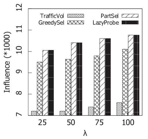
6.3.3. Varying $\lambda$

Figure 11 shows the influence result by varying the threshold $\lambda$ , which determines the influence relationship between billboards and trajectories (in Definition 2.1). We make two observations. (1) With the increase of $\lambda$ , the performance of all algorithms becomes better, because a single billboard can influence more trajectories. (2) PartSel and LazyProbe have the best performance and outperform the GreedySel baseline by at least 8%. This is because the enumerations can easily find influential billboards when the influence overlap becomes larger.

Table 6. Additional test on NYC

	L=100k		L=200k		L=300k
Annealing	6805	0.00%	11777	0.00%	15773	0.00%
TrafficVol	5111	-24.89%	8520	-27.66%	9400	-40.40%
GreedySel	6890	1.25%	12267	5.56%	16108	2.12%
EnumSel	7080	4.04%	13161	11.75%	16570	5.05%
PartSel	7013	3.06%	13215	12.21%	16512	4.69%
LazyProbe	7013	3.06%	13215	12.21%	16512	4.69%

6.3.4. Additional Discussion

We also compared our solution with a meta heuristic algorithm, Simulated Annealing (Annealing), to verify the practical effectiveness. Although Annealing is costly and provides no theoretical bound for our problem, it has been proved to be a very powerful way for most optimization problems and always can find a near optimal solution (Talbi, 2009). Since Annealing is a random search algorithm and its performance is not stable, we run it 50 times for each instance and select the best solution as our baseline. Table 6 reports both the influence value and its relative improvement percentage w.r.t. Annealing for three different choices of budget L. We observe: (1) PartSel and LazyProbe have a very close performance to EnumSel in average. This is because when the overlap between clusters are small, each billboard selected by of PartSel and LazyProbe is less likely to overlap with the billboards in other clusters, and thus the performance of PartSel and LazyProbe would note lose a large accuracy. As discussed later in Section 6.4, EnumSel is very slow to work in practice. (2) PartSel and LazyProbe improve the influence by 6.6% in average as compared to Annealing. (3) TrafficVol which simply uses the traffic volume to select billboards has the worst approximation.

6.4. Efficiency Study

6.4.1. Varying the budget L

Figure 9b and Figure 9d present the efficiency result when budget $L$ varies from 100k to 300k on NYC and LA. As EnumSel is too slow to converge in $10^{4}$ seconds (because the complexity of EnumSel is proportional to $|U|^{5}$ ), we omit it in the figures. We have three main observations. (1) LazyProbe consistently beats PartSel by almost 3 times. (2) The gap between GreedySel and PartSel becomes more significant w.r.t. the increase of L. It is because PartSel has to invoke EnumSel L times for each cluster to construct the local solution for each cluster, so the runtime of PartSel grows quickly with L being increased. (3) TrafficVol is the fastest one with no surprise, because it simply adopts a benefit-based selection.

6.4.2. Varying the trajectory number $\mathcal{T}$

Figure 10b and Figure 10d show the runtime of all algorithms on NYC and LA datasets. We observe that PartSel and LazyProbe scale linearly w.r.t. $\mathcal{T}$ which is consistent with our time complexity analysis; moreover, LazyProbe is around 4 times faster than PartSel.

6.5. Scalability Study

In this experiment we evaluate the scalability of our methods, EnumSel, PartSel and LazyProbe, by varying $|\mathcal{T}|$ (from 400k to 4m) and $|U|$ (from 1k to 10k). Since the effectiveness of GreedySel is not satisfying (as evidenced in our effectiveness study), we do not compare the efficiency of GreedySel. The results are shown in Figure 12a and Figure 12b. We can see that LazyProbe scales very well and outperforms PartSel by 4-6 times. This is because even if the number of billboards is large, LazyProbe does not need to compute all local solutions for each cluster with different budgets, while it still can prune a large number of insignificant computations. Since EnumSel takes more than 10,000 seconds when the billboard number $|U|$ is larger than 2k, its result is omitted in the Figure for readability reason. It also shows that EnumSel has serious issues in efficiency making it impractical in real-world scenarios, while PartSel and LazyProbe scale well and can meet the efficiency requirement.

Summary. (1) Our methods EnumSel, PartSel and LazyProbe achieve much higher influence value than existing techniques (GreedySel, TrafficVol, and Annealing). (2) PartSel and LazyProbe achieve similar influence with EnumSel, but EnumSel is too slow and not acceptable in practice while LazyProbe and PartSel are much faster than EnumSel and can meet the efficiency requirement on large datasets.

6.6. Complementary study

As reported in Section 6, $EnumSel$ could not terminate in a reasonable time for most experiments’ default settings due to its dramatically high computation cost $O(|\mathcal{T}|\cdot{|U|}^{5})$ , we generate a small subset of the NYC dataset to ensure that it can complete in reasonable time, and compare its performance with other approaches proposed in this paper. In particular, we have the default setting of $|U|$ =1000 and $|\mathcal{T}|$ =120k.

Figure 14a and Figure 14c show the effectiveness of all algorithms when varying the budget L and the number of trajectories respectively. From Figure 14a we make two observations: (1) When L is small, the influence of EnumSel is better than that of PartSel and LazyProbe. It is because when only a small number of billboards can be afforded, the enumerations can easily find the optimal set since the possible world of feasible sets is small, whereas PartSel and LazyProbe are mainly obstructed by reduplicating the influence overlaps between clusters. (2) With the growth of $L$ , the advantage of EnumSel gradually drops, while PartSel and LazyProbe achieve better influence; and when the budget reaches 200k, they have almost the same influence as EnumSel. Similar observations are made in Figure 14c.

The efficiency results are presented in Figure 14b and Figure 14d w.r.t. a varying budget and trajectory number. The efficiency of the TrafficVol baseline is not recorded because it is too trivial to get any approximately optimal solution. We find: (1) LazyProbe and PartSel consistently beat EnumSel by almost two and one order of magnitude respectively. (2) EnumSel has the worst performance among all algorithms.

6.6.1. Test on alternative choices of overlap ratio _ij

Here we study how other two alternatives of the overlap ratio described in Section 4.2 affects the effectiveness and efficiency of all algorithms, and the result ( $\theta=0.1$ ) w.r.t. the varying budget is presented in Figure 15.

By comparing Alternative 1 with our choice, we find: (1) from Figure 15a vs. Figure 9a, the GreedySel baseline consistently beats PartSel and LazyProbe under alternative 1, while it is the other way around under our choice. The reason is that this choice only restricts the overlap between clusters rather than billboards. Consequently, some billboards in different cluster should still have a relative high overlap. (2) from Figure 15b vs. Figure 9b, the efficiency of all algorithms are almost the same for both choices.

By comparing Alternative 2 with our choice, we make two observations. (1) From Figure 15c vs. Figure 9a, PartSel and LazyProbe consistently beat GreedySel under both cases. (2) From Figure 15d vs. Figure 9b, the efficiency of all algorithms under our choice is faster than those under alternative 2 by almost one order of magnitude. We interpret the results as, the partition condition of alternative 2 is too strict that $U$ cannot be divided into a set of small yet balanced clusters, thus a larger $|C_{m}|$ is incurred to increase the runtime.

6.6.2. Experiment on an alternative choice of influence probability

Recall Section 2.1 that the influence of a billboard $\mbox{\emph{b}}_{i}$ to a trajectory $t_{j}$ , $\mbox{\emph{pr}}(\mbox{\emph{b}}_{i},t_{j})$ , is defined. Here we conduct more experiments to test the impact of an alternative choice for the influence probability measurement as described in Section 6. The alternative choice is: $\mbox{\emph{pr}}(\mbox{\emph{b}}_{i},t_{j})=\mbox{\emph{b}}_{i}.panelsize/(2*maxPanelSize)$ where $maxPanelSize$ is the size of the largest billboard in $U$ , and we further normalize by 2 to avoid a too large probability, say 1.

The influence result of all algorithms on the NYC dataset is shown in Figure 13. Recall our corresponding experiment of adopting choice 1 in Figure 9a and Figure 10a, we have the same observations: PartSel and LazyProbe outperform all the rest algorithms in influence. To summarize, our solutions are orthogonal to the choice of these metrics.

7. Conclusion

We studied the problem of trajectory-driven influential billboard placement: given a set of billboards $U$ , a database of trajectories $\mathcal{T}$ and a budget L, the goal is to find a set of billboards within L so that the placed ads can influence the largest number of trajectories. We showed that the problem is NP-hard, and first proposed a greedy method with enumeration technique. Then we exploited the locality property of the billboard influence and proposed a partition-based framework PartSel to reduce the computation cost. Furthermore, we proposed a lazy probe method LazyProbe to further prune billboards with low benefit/cost ratio, which significantly reduces the practical cost of PartSel while achieving the same approximation ratio as PartSel. Lastly we conducted experiments on real datasets to verify the efficiency, effectiveness and scalability of our method.

Acknowledgements.

Zhiyong Peng was supported by the Ministry of Science and Technology of China (2016YFB1000700), and National Key Research & Development Program of China (No. 2018YFB1003400). Zhifeng Bao was supported by ARC (DP170102726, DP180102050), NSFC (61728204, 91646204), and was a recipient of Google Faculty Award. Guoliang Li was supported by the 973 Program of China (2015CB358700), NSFC (61632016, 61472198, 61521002, 61661166012) and TAL education.

References

[1] http://oaaa.org/StayConnected/NewsArticles/IndustryRevenue/tabid/322/id/4928.
[2] https://www.statista.com/topics/979/advertising-in-the-us.
[3] http://apps.lamar.com/demographicrates/content/salesdocuments/nationalratecard.xlsx.
[4] http://www.alloutdigital.com/2012/09/what-are-some-advantages-of-digital-billboard- advertising.
[5] http://www.runningboards.com.au/outdoor/relocatable-billboards.
Borgs et al. [2014] C. Borgs, M. Brautbar, J. Chayes, and B. Lucier. Maximizing social influence in nearly optimal time. In SODA, pages 946–957, 2014.
Chen et al. [2015] S. Chen, J. Fan, G. Li, J. Feng, K. Tan, and J. Tang. Online topic-aware influence maximization. PVLDB, 8(6):666–677, 2015. URL http://www.vldb.org/pvldb/vol8/p666-chen.pdf.
Chen et al. [2010] W. Chen, C. Wang, and Y. Wang. Scalable influence maximization for prevalent viral marketing in large-scale social networks. In SIGKDD, pages 1029–1038. ACM, 2010.
Choudhury et al. [2018] F. M. Choudhury, J. S. Culpepper, Z. Bao, and T. Sellis. A general framework to resolve the mismatch problem in XML keyword search. VLDB J., 2018. doi: 10.1007/s00778-018-0504-y.
Feige [1998] U. Feige. A threshold of ln n for approximating set cover. Journal of the ACM (JACM), 45(4):634–652, 1998.
Guo et al. [2017] L. Guo, D. Zhang, G. Cong, W. Wu, and K.-L. Tan. Influence maximization in trajectory databases. IEEE Transactions on Knowledge and Data Engineering, 29(3):627–641, 2017.
Kempe et al. [2003] D. Kempe, J. Kleinberg, and É. Tardos. Maximizing the spread of influence through a social network. In SIGKDD, pages 137–146. ACM, 2003.
Khuller et al. [1999] S. Khuller, A. Moss, and J. S. Naor. The budgeted maximum coverage problem. Information Processing Letters, 70(1):39–45, 1999.
Leskovec et al. [2007] J. Leskovec, A. Krause, C. Guestrin, C. Faloutsos, J. VanBriesen, and N. Glance. Cost-effective outbreak detection in networks. In SIGKDD, pages 420–429. ACM, 2007.
Li et al. [2014] G. Li, S. Chen, J. Feng, K.-l. Tan, and W.-s. Li. Efficient location-aware influence maximization. In SIGMOD, pages 87–98. ACM, 2014.
Li et al. [2015] Y. Li, D. Zhang, and K.-L. Tan. Real-time targeted influence maximization for online advertisements. PVLDB, 8(10):1070–1081, 2015.
Li et al. [2017] Y. Li, J. Fan, D. Zhang, and K.-L. Tan. Discovering your selling points: Personalized social influential tags exploration. In SIGMOD, pages 619–634. ACM, 2017.
Li et al. [2018] Y. Li, J. Fan, Y. Wang, and K.-L. Tan. Influence maximization on social graphs: A survey. IEEE Transactions on Knowledge and Data Engineering, 2018.
Liu et al. [2017] D. Liu, D. Weng, Y. Li, J. Bao, Y. Zheng, H. Qu, and Y. Wu. Smartadp: Visual analytics of large-scale taxi trajectories for selecting billboard locations. IEEE Transactions on Visualization and Computer Graphics, 23(1):1–10, 2017.
Liu et al. [2013] Y. Liu, R. C.-W. Wong, K. Wang, Z. Li, C. Chen, and Z. Chen. A new approach for maximizing bichromatic reverse nearest neighbor search. Knowledge and Information Systems, 36(1):23–58, Jul 2013.
Murtagh [1983] F. Murtagh. A survey of recent advances in hierarchical clustering algorithms. The Computer Journal, 26(4):354–359, 1983.
Talbi [2009] E.-G. Talbi. Metaheuristics: from design to implementation, volume 74. John Wiley & Sons, 2009.
Tang et al. [2014] Y. Tang, X. Xiao, and Y. Shi. Influence maximization: Near-optimal time complexity meets practical efficiency. In SIGMOD, pages 75–86. ACM, 2014.
Wagner and Wagner [1993] D. Wagner and F. Wagner. Between Min Cut and Graph Bisection, pages 744–750. Springer, Berlin, Heidelberg, 1993.
Wang et al. [2017] S. Wang, Z. Bao, J. S. Culpepper, T. Sellis, M. Sanderson, and X. Qin. Answering top-k exemplar trajectory queries. In ICDE, pages 597–608. IEEE, 2017.
Wang et al. [2018a] S. Wang, Z. Bao, J. S. Culpepper, T. Sellis, and G. Cong. Reverse k nearest neighbor search over trajectories. IEEE Trans. Knowl. Data Eng., 30(4):757–771, 2018a.
Wang et al. [2018b] S. Wang, Z. Bao, J. S. Culpepper, Z. Xie, Q. Liu, and X. Qin. Torch: A search engine for trajectory data. In SIGIR. ACM, 2018b.
Wong et al. [2009] R. C.-W. Wong, M. T. Özsu, P. S. Yu, A. W.-C. Fu, and L. Liu. Efficient method for maximizing bichromatic reverse nearest neighbor. PVLDB, 2(1):1126–1137, 2009.
Zhou et al. [2011] Z. Zhou, W. Wu, X. Li, M. L. Lee, and W. Hsu. Maxfirst for maxbrknn. In ICDE, pages 828–839. IEEE, 2011.

Trajectory-driven Influential Billboard Placement

Abstract.

Keywords:

1. Introduction

2. Preliminary

2.1. Problem Formulation

Definition 2.1.

Example 2.1.

Definition 2.2.

Theorem 2.1.

Proof.

2.2. Related work

3. Our Framework

3.1. Baselines

3.1.1. A Basic Greedy Method

Theorem 3.1.

Proof.

3.1.2. Enumeration Greedy Algorithm

Example 3.2.

3.2. A Partition-based Framework

Example 3.3.

4. Partition based Method

4.1. Partition based Selection Method

Definition 4.1.

Example 4.1.

4.2. θ\theta-partition

Definition 4.2.

Definition 4.3.

Lemma 4.1.

Proof.

Theorem 4.2.

Proof.

4.3. Finding a θ\theta-partition

5. Lazy Probe

5.1. The Lazy Probe Algorithm

Example 5.1.

5.2. Theoretical Analysis

Theorem 5.1.

Proof.

Lemma 5.2.

Lemma 5.3.

Proof.

Lemma 5.4.

Proof.

6. Experiments

6.1. Experimental Setup

6.2. Experiments

6.2.1. Choice of θ\theta-partition

6.3. Effectiveness Study

6.3.1. Varying the budget L

6.3.2. Varying the trajectory number |𝒯||\mathcal{T}|

6.3.3. Varying λ\lambda

6.3.4. Additional Discussion

6.4. Efficiency Study

6.4.1. Varying the budget L

6.4.2. Varying the trajectory number 𝒯\mathcal{T}

6.5. Scalability Study

6.6. Complementary study

6.6.1. Test on alternative choices of overlap ratio ij

6.6.2. Experiment on an alternative choice of influence probability

7. Conclusion

Acknowledgements.

References

4.2. $\theta$ -partition

4.3. Finding a $\theta$ -partition

6.2.1. Choice of $\theta$ -partition

6.3.2. Varying the trajectory number $|\mathcal{T}|$

6.3.3. Varying $\lambda$

6.4.2. Varying the trajectory number $\mathcal{T}$

6.6.1. Test on alternative choices of overlap ratio _ij