C-P-T anomaly matching in bosonic quantum field theory and spin chains
Abstract
We consider the nonlinear sigma model with the -term and its linear counterpart in 1+1D. The model has discrete time-reflection and space-reflection symmetries at any , and enjoys the periodicity in . At it also has a charge-conjugation -symmetry. Gauging the discrete space-time reflection symmetries is interpreted as putting the theory on the nonorientable manifold, after which the periodicity of and the symmetry at are lost. We interpret this observation as a mixed ’t Hooft anomaly among charge-conjugation , parity , and time-reversal symmetries when . Anomaly matching implies that in this case the ground state cannot be trivially gapped, as long as , and are all good symmetries of the theory. We make several consistency checks with various semi-classical regimes, and with the exactly solvable XYZ model. We interpret this anomaly as an anomaly of the corresponding spin-half chains with translational symmetry, parity and time reversal (but not involving the -spin symmetry), requiring that the ground state is never trivially gapped, even if spin symmetry is explicitly and completely broken. We also consider generalizations to models and show that the -- anomaly exists for even .
I Introduction
Spin chains are often effectively described by nonlinear or linear sigma models in 1+1D. In particular, Haldane showed [1, 2] that a quantum Heisenberg anti-ferromagnet in the limit of a large spin , reduces to the nonlinear sigma model in 1+1D with the target space (the Bloch sphere). This model is referred to, conventionally, as the nonlinear sigma model. Importantly Haldane showed that a natural topological -term given by arises from the microscopic model, and argued that the integer and half-integer spin fall separately into two universality classes since the partition function of the model is invariant under the shifts of by . Indeed the spin-1/2 Heisenberg antiferromagnet is exactly solvable by the Bethe ansatz, and is gapless, while the AKLT model [3] as well as numerous simulations of the nonlinear sigma model show a gapped spectrum, often referred to as the Haldane gap.
The different behavior of the two regimes can be traced back to the Lieb-Schultz-Mattis (LSM) theorem [4, 5, 6], which states that in the half-integer spin case, spin chains either have to be gapless or break translational symmetry [7]. No similar statement exists for integer spin systems. The underlying reason of the LSM theorem is that the spin symmetry acts projectively on the half-integer spins.
It has recently come to light that the LSM theorem manifests itself as ’t Hooft anomaly in the effective theory (see e.g. Refs. [8, 9, 10] which touch upon this connection). The ’t Hooft anomaly can be summarized as an inability to gauge a particular symmetry group without introducing non-local terms in the action. Unlike quantum anomalies, ’t Hooft anomalies do not invalidate the global symmetry, but instead give powerful constraints on the IR physics. The ’t Hooft anomaly matching condition was originally proposed for continuous chiral symmetry of gauge theories with massless fermions [11, 12, 13], where it was used to predict that chiral symmetry must be broken or the system must be in the conformal phase.
How ’t Hooft anomalies constrain the infrared physics can be intuitively explained as follows (We review the anomaly matching more precisely in the Appendix A). For the sake of simplicity we will assume the theory possesses a symmetry group . Gauging a symmetry group amounts to chopping up the space-time manifold into separate pieces, and stitching them back together up to a symmetry transformation in . This procedure can also be thought of as endowing a system with twisted boundary conditions in the group in various directions. If, in the presence of such twist, no local formulation of the theory is invariant under the group, then it must be that the boundary twists in the group have excited a state in the group . This can only happen if the ground state is nontrivial. In this case, we say that there exists a mixed ’t Hooft anomaly between the global symmetry group and .
In order to gauge symmetries with ’t Hooft anomalies, nonlocal terms in the action are needed by definition. A typical way to achieve this is by extending the system into an auxiliary “bulk” direction which is in the symmetry-protected topological (SPT) phase. The anomaly inflow [14] from the bulk SPT phase shows that the ’t Hooft anomaly is renormalization-group invariant. The consequence of this anomaly matching condition is that the vacuum cannot be trivially gapped, and must either have a long-range order (i.e. spontaneous symmetry breaking), long-range entanglement (i.e. topological order) or infinite correlation length (i.e. gapless excitations) [15, 16, 17, 18, 19]. We emphasize that the auxiliary SPT bulk phase is not necessary to realize “the boundary” system, and is a priori a mathematical tool. Nevertheless a bulk may exist, and systems which are ’t Hooft anomalous may be realized as a boundary of some SPT bulk state.
In previous studies [20, 21, 22], it was shown that the sigma model at has an ’t Hooft anomaly involving two-form gauge field between symmetries and charge conjugation . For , it is the nonlinear sigma model and reproduces the Haldane conjecture for half-integer spins, so this ’t Hooft anomaly matching corresponds to the conventional LSM theorem requiring the spin- (or rather it’s subgroup) and lattice translational symmetries. Similar ’t Hooft anomalies involving discrete symmetries have also been of recent interest in various gauge theories [20, 23, 24, 25, 26, 27, 28, 29].
In this paper, we show that a certain class 1+1D systems with a topological term have another kind of ’t Hooft anomaly which does not require the spin symmetry to be preserved at all. More concretely, we show that the nonlinear sigma model at has a mixed ’t Hooft anomaly for the time-reversal , spatial reflection , and charge conjugation symmetries. We call this ’t Hooft anomaly as a -- anomaly. Ref. [9] also discussed11 1 We thank Z. Komargodski for pointing out this reference to us, which motivated our current work. anomalies which do not involve the spin symmetry. However these are claimed to be IR emergent anomalies, involving spatial translations only. In contrast the anomaly we discuss here are fundamental anomalies of the underlying system, of the LSM-type, and they involve time-reversal and parity as well as spatial translations. The implication therefore is that the -- anomaly is a different kind of LSM theorem for spin chains which preserve parity, time reversal, and lattice translational symmetries [30, 31], but not necessarily the spin symmetry.
To show its existence, we put the theory on the non-orientable manifold , along with certain boundary conditions on the fields, which amounts to gauging the and symmetry (see also [32, 33, 34, 35, 36, 37, 38, 39] for related works). We find that the topological charge of the sigma model becomes quantized to half integers on , and the charge conjugation symmetry at is explicitly broken. Furthermore we show that there is no local counterterm to eliminate this breaking. In addition we generalize the -- anomaly to the case of model when is even.
We check that the constraint by the anomaly matching is consistent with the known results about our model and what is known about the corresponding spin systems, such as the XXZ and the XYZ model which are exactly solvable. We also discuss consistency of the anomaly with the semi-classical regimes. This will be helpful for clear understanding of how the anomaly matching is realized in this system. Finally we briefly discuss the ’t Hooft anomaly of the underlying lattice system.
The paper is organized as follows: In Sec. II, we explain the nonlinear sigma model and its discrete symmetries , , . In Sec. III, we compute the ’t Hooft anomaly for , , and symmetries, and discuss semi-classical limits of the system. In Sec. IV, we discuss the generalization of the -- anomaly for the model for even . In Sec. V we discuss the anomaly in the underlying lattice system. We give conclusions in Sec. VI. In Appendix A, we give a brief review on anomaly matching.
II nonlinear sigma model
We will consider the (i.e. target space) nonlinear sigma model in two-dimension with a term. The Lagrangian is
| (1) |
where is the unit vector, . The second term () is the topological theta term of the action, where on a closed orientable manifold. As a consequence, the partition function is periodic with respect to .
We will first focus on model (1). However it is worth noting that everything we say will hold also for
| (2) |
where is a scalar doublet, is the gauge-covariant derivative, is the field strength, is a gauge invariant potential of obeying the relevant symmetries. The two models are equivalent if we set and the term is dropped.
The system (1) has a time-reversal22 2 How time-reversal – an anti-unitary symmetry – acts in the Euclidean path integral is slightly subtle and is addressed in the appendix C. The result is simple enough, as it amounts to the reversal in time in the Euclidean Lagrangian (without complex conjugation), without affecting the limits of the time integration. and parity (or equivalently – reflection) symmetry
| (3a) | |||
| (3b) | |||
at any . Notice that we use the asterisk on . This is because this transformation has two interpretations: either as a symmetry of the field theory or a bond-centered parity symmetry of the underlying spin-chain.
Let us explain this a bit more. The above theory is believed to be an effective theory of an anti-ferromagnetic spin-chain. The chain has a translational symmetry which is a symmetry of the Hamiltonian. The continuum limit then requires that spin at site is related to the Néel vector at the same site by , i.e. the Néel vector is staggered by a different sign on the two sublattices. The translation symmetry by a single lattice unit therefore changes the sign of the Néel vector. So in the field theory description (1), this translational symmetry ( ) is mapped to the charge conjugation symmetry
| (4) |
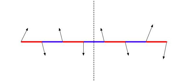
and it is only a symmetry of (1) when . Hence the arbitrary corresponds to the absence of the translational symmetry. Microscopically the lack of translational symmetry is sketched in Fig. 1, where red and blue bonds denote different anti-ferromagnetic interactions. Notice that the parity around the midpoint of any link is a good symmetry. This parity acts by interchanging the two sub-lattices, which has the effect of changing the Néel order parameter . So the operator is a link-centered parity of the underlying microscopic theory33 3 The situation is reminiscent to identifying a field-theory symmetry with the microscopic -symmetry as in Ref. [40]..
On the other hand could also correspond to the vertex centered reflection followed by a translation symmetry as well. Since the translation symmetry is mapped to the -symmetry in field theory we would call the combination of the two the symmetry.
In fact the model (1) is equivalent to the model, where instead of fields we write the action in terms of the — a complex doublet, and — the auxiliary gauge field. It can be checked (see below) that the symmetry acts on the theory as the symmetry, where is charge conjugation. Indeed, the sigma model (1) has the invariance: We have , by Lorentz invariance, and in (3) is the partner of the time-reversal symmetry .
III Gauging and symmetries
We will now show that at there exists a mixed ’t Hooft anomaly between and symmetry. To see this, let us first place the system on a -torus, so that the coordinate and . The fields obey boundary conditions
| (5) |
The path integral over all the possible configurations with this boundary condition gives the ordinary partition function of the system.
Now we wish to gauge the and symmetries (3) in order to detect the ’t Hooft anomaly involving them. To that end, we put the theory on a non-orientable manifold by imposing the boundary conditions
| (6a) | ||||
| (6b) | ||||
We interpret these boundary conditions as putting the background gauge fields for the symmetries (3) along the two cycles of the torus44 4 The twist in the in the temporal direction can be interpreted as an insertion of a parity symmetry operator into the thermal partition function. This can be interpreted as the presence of a nontrivial parity gauge field in the temporal direction. Similarly spatial gauge fields were constructed in Ref. [41], to generalize the notion of gauge fields in the spatial directions. We apply the same logic to the time-reversal symmetry, and implement time reversal at some point along the spatial circle. However we here emphasize that since the time-reversal symmetry is an antiunitary symmetry, we do not know whether a Hilbert space interpretation of twists exists, i.e. whether it makes sense to gauge the -symmetry with a temporal gauge field. Part of the problem is that there is a difficulty of defining the -operator insertion into the partition function, because trace of the antilinear operator is not invariant under the basis change. This is why we circumvent this problem by applying the gauge field of the symmetry along the spatial direction.. Quick thought reveals that the boundary conditions render the manifold topologically equivalent to a disc with any two opposing points on its boundary identified. This manifold is a projective plane and is non-orientible.
III.1 Topological charge on
We wish to show that with these boundary conditions (6) the quantization of topological charge is in half-integer units. Namely the topological charge is . In fact we can see this already by considering to be topologically a disk, with opposing points on the boundary of the disc identified up to a transformation . An example of such a configuration is given by , where we parametrize the disk by the stereographic projection for and (see Fig. 2). The topological charge is
| (7) | |||||
This configuration indeed has a half-integer winding number. This configuration is sketched in Fig. 2, and it obviously covers only the half of the target space .

Let us now prove that all configurations have a half-integral winding number. To do this it is useful to use the parametrization, i.e. to define
| (8) |
where with the constraint . Here, is the Pauli matrix, . This parametrization has a gauge symmetry . Then it can be shown that
| (9) |
where we defined
| (10) |
This is a gauge field.
Note that in this parametrization, the transformation corresponds to , where ∗ denotes complex conjugation. Therefore we have that and transform as
| (11) | ||||
| (12) |
while
| (13) | ||||
| (14) | ||||
| (15) | ||||
| (16) |
The transformation is the usual transformation of the gauge fields under time-reversal55 5 An easy way to see this is that the coupling of the gauge field to the conserved current must be invariant under the transformation. Now under the -transformation the charge density is invariant , however the spatial current flips sign under .. On the other hand the transformation is not what we usually call parity transformations. Instead in this context it is identified with (see discussion below (3)).
Once we have established the transformations, we can shift our attention entirely to the gauged linear sigma model, of the type (2), and everything we say below is equally applicable to this case.
The boundary conditions (6) turn into
| (17a) | ||||
| (17b) | ||||
and
| (18a) | ||||
| (18b) | ||||
| (18c) | ||||
| (18d) | ||||
By plugging into the first equation of (17), and into the second equation, we get
Complex conjugating the second equation, and plugging into the first, we get
| (19) |
hence we conclude that
| (20) |
Similarly, by putting in the first, and in the second equation of (17) we get
| (21) |
The result is summarized in Fig. 3.
Now we are ready to evaluate the -term on the manifold which arose from gauging the and symmetries. For this purpose we will consider to be a filled rectangle depicted in Fig. 3, where horizontal axis represents space and vertical axis represents Euclidean time. The upper and lower edges of the rectangle are identified modulo the transformation which reverses space, while the left and right edges are identified modulo -transformation which reverses time, which is indicated by the arrows of the respective edges. We write
| (22) |
where the integral on the right is along the boundary of our open rectangle . Now we obtain that
| (23) | |||||
where we identified the appropriate and relations on the upper/lower and left/right edges of Fig. 3 respectively. This shows that all the configurations with boundary conditions (6) have a half integral winding number.
III.2 Non-periodicity in and the mixed ’t Hooft anomaly between and
As we already discussed the model (1) has and symmetries for any value of . We have showed above how we can put background gauge fields for the and symmetry. However the model also has another symmetry when , i.e. the charge conjugation . When , the -symmetry is a symmetry because the winding number is quantized in integer units. Similarly the partition function is a periodic function of because of this quantization.
However as we already saw when we gauge the and symmetries, the quantization of topological charge is in half-integer units, and the periodicity of the partition function with respect to is ruined. For this has a consequence that the symmetry is not a symmetry in the presence of the and gauge fields. Equation (23) shows that the partition function on the non-orientable manifold , , is changed under as
| (24) |
with , and the symmetry is broken while it is a good symmetry on any orientable manifolds.
We interpret this as the mixed ’t Hooft anomaly between , , and at . For that purpose, we must check that the anomaly (24) is not fake, i.e. it cannot be canceled by the local counterterm to the action. To show it, we have to look at all the possible D local actions as we shall do below.
In fact, the possible local counterterm is characterized by the topological action depending on the gauge fields for , , and it is given by
| (25) |
Here, is the real-vector bundle on whose section defines the real-vector field , and is the first Stiefel-Whitney class, which is the obstruction of orientation.
Let us explain the notation a bit. We can consider to be the gauge field for the and symmetry. So if the integral of over some 1-cycle is nontrivial, it means that a transformation reversing the orientation of space-time and flipping is applied as one traverses the cycle. Further, notice that what we have shown in the previous section is that
| (26) |
The right hand side is trivial on an orientable manifold, as it should be.
The second Stiefel-Whitney class is also a candidate for the counterterm. On -dimensional manifolds, however, there is a relation due to vanishing of the second Wu class, and thus this topological action (25) is the unique possible counterterm (see, e.g., Appendix of Ref. [42]). Here, is the cup product. The above integral does not vanish on the non-orientable manifold, while it always vanishes on orientable manifolds modulo . The charge conjugation does not change the counterterm at all, and thus it cannot eliminate the anomaly (24).
Finally notice that if we continuously deform a theory by changing its term by , we generate a counterterm . If the theory is defined on a manifold with boundaries, the partition function is supplemented with a factor , which requires that the boundaries are carrying Kramers’ doublets [42].
We therefore have an ’t Hooft anomaly between , and symmetries at . The anomaly matching claims that the system must either
- •
break , , or symmetry spontaneously66 6 If we assume the theory to be relativistic, and if we assume that the ground state does not break Lorentz symmetry spontanously, we must have that if is broken, then must also be broken.,
- •
have massless excitations (conformal behavior), or
- •
have long-range entanglement (topological order).
For 1D spin chains, it is shown that the topological order does not appear [30]. Therefore, we can conclude that the system is conformal or breaks one of the discrete symmetries if the field theory appears as a low-energy description of the spin model. When the field theory does not have the UV Hamiltonian of the 1D spin systems, however, this additional constraint does not apply. In fact we will show that a topological phase can arise as a limit, in section Sec. III.3. This scenario is quite esoteric however, and arises only if the charge-2 Higgs field has a runaway potential. Since we are unaware of of a scenario which would contain a charge-2 condensing Higgs field77 7 It may be possible to obtain such exotic phases by realizing 1D systems as domain walls of higher dimensional systems, as in Refs. [43, 22] (see also Ref. [44]), let alone one with a runaway potential, we will exclude this possibility from our considerations.
We can make a stronger conclusion by taking into account the spin rotation symmetry . In Refs. [21, 22], it is shown that there is a mixed ’t Hooft anomaly between and , which derives the conventional LSM theorem. Therefore, we must match both the - and -- anomalies for the sigma model at . This means that, for instance, the spontaneous time-reversal breaking is not enough to match the anomaly, because it matches the -- anomaly but does not match the - anomaly. By taking into account the Coleman-Mermin-Wagner theorem [45, 46], the symmetry cannot be broken spontaneously in two-dimension, and the anomaly is matched by
- •
spontaneous breaking of , or
- •
conformal behavior
It is also interesting to consider the situation where symmetry is broken down to some discrete subgroup explicitly by additional interactions, and let us assume that there is the mixed anomaly between and as a remnant of the - anomaly. The - anomaly and the -- anomalies are matched by
- •
spontaneous breaking of ,
- •
spontaneous breaking of , and of or , or
- •
conformal behavior
III.3 Consistency checks of the anomaly
III.3.1 Consistency with the XYZ model
We will now comment on the XYZ model which is exactly solvable, and see how its phases match the anomaly. This will provide more insight about anomaly matching for strongly-coupled cases. The Hamiltonian is given by
| (27) |
with the periodic boundary condition, , and this system is exactly solvable by the Bethe ansatz (see, e.g., Refs. [47, 48]). This Hamiltonian still have a discrete subgroup88 8 is the Klein four group and is generated by rotations of around any two axis. of symmetry, so it is not completely generic. The model also possess, in addition to the spin symmetry, the translational symmetry which is mapped to in the field theory language, the time-reversal symmetry and the bond-centered parity . Further in addition to the CPT mixed ’t Hooft anomaly anomaly, it also possesses the mixed anomaly between99 9 See [10] and the Appendix B. and .
Still, it is insightful to compare our anomaly with its ground-state structures. When , this is called the XXZ model. It preserves and its ground-state properties are parametrized with as follows: For , the ground state is doubly degenerate, which is the ferromagnetic phase1010 10 Those ground states are given by and . [48]. The anomaly is matched by spontaneous breaking. It also breaks the down to , and the spontaneous breaking of and is required to match both - anomaly and -- anomaly1111 11 Note that the effective theory of the ferromagnets is not described by the relativistic theory in the IR (see e.g. [49]) because of the spin Berry phases. Hence breaking without breaking is allowed.. For , the ground state is nearly degenerate at finite , and the difference between them vanishes as in the thermodynamic limit [48]. This is the antiferromagnetic phase1212 12 In the antiferromagnetic Ising limit, , those two states are given by for even , which breaks the translational symmetry spontaneously (and symmetry) in the thermodynamic limit. Therefore, the anomaly is matched by and breaking. When , we have gapless excitations [48], called spinon, spin-wave and bound-state excitations, and they match the anomaly. For the most general XYZ model, it is sufficient to consider the case since it is known that the spectrum of the XYZ Hamiltonian is invariant under the flip of two ’s. This system is gapped, but we can construct the nearly degenerate state, whose energy difference from the ground-state energy rapidly decreases in the thermodynamics limit [48]. Therefore, the anomaly is matched by the spontaneous symmetry breaking. Depending on the parameters and (all which are different), the system either is in a ferromagnetic or anti-ferromagnetic phase. The earlier phase breaks the -symmetry as well as and the latter breaks and translational symmetry.
III.3.2 Consistency with semi-classics
Let us now explore some semi-classical limits. It is believed that the model (1) at is described by the Wess-Zumino-Witten conformal theory. This is consistent with the previously found ’t Hooft anomaly in the sigma model between and symmetries [21, 22].
As we have seen, however, that ’t Hooft anomaly exists even if the global symmetry is reduced down to its improper part, as long as parity and time-reversal are good symmetries of the theory. We will now explore deformations which will keep the -- anomaly intact, and demonstrate several regimes how the anomaly manifests itself. Thus, we focus on an (Euclidean) action
| (28) |
where – a complex SU(2) doublet, is the gauge field strength of the dynamical gauge field , and is the covariant derivative. is a gauge invariant potential for the -scalars, which also preserves the -symmetry defined as
| (29) |
For simplicity of notations to construct such , let us define the gauge-singlet fields
| (30) |
and are related by , but we do not require that is unity. The transformation changes the sign of all the components of , while does not change under . Hence, to preserve the C-symmetry, we must have that the potential is an arbitrary function of and of the product for any , i.e.
| (31) |
Such a potential in generic case completely destroys the symmetry. Yet, our consideration guarantees that the ground state cannot be trivially gapped.
Classically speaking, if the potential is minimized at any nonzero value of it must break the -symmetry, and have at least two classically degenerate vacua. On the other hand, if a potential minimizes at we must have . Then, semi-classically speaking, we can integrate out the massive -fields, and obtain an effective pure-gauge theory (quantum Maxwell theory) at . This theory again breaks -symmetry at , as is well known.
In the end let us consider another, purely quantum, scenario. Let us add a scalar with charge under the gauge group, i.e. a field which has a kinetic term given
| (32) |
Now if we wish to have the same -- anomaly, we must first check if the global symmetries are the same. To that end, consider a gauge-invariant operator
| (33) |
Under the charge conjugation, is mapped to , and . Now let us apply the -transformation twice, then the above gauge-invariant operators are transformed as
| (34) |
The symmetry is no longer a symmetry, but a symmetry if is an odd integer. Since we wish to consider possible deformations of the original model, without changing the global symmetries, we choose to be even.
Now the global symmetry group is unchanged, and the -- anomaly is present, so that we cannot have a trivially gapped state. Let us now take the mass-squared of the charge- scalar to be large and negative, so that it condenses and Higgses the gauge field. In other words we can write , where we can ignore the fluctuation of and set it to be constant and large. Then the kinetic term gives
| (35) |
Minimization of this term forces the gauge field to be a gauge field:
| (36) |
However, the theory can have gauge-vortices for which winds by as the nexus of the vortex is traversed, and the above condition (36) is satisfied only outside the vortex cores. The vortex therefore must have a fractional flux, because for the single-vortex
| (37) |
Because the vortices carry fractional flux, they can only occur in bunches of to satisfy the correct boundary condition for the thermal partition function. Furthermore, they will each couple to the -angle as . If we naively sum over all such vortices by the dilute-instanton gas approximation (, i.e., ignoring their exponentially small interaction), we get that the energy density is given by
| (38) |
Here, is the action of the fractional vortex. The above expression is not periodic with respect to . This is because we have not taken into account the fact that only bunches of vortices can contribute to the partition function. To achieve that, we must impose the constraint that by introducing the Kronecker’s delta, which it can be written as the Fourier series
| (39) |
Notice that the above integer combines with the -angle, and amounts to replacing . Notice that the -symmetry is now a symmetry at only if we take . As a result, we obtain that the ground-state energy is
| (40) |
At the vacua and are degenerate. Since they are also related by the symmetry, we conclude that the system breaks -symmetry.
Let us now take the limit of . In this case -symmetry is restored since the fugacity of the fractional vortex vanishes, and we have an apparent contradiction with the anomaly. However notice that the quanta are completely noninteracting now, and therefore become fractionalized excitations, so that there is still a long-range topological order. In other words, the constraint (36) holds true everywhere on the spacetime in this limit, and thus the low-energy field theory is described a nontrivial topological field theory, called BF theory.
However, as we commented before, it is doubtful that such an instability is of physical relevance. In order to be relevant, one would have to obtain a form of a runaway potential for the Higgs field. We only mention such a phase as a curiosity.
IV Generalization of -- anomaly to model for even .
In order to construct the appropriate -symmetry, we want to define
| (41) |
where is an matrix. If we apply the above transformation twice we get
| (42) |
In order for the -symmetry to be a symmetry we must require that – an element of the center. If this is the case with the nontrivial center, , then the -symmetry will act projectively and we may have an ’t Hooft anomaly.
The condition translates to
| (43) |
Since , this is equivalent to
| (44) |
by taking the transpose of the both sides. In order for both to be true we must have that .
For odd we have that the only element of the center with such a property is a trivial element . So we conclude that there is no corresponding -symmetry in the case for which there is a -- anomaly if is odd.
For -even we have that the element is always in the center, hence it is possible to satisfy this condition. In fact the condition amounts to finding an anti-symmetric element. Indeed if we pick
| (45) |
it is clear that this condition is satisfied. We can then follow the same steps as in Sec. III.1 and show that there exists a -- anomaly.
V Comment on the microscopic spin chains
In this paper we do not dwell on the microscopic theories. However we would like to take a moment to comment on the appearance of the anomaly in the underlying lattice system. If we take the lattice to consist of spin-half particles on sites, then each site has a double-degeneracy (Kramers’ degeneracy) as long as time-reversal is a good symmetry (denoted by blue dots in Fig. 4). Now we note that such a system can be though of as SPT phases (red lines) protected by time reversal symmetry, which end on the blue dots. Such an SPT phase in 1+1D was discussed in [18], and its action must include the term on the over every other link of the chain1313 13 We have a path-integral picture of the chain in mind. In other words, the 1D chain is supplemented with the time direction. The integral between the link and is then interpreted as the integral over all time, and bounded by the spatial positions of and vertex.. We now observe that translation symmetry (which maps to the -symmetry in the continuum) generates exactly the change in the action
| (46) |
which is precisely the same as (25) discussed as in the context of the continuum. We therefore conclude that the system has the microscopic system with the same type of anomaly as its effective theory, as expected.
We have already discussed how the consistency of the XYZ model with the anomaly. However in this case the symmetry is not fully broken, but is reduced to the , which is still ’t Hooft anomalous with translation symmetry. To truly test the predictions of the -- anomaly, we would like to break the symmetry completely. We suggest the spin chain with the Hamiltonian
| (47) |
where , which we call the skewed-XYZ model1414 14 Notice that both first and second term leave invariant a ’t Hooft anomalous , and only the combination of the two break the symmetry completely.. It becomes the XYZ model when , but it completely breaks in generic cases.
VI Conclusion
We have discussed here the appearance of the mixed ’t Hooft anomaly between charge conjugation , parity , and time-reversal symmetries for the two-dimensional nonlinear sigma model at , as well as a general Abelian-Higgs model with two scalar fields. Since it does not involve the symmetry, the anomaly matching constraint for this system exists even if we introduce terms to break the symmetry completely, so long as , , and are good symmetries of the perturbation. As a consequence of anomaly matching, the system cannot have the trivial gapped phase, and thus it must break , , or spontaneously, have massless excitations, or have nontrivial topological order.
The -- anomaly discussed here should be viewed as the generalization of the LSM theorem to spin-systems without the global spin symmetry. This -- anomaly is the field-theoretic description of the LSM theorem involving and the lattice symmetries, discussed in Ref. [30, 31].
An interesting future perspective would be to explore such anomalies in higher dimensional spin-half systems. In fact a hint that such an anomaly indeed exists is contained in the observation that a rectangular spin-1/2 system can be viewed as a series of spin-1/2 chains, each of which can only be realized as a boundary state of an SPT phase protected by the “” symmetries discussed here. Therefore such a D system can be viewed a staggering of the 1+1D trivial and non-trivial SPT phases living between the chains. Such a setup breaks the translation symmetry shifting the stack of spin-1/2 chains, and implies that there should be an anomaly involving spatial reflections, translations and time reversal in systems as well. If this is the case, then a similar argument can be made for D spin systems on a cuboid lattice. We leave this interesting problem for the future.
Another interesting extension of this work is to include the fermionic degrees of freedom, in particular extending the model to a supersymmetric one. The supersymmetric nonlinear sigma model has a classical chiral symmetry reduced to by instanton effects, and is believed to be spontaneously broken. Should gauging space-time symmetries (which should be possible unless discrete space-time symmetries are themselves ’t Hooft anomalous) lead to fractional quantization of topological charge, the chiral symmetry would be eliminated completely, implying a mixed ’t Hooft anomaly between discrete space-time symmetries and discrete the chiral symmetry.
Acknowledgements.
We thank Gerald Dunne and Zohar Komargdoski for their useful comments on the initial draft of the paper. We also benefited greatly from the discussions with Costas Bachas, Gerald Dunne, Zohar Komargdoski, Anders W. Sandvik, and Mithat Ünsal. We also appreciate Ken Shiozaki and Yohei Fuji drawing our attention to Refs. [30, 31]. The authors would also like to thank the hospitality at the KITP institute and the organizers of the “Resurgent Asymptotics in Physics and Mathematics” workshop where a part of this was done. The work at KITP is supported by National Science Foundation under Grant No. NSF PHY-1125915. The work of Y. T. is supported by RIKEN Special Postdoctoral Researchers Program.Appendix A ’t Hooft anomaly matching
In this appendix, we give a brief review on the anomaly matching condition.
Let us consider quantum field theory on -dimensional spacetime (i.e. with space dimension) with a global symmetry . We introduce the background -gauge field to the system, and denote the partition function as , then the ’t Hooft anomaly is defined as the gauge non-invariance on the phase of the partition function:
| (48) |
Here, is the gauge parameter, is the gauge variation of by , and is the -dimensional local functional of and .
The working assumption, which can be checked in each concrete example, is that the ’t Hooft anomaly can be canceled by anomaly inflow from the -dimensional SPT phase protected by the symmetry . Such SPT phase is characterized by -dimensional action of the topological -gauge theory , and the assumption claims that
| (49) |
when the SPT phase has the -dimensional boundary. As a result, the combined system,
| (50) |
becomes -gauge invariant. The SPT action cannot be influenced by the RG flow at the boundary, as it is a gapped phase and contains no propagating degrees of freedom. In other words, whatever the low-energy effective theory of is, it must cancel the gauge non-invariance of coming out of the boundary, so the low-energy effective theory should have the same ’t Hooft anomaly of the original theory. This is the ’t Hooft anomaly matching condition.
By taking the ultimately low-energy limit, we can claim that the anomaly should be matched by massless excitations or the degeneracy of the ground states since we can integrate out the massive excitations. The vacuum degeneracy may be created by the spontaneous symmetry breaking of a global symmetry group or the topological order. So a ’t Hooft anomaly matching requires
- •
spontaneous symmetry breaking of some part of ,
- •
conformal behavior, or
- •
topological order.
The ’t Hooft anomaly provides a nontrivial consequence on the nonperturbative dynamics of interacting quantum field theories.
Appendix B mixed anomaly
We here briefly discuss the mixed anomaly between and the symmetry of the effective field theories of spin chains given by (2). The group is the subgroup of the spin which is generated by rotations around the and axis of the spin. The consequences of this anomaly appeared in [10]. We here want to put the observations in the context of the ’t Hooft anomaly matching.
The group has four elements, which are the unit element along with rotations around the three axes Néel vector axes , which we label as . The group elements act projectively on the -field as elements .
Now let us think about adding the gauge field for the two -s of the . The associated gauge fields we take to be and . Notice that under the -symmetry changes sign, while is invariant.
Let us now think of adding the gauge field along the -direction1515 15 We reserve the numbers for space-time indices, and for Néel vector andA^y2e^i∫_γ_1 A^x=e^i∫_γ_2A^y=-1γ_1,22uU(1)C, ~ C U(1)2π2π2πiA^x,y→A^x,y+dφ^x,yp∈Ze^2i∫_γA^x,y=1γA^x,yZ_2A^x_1A^y_2ipπpp=1pp=0CCCCCA_CZ_2CΣ∂Σ=T^2K_4-C
Appendix C Symmetries: from Hilbert space to path-integrals
C.1 Unitary symmetries
To start we first define a Euclidean time matrix element
| (55) |
To represent the matrix element as the path integral, we typically choose a particular complete basis of states, typically coordinate eigenstates, which we will denote as . Note that the state itself may depend on space — i.e. an index labeling coordinates – but since we are working in the Heisenberg picture (in Euclidean time) the state has no time dependence. We also have the completeness relation
| (56) |
where is the appropriate measure on the coordinate space. The matrix element (55) can then be written as
| (57) |
where and where1616 16 The “link action” strictly depends also on . However in the limit , the dependence on dependence will be irrelevant, so we omit it for simplicity.
| (58) |
Now let us do a symmetry transformation , where is a unitary operator. The matrix element (55) is invariant, because commutes with the Hamiltonian. How is this invariance manifested in the path-integral.
Let
| (59) |
Then we have
| (60) |
Further, notice that the measure must be invariant , as the completeness relation is preserved under the unitary transformation.
Therefore we have that the total action
| (61) |
is invariant under the transformation which takes .
The arguments can be now reversed: if we assume that there exists a transformation of the coordinates such that the discretized action density (i.e. Lagrangian) is invariant, then we have that the transformation, defined by (59), is a symmetry of the theory, i.e. that this symmetry operator commutes with the Hamiltonian. For continuum symmetries, this is the standard Noether theorem.
C.2 Anti-unitary symmetries
Time reversal symmetry is an anti-unitary (and hence anti-linear) operator. A crucial property of the anti-linear operator is that it complex-conjugates the coefficients of the basis states, while it acts as a linear operator on the basis states themselves. This however means that we must specify the direction of its action. We do this by drawing a small arrow on top. If the arrow is omitted it means that the operator acts to the right. Furthermore we have that if is the anti-linear operator, then
| (62) |
Furthermore an anti-unitary operator is such that it leaves the norm of any given state invariant
| (63) |
This means that
| (64) |
If we start with the matrix element as in (60), then we get that under an anti-unitary transformation the matrix element changes as
| (65) |
Note that the sign in front of the Euclidean time does not flip sign, however the in and out state do exchange. In contrast the real-time element
| (66) |
The reversal of the sign in front of the real-time and the exchange of the in and out state indicate is a feature of time-reversal. Indeed time reversal is an anti-unitary unitary operator precisely for this reason. Because a general anti-unitary operator flips the sign of the real time, in the remaining discussion we will call it as the time-reversal operator.
The matrix element itself is not time reversal invariant, so it transforms nontrivially under time-reversal. Let us therefore specialize to a diagonal matrix element, i.e. so that . We have that the Euclidean matrix element is invariant, while the real-time matrix element is invariant up to the change .
Now we repeat the same discussion as in Section C. We get that we can represent the Euclidean matrix element by
We have that
| (68) |
and similarly
| (69) |
Now under the anti-unitary we have that the basis states transform as a unitary operator
| (70) |
so the eigenvalue transforms to . We now have that
| (71) | |||||
The above transformation indicates that the fields , transform as
| (72) |
Since in the continuum limit the field will become , where is a continuous time label replacing , we have the identification
| (73) |
This means that the continuous time takes values in . The transformation is therefore given by
| (74) |
We could also define the continuous time to take values on a symmetric interval . Then the transformation law would be
| (75) |
Notice that while the Euclidean time flips sign under the anti-unitary symmetry transformation, the limits of its integration are left unchanged. This is in contrast to the real time evolution, where invariance of the matrix element is only achieved up to the appropriate change of the limits of integration.
References
- [1] F. D. M. Haldane, “Continuum dynamics of the 1-D Heisenberg antiferromagnetic identification with the O(3) nonlinear sigma model,” Phys. Lett. A93 (1983) 464–468.
- [2] F. D. M. Haldane, “Nonlinear field theory of large spin Heisenberg antiferromagnets. Semiclassically quantized solitons of the one-dimensional easy Axis Neel state,” Phys. Rev. Lett. 50 (1983) 1153–1156.
- [3] I. Affleck, T. Kennedy, E. H. Lieb, and H. Tasaki, “Rigorous Results on Valence Bond Ground States in Antiferromagnets,” Phys. Rev. Lett. 59 (1987) 799.
- [4] E. H. Lieb, T. Schultz, and D. Mattis, “Two soluble models of an antiferromagnetic chain,” Annals Phys. 16 (1961) 407–466.
- [5] M. Oshikawa, “Commensurability, excitation gap, and topology in quantum many-particle systems on a periodic lattice,” Phys. Rev. Lett. 84 (Feb, 2000) 1535–1538, arXiv:cond-mat/9911137 [cond-mat.str-el].
- [6] M. B. Hastings, “Lieb-Schultz-Mattis in higher dimensions,” Phys. Rev. B69 (2004) 104431, arXiv:cond-mat/0305505 [cond-mat].
- [7] I. Affleck and E. H. Lieb, “A Proof of Part of Haldane’s Conjecture on Spin Chains,” Lett. Math. Phys. 12 (1986) 57.
- [8] G. Y. Cho and S. Ryu, “Anomaly Manifestation of Lieb-Schultz-Mattis Theorem and Topological Phases,” Phys. Rev. B96 no. 19, (2017) 195105, arXiv:1705.03892 [cond-mat.str-el].
- [9] M. A. Metlitski and R. Thorngren, “Intrinsic and emergent anomalies at deconfined critical points,” arXiv:1707.07686 [cond-mat.str-el].
- [10] C.-M. Jian, Z. Bi, and C. Xu, “Lieb-Schultz-Mattis Theorem and its generalizations from the Perspective of the Symmetry Protected Topological phase,” arXiv:1705.00012 [cond-mat.str-el].
- [11] G. ’t Hooft, “Naturalness, chiral symmetry, and spontaneous chiral symmetry breaking,” in Recent Developments in Gauge Theories. Proceedings, Nato Advanced Study Institute, Cargese, France, August 26 - September 8, 1979, vol. 59, pp. 135–157. 1980.
- [12] Y. Frishman, A. Schwimmer, T. Banks, and S. Yankielowicz, “The Axial Anomaly and the Bound State Spectrum in Confining Theories,” Nucl. Phys. B177 (1981) 157–171.
- [13] S. R. Coleman and B. Grossman, “’t Hooft’s Consistency Condition as a Consequence of Analyticity and Unitarity,” Nucl. Phys. B203 (1982) 205–220.
- [14] C. G. Callan, Jr. and J. A. Harvey, “Anomalies and Fermion Zero Modes on Strings and Domain Walls,” Nucl. Phys. B250 (1985) 427–436.
- [15] A. Vishwanath and T. Senthil, “Physics of three dimensional bosonic topological insulators: Surface Deconfined Criticality and Quantized Magnetoelectric Effect,” Phys. Rev. X3 no. 1, (2013) 011016, arXiv:1209.3058 [cond-mat.str-el].
- [16] X.-G. Wen, “Classifying gauge anomalies through symmetry-protected trivial orders and classifying gravitational anomalies through topological orders,” Phys. Rev. D88 no. 4, (2013) 045013, arXiv:1303.1803 [hep-th].
- [17] A. Kapustin and R. Thorngren, “Anomalies of discrete symmetries in three dimensions and group cohomology,” Phys. Rev. Lett. 112 no. 23, (2014) 231602, arXiv:1403.0617 [hep-th].
- [18] A. Kapustin and R. Thorngren, “Anomalies of discrete symmetries in various dimensions and group cohomology,” arXiv:1404.3230 [hep-th].
- [19] G. Y. Cho, J. C. Y. Teo, and S. Ryu, “Conflicting Symmetries in Topologically Ordered Surface States of Three-dimensional Bosonic Symmetry Protected Topological Phases,” Phys. Rev. B89 no. 23, (2014) 235103, arXiv:1403.2018 [cond-mat.str-el].
- [20] D. Gaiotto, A. Kapustin, Z. Komargodski, and N. Seiberg, “Theta, Time Reversal, and Temperature,” JHEP 05 (2017) 091, arXiv:1703.00501 [hep-th].
- [21] Z. Komargodski, A. Sharon, R. Thorngren, and X. Zhou, “Comments on Abelian Higgs Models and Persistent Order,” arXiv:1705.04786 [hep-th].
- [22] Z. Komargodski, T. Sulejmanpasic, and M. Űnsal, “Walls, anomalies, and deconfinement in quantum antiferromagnets,” Phys. Rev. B97 no. 5, (2018) 054418, arXiv:1706.05731 [cond-mat.str-el].
- [23] Y. Tanizaki and Y. Kikuchi, “Vacuum structure of bifundamental gauge theories at finite topological angles,” JHEP 06 (2017) 102, arXiv:1705.01949 [hep-th].
- [24] H. Shimizu and K. Yonekura, “Anomaly constraints on deconfinement and chiral phase transition,” arXiv:1706.06104 [hep-th].
- [25] D. Gaiotto, Z. Komargodski, and N. Seiberg, “Time-Reversal Breaking in QCD4, Walls, and Dualities in 2+1 Dimensions,” arXiv:1708.06806 [hep-th].
- [26] Y. Tanizaki, T. Misumi, and N. Sakai, “Circle compactification and ’t Hooft anomaly,” JHEP 12 (2017) 056, arXiv:1710.08923 [hep-th].
- [27] Y. Tanizaki, Y. Kikuchi, T. Misumi, and N. Sakai, “Anomaly matching for phase diagram of massless -QCD,” Phys. Rev. D97 (2018) 054012, arXiv:1711.10487 [hep-th].
- [28] A. Cherman and M. Unsal, “Critical behavior of gauge theories and Coulomb gases in three and four dimensions,” arXiv:1711.10567 [hep-th].
- [29] M. Guo, P. Putrov, and J. Wang, “Time Reversal, SU(N) Yang-Mills and Cobordisms: Interacting Topological Superconductors/Insulators and Quantum Spin Liquids in 3+1D,” arXiv:1711.11587 [cond-mat.str-el].
- [30] X. Chen, Z.-C. Gu, and X.-G. Wen, “Classification of gapped symmetric phases in one-dimensional spin systems,” Physical review b 83 no. 3, (2011) 035107.
- [31] Y. Fuji, “Effective field theory for one-dimensional valence-bond-solid phases and their symmetry protection,” Phys. Rev. B 93 (2016) 104425.
- [32] A. Kapustin, “Symmetry Protected Topological Phases, Anomalies, and Cobordisms: Beyond Group Cohomology,” arXiv:1403.1467 [cond-mat.str-el].
- [33] G. Y. Cho, C.-T. Hsieh, T. Morimoto, and S. Ryu, “Topological Phases Protected By Reflection Symmetry and Cross-cap States,” Phys. Rev. B91 (2015) 195142, arXiv:1501.07285 [cond-mat.str-el].
- [34] C.-T. Hsieh, G. Y. Cho, and S. Ryu, “Global anomalies on the surface of fermionic symmetry-protected topological phases in (3+1) dimensions,” Phys. Rev. B93 no. 7, (2016) 075135, arXiv:1503.01411 [cond-mat.str-el].
- [35] M. A. Metlitski, “-duality of gauge theory with on non-orientable manifolds: Applications to topological insulators and superconductors,” arXiv:1510.05663 [hep-th].
- [36] E. Witten, “The ”Parity” Anomaly On An Unorientable Manifold,” Phys. Rev. B94 no. 19, (2016) 195150, arXiv:1605.02391 [hep-th].
- [37] Y. Tachikawa and K. Yonekura, “On time-reversal anomaly of 2+1d topological phases,” PTEP 2017 no. 3, (2017) 033B04, arXiv:1610.07010 [hep-th].
- [38] Y. Tachikawa and K. Yonekura, “More on time-reversal anomaly of 2+1d topological phases,” Phys. Rev. Lett. 119 no. 11, (2017) 111603, arXiv:1611.01601 [hep-th].
- [39] A. Tiwari, X. Chen, K. Shiozaki, and S. Ryu, “Bosonic topological phases of matter: bulk-boundary correspondence, SPT invariants and gauging,” arXiv:1710.04730 [cond-mat.str-el].
- [40] N. Seiberg and E. Witten, “Gapped Boundary Phases of Topological Insulators via Weak Coupling,” Prog. Theor. Exp. Phys. 2016 no. 12, (2016) 12C101, arXiv:1602.04251 [cond-mat.str-el].
- [41] R. Thorngren and D. V. Else, “Gauging spatial symmetries and the classification of topological crystalline phases,” ArXiv e-prints (Dec., 2016) , arXiv:1612.00846 [cond-mat.str-el].
- [42] A. Kapustin, “Bosonic Topological Insulators and Paramagnets: a view from cobordisms,” arXiv:1404.6659 [cond-mat.str-el].
- [43] T. Sulejmanpasic, H. Shao, A. Sandvik, and M. Unsal, “Confinement in the bulk, deconfinement on the wall: infrared equivalence between compactified QCD and quantum magnets,” Phys. Rev. Lett. 119 no. 9, (2017) 091601, arXiv:1608.09011 [hep-th].
- [44] J. Wang, K. Ohmori, P. Putrov, Y. Zheng, H. Lin, P. Gao, and S.-T. Yau, “Tunneling Topological Vacua via Extended Operators: TQFT Spectra and Boundary Deconfinement in Various Dimensions,” arXiv:1801.05416 [cond-mat.str-el].
- [45] S. R. Coleman, “There are no Goldstone bosons in two-dimensions,” Commun. Math. Phys. 31 (1973) 259–264.
- [46] N. D. Mermin and H. Wagner, “Absence of ferromagnetism or antiferromagnetism in one-or two-dimensional isotropic Heisenberg models,” Phys. Rev. Lett. 17 (1966) 1133.
- [47] R. Baxter, Exactly solved models in statistical mechanics. Dover Publications, 2007.
- [48] M. Takahashi, Thermodynamics of one-dimensional solvable models. Cambridge University Press, 1999.
- [49] A. Altland and B. Simons, Condensed matter field theory. 2006.