Brute-Force Facial Landmark Analysis With A 140,000-Way Classifier
Abstract
We propose a simple approach to visual alignment, focusing on the illustrative task of facial landmark estimation. While most prior work treats this as a regression problem, we instead formulate it as a discrete -way classification task, where a classifier is trained to return one of discrete alignments. One crucial benefit of a classifier is the ability to report back a (softmax) distribution over putative alignments. We demonstrate that this distribution is a rich representation that can be marginalized (to generate uncertainty estimates over groups of landmarks) and conditioned on (to incorporate top-down context, provided by temporal constraints in a video stream or an interactive human user). Such capabilities are difficult to integrate into classic regression-based approaches. We study performance as a function of the number of classes , including the extreme “exemplar class” setting where is equal to the number of training examples (140K in our setting). Perhaps surprisingly, we show that classifiers can still be learned in this setting. When compared to prior work in classification, our is unprecedentedly large, including many “fine-grained” classes that are very similar. We address these issues by using a multi-label loss function that allows for training examples to be non-uniformly shared across discrete classes. We perform a comprehensive experimental analysis of our method on standard benchmarks, demonstrating state-of-the-art results for facial alignment in videos.
1 Introduction
Accurately localizing facial landmarks is a core competency for many applications such as face recognition, facial expression analysis and human-computer interaction. Performance of existing methods is quite impressive on datasets captured in constrained scenarios. As such, attention in the community has shifted towards “in the wild” [\citeauthoryearSagonas et al.2016] settings, for which large pose variation and severe occlusions pose significant challenges. While numerous attempts have been made to address them, our evaluation suggests that these harder problems are far from being solved.

Motivation: To address these remaining challenges, let’s take a step back. Computer vision can be thought of as an inverse estimation problem, where given an image, one has to estimate a high-dimensional set of parameters specifying the true underlying geometric properties of the scene (in our case, facial landmarks). Such inverse estimation problems are notoriously difficult, but are currently enjoying a period of transformative success due to data-driven architectures such as deep networks. While enormously powerful, such networks reduce the problem to one of nonlinear regression. Such an approach may suffer when the inverse problem is inherently ill-conditioned, implying that multiple interpretations/solutions may be equally valid. In this case, it may be more natural to predict a distribution over interpretations. For example, when applying such networks to predict the location of landmarks in a heavily occluded face, it likely helps to report back multiple possibilities.
Approach: Given the above motivation, we propose a simple but somewhat radical approach to alignment: discretize all possible predictions into discrete classes, and treat the problem as one of large-scale -way classification. Since networks are readily trained to report back (softmax) distributions over classes, this approach produces uncertainty estimates over possible interpretations of an image. Importantly, such an approach also requires scaling up classification networks to massive number of classes (in the hundreds of thousands or millions), which poses several theoretical and practical challenges.
Scalability: To the best of our knowledge, no work has attempted to solve a classification problem at this scale for visual understanding problems. The closest work is [\citeauthoryearDean et al.2013] and [\citeauthoryearJoulin et al.2016] 11 1 A large set of classes also appears in face recognition literature. However the problem is usually formulated as identification and verification [\citeauthoryearKemelmacher-Shlizerman et al.2016], different from direct classification.. The first work trains deformable-part models to detect 100,000 object classes. The second trains a network with 100,000 classes in the unsupervised fashion using a loss that is equivalent to a stochastic version of our soft target, which is superseded by multi-label loss in our work. [\citeauthoryearDean et al.2013] uses MapReduce framework, [\citeauthoryearJoulin et al.2016] uses 4 GPUs, while our work uses a single GPU in MATLAB and handles 40% more classes. In our work, we show that deep networks partially address the challenge of computation by a remarkable ability to share computation across multiple tasks (or classes). Our experiment shows that at test time, the 140K-class setting has negligible increase in forward pass time compared to the 10-class one, since the bulk of the computation is feature extraction. Another challenge is performance – it is difficult to learn decision boundaries across “fine-grained” classes that are very similar. To address this challenge, we introduce a multi-label framework for training multi-class networks at scale. Importantly, our framework allows for training examples to be non-uniformly shared across classification tasks.
Capturing uncertainty: In contrast to regression-based methods for alignment, our approach has the unique ability to report back joint distributions over landmarks. This allows for a variety of novel operations. Firstly, our system can report back uncertainty estimates in global variables of interest, such as viewpoint. Secondly, our system can report back conditional distributions by conditioning on knowledge provided from top-down context. We focus on alignment in video sequences, where temporal context can be used to refine uncertainty estimates in an individual frame (that may be ambiguous due an occlusion). We also show that humans can provide such top-context, allowing our system to be used as an interactive annotation interface. With a single user-click, our system produces near-perfect landmark accuracy.
Evaluation: We evaluate our -way classification network for the task of facial alignment in video sequences, focusing on the recent 300 Videos in the Wild (300VW) benchmark [\citeauthoryearShen et al.2015, \citeauthoryearChrysos et al.2017]. To explore the impact of large K, we make use of 140,000-image training set consisting of real images and publicly-available synthetic images obtained by pose-warping the real training set [\citeauthoryearZhu et al.2016]. We demonstrate state-of-the-art accuracy in terms of coarse alignment, as measured by the number of frames where landmarks are localized within a coarse tolerance. This is somewhat expected as our outputs are discretized by design. To improve accuracy for small tolerances, we add a post-processing regression step that produces state-of-the-art results across all tolerance thresholds.
2 Related Work
Automatic face alignment has been an active area of computer vision. During the last few decades the field underwent major changes both in methodology and in operating conditions. Early works can usually be categorized into Active Shape Models (ASM) [\citeauthoryearCootes and Taylor1992, \citeauthoryearCootes and Taylor1993], Active Appearance Models (AAM) [\citeauthoryearCootes, Edwards, and Taylor1998, \citeauthoryearGross et al.2005, \citeauthoryearMatthews and Baker2004] and Constrained Local Models (CLM) [\citeauthoryearSaragih, Lucey, and Cohn2011, \citeauthoryearSangineto2013, \citeauthoryearBaltrusaitis, Robinson, and Morency2012, \citeauthoryearYu et al.2013]. The emergence of Cascaded Regression Methods (CRM) [\citeauthoryearCao et al.2013, \citeauthoryearYang and Patras2013, \citeauthoryearXiong and De La Torre2013, \citeauthoryearXiong and De La Torre2015, \citeauthoryearTzimiropoulos2015, \citeauthoryearZhu et al.2015, \citeauthoryearYang et al.2015, \citeauthoryearDeng et al.2016] brought significant performance gain in fitting speed and accuracy [\citeauthoryearKazemi and Josephine2014, \citeauthoryearRen et al.2014]. In recent year, deep learning based methods further improved precision and robustness on challenging cases. [\citeauthoryearFan and Zhou2016] employed multiple CNNs in a coarse-to-fine fashin. [\citeauthoryearZhang et al.2016b] adopted multi-task learning in their cascaded CNN framework. [\citeauthoryearZhu et al.2016] treated coordinates as RGB values and along with the image, fed it into a CNN, which iteratively refines the underlying facial parameters. Other work incorporated recurrent models [\citeauthoryearTrigeorgis et al.2016, \citeauthoryearPeng et al.2016] or generative models [\citeauthoryearZhang et al.2016a].
How these various methods compare in more challenging real-life video scenarios was relatively unknown. There was not a commonly accepted evaluation protocol or enough annotated data for joint face tracking and alignment until the release of the 300VW benchmark [\citeauthoryearShen et al.2015, \citeauthoryearChrysos et al.2017]. This benchmark contains more than 100 annotated videos and aims to evaluate facial landmark tracking in both constrained and unconstrained settings.
Several methods have been proposed to address this challenging task. [\citeauthoryearYang et al.2015] employed a spatio-temporal cascaded shape regression that combined multi-view regression with time-series regression to improve temporal consistency. [\citeauthoryearUricar and Franc2015] used a Deformable Part Model detector extended with a Kalman filter for temporal smoothing. [\citeauthoryearXiao, Yan, and Kassim2015] presented a multi-stage regression-based approach, that progressively initializes the more challenging contour features from stable fiducial landmarks. [\citeauthoryearRajamanoharan and Cootes2015] proposed a multi-view CLM that employs a global shape model with head-pose specific response maps. [\citeauthoryearWu and Ji2015] proposed an approach to better utilize the shape information in cascade regressors, by explicitly combining shape with appearance information. In the online setting, [\citeauthoryearSánchez-Lozano et al.2016] proposed a cascaded continuous regression that can be updated incrementally.
3 Regression by Large-Scale Classification
Given an image with a roughly-detected face , we wish to infer a set of landmark points. Instead of treating this as a continuous regression problem,
| (1) |
we convert it into a -way classification problem:
| (2) |
Intuitively, pose classes may capture the variation of faces along pose, expression, and identity. We note that the above formulation can actually be relaxed into arbitrary annotations for each discrete class. For example, different pose classes may contain different number of visible points, implying that the reported landmarks need not lie in the same space . Nonetheless, we will assume this for notational simplicity.
Clustering: Given a training set of face images and associated landmark annotations , we first must generate a set of discrete pose classes. To do so, we center and scale all landmarks by aligning the ground truth detection window and perform -means clustering to generate the set . We consider various values of , including , corresponding to singleton clusters (in which no clustering need actually happen).
Probabilistic reasoning: We will explore classification architectures that return (softmax) probability distributions over output classes. We convert this to a distribution over landmarks with a mixture model:
| (3) |
where is a standard radial basis function. We use a spherical Gaussian kernel fit to the cluster. The joint distribution allows us to perform standard probabilistic operations such as marginalization and conditioning. We can compute marginal uncertainties over individual landmarks (e.g., “heat maps”) or groups of them (e.g., uncertainty estimates over global properties such as viewpoint - see Fig 1). We can condition on evidence provided external constraints (arising from temporal context or interactive user input), as shown in Sec 4.3.
To derive our final scalable approach, we will first describe “obvious” strategies and analyze where they fail, building up to our final solution.
3.1 Attempt 1: Naive -way Classification
With our discrete classes defined, we are ready to train a -way classifier! We begin by training a standard deep classification network (ResNet [\citeauthoryearHe et al.2016]) for -way classification on pose classes. Because it will prove useful later, let us formalize the standard cross-entropy loss function commonly used to train -way classifier. Let be the prediction score of class for image I, be the predicted distribution and be the target distribution, then the cross-entropy loss is
| (4) |
Typically, the target distribution is a one-hot-encoded vector specifying the pose class of this training example:
| (5) |
with being the ground truth class.
Computation: Perhaps our first surprising conclusion is that such architectures do scale to such massive (140,000), at least from a computational point-of-view. One would imagine that the classification time would increase given the large number of classes we have. As shown in Fig 2, however, a larger number of classes has negligible increase in the running time but consumes much more memory. This might be a result of modern GPUs being well-optimized for convolutions. Therefore, the scalability of having more classes is mainly constrained by the 12GB memory available on current graphics cards.
Performance: Performance is plotted as a function of as the blue curves in Fig 3. One immediate observation from the first column is that while normalized landmark error improves for some larger values of , classification accuracy gets worse. The latter is not surprising in retrospect; a 100,000-way problem is harder than a -way classification problem! Hence the appropriate evaluation measure seems to be landmark reprojection error. However, even when evaluating landmark reprojection error, performance maxes out at , but then drops dramatically, performing even worse than a 10-way model. Perhaps this also is not surprising in retrospect. As we increase the number of pose classes, we fragment the data more, to the point where each class contains a single example. Interestingly, fragmentation hurts not because of overfitting but because it makes the optimization problem more challenging (as evidenced by the increase in the training error in the bottom-right of Fig 3).
3.2 Attempt 2: Soft Targets

A related but subtly different hypothesis as to the poor scalability of large could be that the task simply becomes too hard. Softmax requires that the exact correct label be returned, and if not, all other predictions are penalized equally. Instead, we may wish to train with some form of “partial credit” for reasonable predictions. To define the set of reasonable predictions for a training image , we find the set of pose classes that fall within some distance of , to form the membership set:
| (6) |
Conceptually, we can think of this as a “growing” of the k-mean clusters to include shared examples (boxes in Row 3, Fig 5). Fig 4 ranks training examples by . We see those with large memberships tend to be frontal faces with neutral expressions, while those with few examples tend to be extreme poses. One approach for partial credit is “flattening” the target distribution across the set :
| (7) |
We call this loss soft target. This setup evenly distributes the probability mass among all the reasonable classes. While boosting the performance at 10,000 classes (Fig 3), it still fails with larger . We also experimented with Gaussian-weighted soft targets, but found similar trends. We posit that the gradient signal from a flattened target becomes too weak. Over half the training examples contain more than 4,000 memberships. The gradient of the cross-entropy loss is , with becoming dilated, the gradient signal for positive examples vanishes.
3.3 Attempt 3: Multi-label Targets

To allow for training examples with large memberships to still be guided by a strong learning signal, we could treat the target classes as separate binary prediction problems, sometimes known as multi-label classification:
| (8) | |||
| (9) |
Now a training example provides an independent gradient signal to multiple classes at the same time. Importantly, the magnitude of the training signal will not be weakened by the number of neighboring classes. This implies that the -way classification problem (where classes are mutually-exclusive) can be reduced to independent binary classification problems (where classes can overlap in concept) for training. At test-time, we output a single class label by replacing the proposed loss layer with a softmax layer.
Performance: The performance of the losses are summarized in Fig 3. The results are striking - multi-label loss continually increases in performance with larger , even at the extreme exemplar class setting. The problem now appears much easier to optimize. Importantly, this performance increase does not come from the loss itself. Fig 5 compares standard -way to multi-label training without overlapping pose classes, in which case multi-label learning hurts accuracy. Rather, the particular combination of multi-label learning and overlapping clusters appears to be crucial for learning at scale.
Analysis: Our surprising results are consistent with those reported in [\citeauthoryearZhu, Anguelov, and Ramanan2014], who demonstrate that adding additional closeby examples to exemplar detectors acts a regularizer that pulls the classifiers towards the class mean (rather than pulling classifier toward the zero-vector, as standard regularization does). When examining Fig 4, it becomes clear when multi-label learning with overlapping classes, certain positive examples have a dramatically larger impact than others. For example, the frontal-neutral image appears 10,000 times more often than the extreme profile image in the targets. In -way classification, both images have equal impact. The uniform impact holds even for soft targets, since the total influence of an example sums to 1. For those interested in cognitive motivations, our results might be consistent with prototype theories of mental categorization [\citeauthoryearRosch and Lloyd1978], which also suggest that some examples from a category are more prototypical than others (and so perhaps should have a bigger impact during learning).
| Method | Linear | NN () | NN () |
|---|---|---|---|
| Pt-Pt Error | 0.0205 | 0.0206 | 0.0222 |
Comparisons to nearest-neigbors: Now that we have a scalable exemplar-class model, it is interesting to compare it to classic approaches for nearest-neighbor (NN) learning. NN-based learning is often addressed as a metric-learning problem. Naively, one can consider the features before the classification layer to be a good embedding of the original image, (in the ResNet-50 case, the pool-5 layer). We find through our experiments that the filter weights of the classification layer might be a better embedding. This makes sense in retrospect: the final class is computed by taking the dot product of the filter weights and the feature vector and adding a bias, and then maxing across classes. In practice, the bias is usually zero, implying that the exemplar-class score resembles a cosine similarity. To verify this idea, we extract the features from the validation set and classify them in the nearest neighbor fashion using (a) their classifier weights and (b) their pool-5 features. Table 1 suggests that exemplar-classification may be an alternate methods of learning embeddings.
3.4 Pre- and Post-Processing
Detection Refinement (pre): Similar to other face alignment systems, we assume a rough detection of the face provided. We find that off-the-shelf detectors produce bounding boxes that are off in location and size comparing to the ground truth bounding box. Therefore, we learn a linear bounding-box regressor (similar to R-CNN [\citeauthoryearGirshick et al.2014]) that uses features from our classification network to refine detection windows (Fig 6). We then feed the refined detection image region into our classification network.
Pose Class Regressors (post): Though our pose classifier works well (as evidenced by its lowest failure rate on the benchmark), it struggles to produce accurate fine-scale predictions. To alleviate this, for each pose class , we train a cascaded linear regressor [\citeauthoryearXiong and De La Torre2013] using all the member images . Ideally, we want to train a regressor for each class. In reality, we share the weights among the classes and only train a small number of regressors (100) due to computational constraints. Since we use exemplar-class in our final model, the clustering of the exemplar classes is equivalent to the clustering of training examples as explained in Sec 3.2 (i.e., k-means clustering). Note that the same example sharing takes place when training the regressors.

Temporal Smoothing (post): As previously shown, our model is capable of global uncertainty reasoning and we exploit this in combination with temporal smoothing to achieve better results on video datasets. Given the distribution over poses in consecutive frames, we can easily construct a -state hidden-Markov model (HMM) that only allows transitions between similar pose classes (6). We can then use max-product inference to decode a sequence of temporally-smooth, high-scoring pose classes.
4 Experiments
4.1 Standard Benchmark Evaluation
Datasets: We test our algorithms on the 300VW dataset [\citeauthoryearShen et al.2015], a standard benchmark for video face alignment. It contains 114 videos, 50 of which are used for testing. The test set is partitioned into three categories with varying degree of occlusion, pose variation, and extreme illumination. The category 1 is considered the most constrained while the category 3 the most unconstrained. Since the performance of category 1 and 2 are similar, we report the performance of category 1 and 3 here and refer readers to the supplement for the complete evaluation. Furthermore, in the next section, we compare our method with existing algorithms on the hardest frames in category 3 (most challenging) as an auxiliary benchmark.
To form the validation set, we randomly pick 10% of the training videos. For the remaining 59 training videos, we subsample 10% of the frame at uniform interval to remove data correlation. This forms our base training set. As is standard practice, we include into our training set images from 300W [\citeauthoryearSagonas et al.2013], IBUG, HELEN, LFPW, AFW 22 2 Additional datasets were allowed in the original challenge.. Moreover, we include synthetic large pose dataset 300W-LP [\citeauthoryearZhu et al.2016]. Note this dataset is in fact an augmentation from the real datasets listed above, and therefore, we include no extra supervision compared to the standard practice. Our final training set has the composition of 8,389 video frames, 4,437 real images, and 61,225 synthetic images. With left-right flip augmentation, we arrive at 140,428 training images in total.
| Method | C1 AUC | C1 FR | C3 AUC | C3 FR |
|---|---|---|---|---|
| [\citeauthoryearChrysos et al.2017] | 0.748 | 6.055 | 0.726 | 4.388 |
| [\citeauthoryearYang et al.2015] | 0.791 | 2.400 | 0.710 | 4.461 |
| [\citeauthoryearUricár, Franc, and Hlavác2015] | 0.657 | 7.622 | 0.574 | 7.957 |
| [\citeauthoryearXiao, Yan, and Kassim2015] | 0.760 | 5.899 | 0.695 | 7.379 |
| [\citeauthoryearRajamanoharan and Cootes2015] | 0.735 | 6.557 | 0.659 | 8.289 |
| [\citeauthoryearWu and Ji2015] | 0.674 | 13.925 | 0.602 | 13.161 |
| [\citeauthoryearZhang et al.2014] | N/A | N/A | 0.409 | 6.487 |
| [\citeauthoryearZhu et al.2016] | N/A | N/A | 0.635 | 11.796 |
| Ours (classification) | 0.678 | 2.398 | 0.635 | 3.431 |
| Ours (+ regressor) | 0.774 | 2.221 | 0.709 | 3.189 |
| Ours (+ temp. smooth.) | 0.777 | 2.462 | 0.718 | 3.298 |
Implementation details: For this experiment, we use the exemplar-class, since we find the more classes, the lower error the model will predict. The membership set threshold is determined through validation. When training the exemplar classifier, we use the ground truth detection. At test time, we run an out-of-the-shelf detector [\citeauthoryearZhang et al.2016b] before applying our detection refinement. The detector is trained on the CelebA [\citeauthoryearLiu et al.2015] and the WIDER FACE datasets [\citeauthoryearYang et al.2016]. We evaluate our model in a detection setup as opposed to a tracking setup because the detection setup is simpler and it is reported that tracking with failure detection provides only marginal improvement over the detection setup [\citeauthoryearChrysos et al.2017]. For the post-processing fine-tuning, we train 100 pose class regressors with 7 levels of cascades. For temporal smoothing, we use a low pass filter on 3 consecutive frames. Our MATLAB code takes around 60ms per frame, including detection refinement and post-processing regressors.

Comparing to the state-of-the-art: We follow the updated standard of the 300VW benchmark [\citeauthoryearChrysos et al.2017], where all frames are included in the evaluation and the metric is point-to-point error (or also RMSE) normalized by the diagonal of the ground truth bounding box. The Cumulative Error Distribution (CED) curves are provided in Fig 7 (a, b), while the Area Under Curves (AUCs) and failure rates are summarized in Tab 233 3 The evaluation is done in the standard 68-pt format. We compared with another state-of-the-art method, iCCR [\citeauthoryearSánchez-Lozano et al.2016], in their 66-pt format. Our method consistently outperforms iCCR. Details can be found in the supplement.. We focus on the failure rate, which the benchmark defines to be the fraction of images with normalized error above 0.08. Methods in the original 300VW challenge are evaluted by the challenge organizers. We include two additional methods [\citeauthoryearZhu et al.2016, \citeauthoryearZhang et al.2014] for which we find the testing code available.
The standard evaluation shows our method reaches the state-of-the-art performance consistently in constrained and unconstrained setup. Moreover, our method achieves much lower failure rate on the most challenging category, indicating the robustness of approach. This is only made possible through large scale classification. For applications that require fine-scale landmark localization, we adopt regression and temporal smoothing to fine-tune the landmarks, while still maintaining the exceptional low failure rate. Visual examples are shown in Fig 8.

4.2 Hard Case Evaluation
Because many algorithms do well on most of the frames, prior work has evaluated on subsets of challenging frames with larger yaw variations [\citeauthoryearZhu et al.2016]. We include this evaluation in supp material, for which we dramatically outperform past work. Inspired by this, we systematically construct the 10% of the frames from category 3 that deviate the most from the average shape (and so also include variations in pitch, expression, etc.). Results on this hard subset are presented in Fig 7 (c) and Fig 9. Our approach has a considerably lower error rate (and higher AUC) than all prior work on this difficult subset, indicating the robustness of a classification approach. Such robustness will prove crucial for many applications that process “in-the-wild” data, such as gaze prediction for understanding social interaction.
To further illustrate the robustness and the uniqueness of our model, we evaluate results on a challenging web video with clutter and occlusion (Fig 10). By decoding the classification output with temporal information, our approach can recover the rough pose even under complete occlusion. Such decoding is made possible only by our uncertainty representation, which is not found in existing methods. The results on the entire video can be found on the author’s website.
Is the problem of face alignment solved? It is widely considered that problem of face alignment with small pose and perfect lighting is solved. However, it might not be the case when the scenario becomes more complicated. We find that there are many frames in the hard subset where all methods fail, meaning they cannot estimate even a rough pose (one example shown in the last column of Fig 9). These frames usually consist of large pose variation in combination with low resolution, extreme lighting and motion blurs. These factors pose a challenge not only to face alignment, but also face detection and tracking algorithms.

4.3 Interactive Annotation
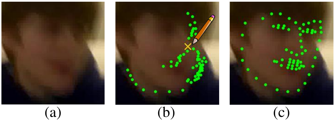
Recent work has suggested that interactive annotation can significantly improve the efficiency of labeling new datasets [\citeauthoryearLe et al.2012]. Our model can be used for this purpose through conditional prediction (Fig 11). Given evidence provided by a user (e.g., a single landmark click), compute the subset of pose-classes consistent with that evidence , and return the normalized softmax distribution over this subset:
| (10) |
In contrast, it is unclear how to incorporate such interactive evidence into regression-based methods such as CRMs.
We conduct an experiment to evaluate the impact of interactive annotation in Tab 3. In summary, by simply asking a user to annotate a single landmark (the nose) in each frame, one can reduce the error rate by 2-fold and correctly annotate 98.5% of the frames. By selecting an optimal landmark to label (through active learning on top of our probabilistic outputs), one can potentially reduce error by another factor of 2. Two demo videos can be found on the author’s website showing our interactive annotation in progress. Finally, when annotating a video dataset, similar approaches can be used to actively select both the key frame and key point that will be most informative (when combined with a HMM to obtain predictions for all other frames).
| Method | Failure rate (%) |
|---|---|
| No annotation (baseline) | 4.010 |
| 1-pt conditioning | 1.564 |
| Best 1-pt (upper bound) | 0.639 |
5 Conclusion
Though visual alignment is naturally cast as a regression problem, we reformulate it as a classification task. One significant advantage is that softmax classification networks naturally report back distributions, which can be used to reason about confidence, uncertainty, and condition on external evidence (provided by contextual constraints or an interactive user). Despite its simplicity, such a method is considerably more robust than prior work, producing state-of-the-art accuracy in challenging scenarios. We focus on the illustrative task of facial landmark alignment, demonstrating robust performance across large pose variation, severe occlusions and extreme illumination.
Acknowledgements: This research was supported in part by the National Science Foundation (NSF) under grant IIS-1618903, the Defense Advanced Research Projects Agency (DARPA) under Contract No. HR001117C0051, and the Office of the Director of National Intelligence (ODNI), Intelligence Advanced Research Projects Activity (IARPA), via IARPA R & D Contract No. D17PC00345. Additional support was provided by Google Research and the Intel Science and Technology Center for Visual Cloud Systems (ISTC-VCS). The views and conclusions contained herein are those of the authors and should not be interpreted as necessarily representing the official policies or endorsements, either expressed or implied, of ODNI, IARPA, or the U.S. Government. The U.S. Government is authorized to reproduce and distribute reprints for Governmental purposes notwithstanding any copyright annotation thereon.
References
- [\citeauthoryearBaltrusaitis, Robinson, and Morency2012] Baltrusaitis, T.; Robinson, P.; and Morency, L. P. 2012. 3D Constrained Local Model for rigid and non-rigid facial tracking. In CVPR, 2610–2617.
- [\citeauthoryearCao et al.2013] Cao, C.; Weng, Y.; Lin, S.; and Zhou, K. 2013. 3D Shape Regression for Real-time Facial Animation. In SIGGRAPH, volume 32.
- [\citeauthoryearChrysos et al.2017] Chrysos, G. G.; Antonakos, E.; Snape, P.; Asthana, A.; and Zafeiriou, S. 2017. A comprehensive performance evaluation of deformable face tracking ”in-the-wild”. IJCV.
- [\citeauthoryearCootes and Taylor1992] Cootes, T. F., and Taylor, C. J. 1992. Active Shape Models - ’Smart Snakes’. In BMVC, 266–275.
- [\citeauthoryearCootes and Taylor1993] Cootes, T. F., and Taylor, C. J. 1993. Active Shape Model Search using Local Grey-Level Models: A Quantitative Evaluation. In BMVC.
- [\citeauthoryearCootes, Edwards, and Taylor1998] Cootes, T.; Edwards, G.; and Taylor, C. 1998. Active appearance models. In ECCV.
- [\citeauthoryearDean et al.2013] Dean, T. L.; Ruzon, M. A.; Segal, M.; Shlens, J.; Vijayanarasimhan, S.; and Yagnik, J. 2013. Fast, accurate detection of 100, 000 object classes on a single machine. In CVPR.
- [\citeauthoryearDeng et al.2016] Deng, J.; Liu, Q.; Yang, J.; and Tao, D. 2016. M3 csr: Multi-view, multi-scale and multi-component cascade shape regression. Image Vision Comput. 47:19–26.
- [\citeauthoryearFan and Zhou2016] Fan, H., and Zhou, E. 2016. Approaching human level facial landmark localization by deep learning. Image Vision Comput. 47:27–35.
- [\citeauthoryearGirshick et al.2014] Girshick, R.; Donahue, J.; Darrell, T.; and Malik, J. 2014. Rich feature hierarchies for accurate object detection and semantic segmentation. In CVPR.
- [\citeauthoryearGross et al.2005] Gross, R.; Gross, R.; Matthews, I.; Matthews, I.; Baker, S.; and Baker, S. 2005. Generic vs. Person Specific Active Appearance Models. IVC.
- [\citeauthoryearHe et al.2016] He, K.; Zhang, X.; Ren, S.; and Sun, J. 2016. Deep residual learning for image recognition. CVPR.
- [\citeauthoryearJoulin et al.2016] Joulin, A.; van der Maaten, L.; Jabri, A.; and Vasilache, N. 2016. Learning visual features from large weakly supervised data. In ECCV.
- [\citeauthoryearKazemi and Josephine2014] Kazemi, V., and Josephine, S. 2014. One Millisecond Face Alignment with an Ensemble of Regression Trees. In CVPR, 1867–1874.
- [\citeauthoryearKemelmacher-Shlizerman et al.2016] Kemelmacher-Shlizerman, I.; Seitz, S. M.; Miller, D.; and Brossard, E. 2016. The megaface benchmark: 1 million faces for recognition at scale. 2016 IEEE Conference on Computer Vision and Pattern Recognition (CVPR) 4873–4882.
- [\citeauthoryearLe et al.2012] Le, V.; Brandt, J.; Lin, Z.; Bourdev, L.; and Huang, T. S. 2012. Interactive facial feature localization. In ECCV, 679–692. Springer.
- [\citeauthoryearLiu et al.2015] Liu, Z.; Luo, P.; Wang, X.; and Tang, X. 2015. Deep learning face attributes in the wild. In ICCV, 3730–3738.
- [\citeauthoryearMatthews and Baker2004] Matthews, I., and Baker, S. 2004. Active Appearance Models Revisited. IJCV 60(2):135–164.
- [\citeauthoryearPeng et al.2016] Peng, X.; Feris, R. S.; Wang, X.; and Metaxas, D. N. 2016. A recurrent encoder-decoder network for sequential face alignment. In ECCV.
- [\citeauthoryearRajamanoharan and Cootes2015] Rajamanoharan, G., and Cootes, T. F. 2015. Multi-view constrained local models for large head angle facial tracking. In ICCV Workshops.
- [\citeauthoryearRen et al.2014] Ren, S.; Cao, X.; Wei, Y.; and Sun, J. 2014. Face Alignment at 3000 FPS via Regressing Local Binary Features. In CVPR, 1685 – 1692.
- [\citeauthoryearRosch and Lloyd1978] Rosch, E., and Lloyd, B. B. 1978. Cognition and categorization, volume 1. Citeseer.
- [\citeauthoryearSagonas et al.2013] Sagonas, C.; Tzimiropoulos, G.; Zafeiriou, S.; and Pantic, M. 2013. 300 faces in-the-wild challenge: the first facial landmark localization challenge. In ICCV Workshops.
- [\citeauthoryearSagonas et al.2016] Sagonas, C.; Antonakos, E.; Tzimiropoulos, G.; Zafeiriou, S.; and Pantic, M. 2016. 300 faces in-the-wild challenge: database and results. Image Vision Comput. 47:3–18.
- [\citeauthoryearSánchez-Lozano et al.2016] Sánchez-Lozano, E.; Martínez, B.; Tzimiropoulos, G.; and Valstar, M. F. 2016. Cascaded continuous regression for real-time incremental face tracking. In ECCV.
- [\citeauthoryearSangineto2013] Sangineto, E. 2013. Pose and expression independent facial landmark localization using dense-surf and the hausdorff distance. PAMI 35(3):624–638.
- [\citeauthoryearSaragih, Lucey, and Cohn2011] Saragih, J. M.; Lucey, S.; and Cohn, J. F. 2011. Deformable model fitting by regularized landmark mean-shift. IJCV 91(2):200–215.
- [\citeauthoryearShen et al.2015] Shen, J.; Zafeiriou, S.; Chrysos, G. G.; Kossaifi, J.; Tzimiropoulos, G.; and Pantic, M. 2015. The first facial landmark tracking in-the-wild challenge: Benchmark and results. In ICCV Workshops, 1003–1011. IEEE.
- [\citeauthoryearTrigeorgis et al.2016] Trigeorgis, G.; Snape, P.; Nicolaou, M. A.; Antonakos, E.; and Zafeiriou, S. 2016. Mnemonic descent method: A recurrent process applied for end-to-end face alignment. In CVPR.
- [\citeauthoryearTzimiropoulos2015] Tzimiropoulos, G. 2015. Project-Out Cascaded Regression with an application to Face Alignment. In CVPR.
- [\citeauthoryearUricar and Franc2015] Uricar, M., and Franc, V. 2015. Real-time facial landmark tracking by tree-based deformable part model based detector. In ICCV-W, First Facial Landmark Tracking in-the-Wild Challenge and Workshop.
- [\citeauthoryearUricár, Franc, and Hlavác2015] Uricár, M.; Franc, V.; and Hlavác, V. 2015. Facial landmark tracking by tree-based deformable part model based detector. In ICCV Workshops.
- [\citeauthoryearWu and Ji2015] Wu, Y., and Ji, Q. 2015. Shape augmented regression method for face alignment. In ICCV Workshops.
- [\citeauthoryearXiao, Yan, and Kassim2015] Xiao, S.; Yan, S.; and Kassim, A. A. 2015. Facial landmark detection via progressive initialization. In ICCV Workshops.
- [\citeauthoryearXiong and De La Torre2013] Xiong, X., and De La Torre, F. 2013. Supervised descent method and its applications to face alignment. In CVPR, 532–539.
- [\citeauthoryearXiong and De La Torre2015] Xiong, X., and De La Torre, F. D. 2015. Global Supervised Descent Method. In CVPR.
- [\citeauthoryearYang and Patras2013] Yang, H., and Patras, I. 2013. Sieving Regression Forest Votes for Facial Feature Detection in the Wild. In ICCV, 1936–1943.
- [\citeauthoryearYang et al.2015] Yang, J.; Deng, J.; Zhang, K.; and Liu, Q. 2015. Facial shape tracking via spatio-temporal cascade shape regression. In ICCV Workshops.
- [\citeauthoryearYang et al.2016] Yang, S.; Luo, P.; Loy, C. C.; and Tang, X. 2016. Wider face: A face detection benchmark. In CVPR.
- [\citeauthoryearYu et al.2013] Yu, X.; Huang, J.; Zhang, S.; Yan, W.; and Metaxas, D. N. 2013. Pose-Free Facial Landmark Fitting via Optimized Part Mixtures and Cascaded Deformable Shape Model. In ICCV, 1944–1951.
- [\citeauthoryearZhang et al.2014] Zhang, Z.; Luo, P.; Loy, C. C.; and Tang, X. 2014. Facial landmark detection by deep multi-task learning. In ECCV.
- [\citeauthoryearZhang et al.2016a] Zhang, J.; Kan, M.; Shan, S.; and Chen, X. 2016a. Occlusion-free face alignment: Deep regression networks coupled with de-corrupt autoencoders. In CVPR.
- [\citeauthoryearZhang et al.2016b] Zhang, K.; Zhang, Z.; Li, Z.; and Qiao, Y. 2016b. Joint face detection and alignment using multitask cascaded convolutional networks. IEEE Signal Processing Letters 23(10):1499–1503.
- [\citeauthoryearZhu, Anguelov, and Ramanan2014] Zhu, X.; Anguelov, D.; and Ramanan, D. 2014. Capturing long-tail distributions of object subcategories. In CVPR, 915–922.
- [\citeauthoryearZhu et al.2015] Zhu, S.; Li, C.; Change, C.; and Tang, X. 2015. Face Alignment by Coarse-to-Fine Shape Searching. In CVPR.
- [\citeauthoryearZhu et al.2016] Zhu, X.; Lei, Z.; Liu, X.; Shi, H.; and Li, S. Z. 2016. Face alignment across large poses: A 3d solution. CVPR.