Unified Analysis and Optimization of D2D Communications in Cellular Networks Over Fading Channels
Abstract
This paper develops an innovative approach to the modeling and analysis of downlink cellular networks with device-to-device (DD) transmissions. The analytical embodiment of the signal-to-noise and-interference ratio (SINR) analysis in general fading channels is unified due to the H-transform theory, a taxonomy never considered before in stochastic geometry-based cellular network modeling and analysis. The proposed framework has the potential, due to versatility of the Fox’s H functions, of significantly simplifying the cumbersome analysis procedure and representation of DD and cellular coverage, while subsuming those previously derived for all the known simple and composite fading models. By harnessing its tractability, the developed statistical machinery is employed to launch an investigation into the optimal design of coexisting DD and cellular communications. We propose novel coverage-aware power control combined with opportunistic access control to maximize the area spectral efficiency (ASE) of DD communications. Simulation results substantiate performance gains achieved by the proposed optimization framework in terms of cellular communication coverage probability, average DD transmit power, and the ASE of DD communications under different fading models and link- and network-level dynamics. ††footnotetext: Work supported by the Discovery Grants and the CREATE PERSWADE programs of NSERC, and a Discovery Accelerator Supplement (DAS) Award from NSERC.
I Introduction
The recent sky-rocketing data demand has compelled both industry and regulatory bodies to come up with new paradigm-shifting technologies able to keep pace with such stringent requirements and cope with the massive connectivity characterizing future G networks. Currently being touted as a strong contender for G networks [1], [2], device-to-device (DD) communications allow direct communication between cellular mobiles, thus bypassing the network infrastructure, resulting in shorter transmission distances and improved data rates than traditional cellular networks.
In the past few years, DD-enabled networks have been actively studied by the research community. For example, in [3], it was shown that by allowing radio signals to be relayed by mobiles, DD communications can improve spectral efficiency and the coverage of conventional cellular networks. Additionally, DD has been applied to machine-to-machine (MM) communications [4] and proposed as a possible enabler of vehicle-to-vehicle (VV) applications [5]. More recent works [6]-[8] have modeled the user locations with PPP distributions and analytically tackled DD communication by harnessing the powerful stochastic geometry tools.
Notwithstanding these advances, computing the SINR in randomly deployed networks, namely DD-enabled cellular networks, has been successfully tractable only for fading channels and transmission schemes whose equivalent per-link power gains follow a Gamma distribution with integer shape parameter ([9] and references therein), while much work has been achieved on evaluating the performance of DD networks over Rayleigh fading channels [6]. Such particular fading distributions have very often limited legitimacy according to [10],[11], who argued that these fading models may fail to capture new and more realistic fading environments. This is particularly true as new communication technologies accommodating a wide range of usage scenarios with diverse link requirements are continuously being introduced and analyzed, for example, body-centric and millimeter-wave communications. Recently few works have been conducted to consider DD networks with general fading channels [12]-[15]. However, besides being channel-model-dependent, these works relied on series representation methods (e.g., infinite series in [14] and Laguerre polynomial series in [13],[15] ) thereby expressing the interference functionals as an infinite series of higher order derivative terms given by the Laplace transform of the interference power. These methods cannot lend themselves to closed-form expressions and, hence, require complex numerical evaluation.
For the successful coexistence of DD and cellular users, efficient interference management, e.g., through power or access control, is required. Recently, extensive research on power allocation strategies aiming to maximize the spectral efficiency of DD communication in random network models were studied and analyzed [16]-[18]. In [16], channel-aware power control algorithms aiming to maximize the DD sum rate are proposed and analyzed using stochastic geometry. In [17], SIR-aware access scheme based on the conditional coverage probability of DD underlaid cellular networks is proposed to increase the aggregate rate of DD links. Similarly, [18] proposes to enhance the sum rate of DD links by optimally finding groups and access probabilities. To the best of the authors’ knowledge, none of these works consider generalized fading channels when proposing access and power control schemes to accommodate multiple DD pairs underlaid in a cellular network. Yet, these works only focused on the simplistic Rayleigh fading.
In this paper, we focus on the design of access control and power allocation strategies for DD communication underlaying wireless networks under generalized fading conditions, an uncharted territory wherein the throughput potential of such networks remains unquantified. The contributions of this paper are as follows:
- •
We propose an analytical framework based on newly established tools from stochastic geometry analysis [9] to evaluate the cellular and DD SINR distributions in general fading conditions embodying the H-transform theory. We establish extremely useful results for the SINR and interference distributions never reported previously in the literature.
- •
We successfully unify our analysis framework in the sense that it can be applied for any fading channel whose envelope follows the form of , where stands for the Fox’s H function [19], e.g., Nakagami-, Weibull, or - and shadowed - to account for various small-scale fading effects such as LOS/NLOS (line-of-sight/non-LOS) conditions, multipath clustering, composite fading in specular or inhomogeneous radio propagation, and power imbalance between the in-phase and quadrature signal components.
- •
In order to guarantee the coverage probability of cellular users in a distributed manner, we derive the interference budget of a typical DD link, which represents the allowable transmit power level of DD transmitters. We formulate an optimization problem to find the access probability which maximizes the average area spectral efficiency utility of DD communication underlaying multiple cells subject to cellular coverage-aware power budget. The proposed opportunistic access requires only statistical CSI (channel state information), in contrast to the centralized resource allocation which requires full CSI, thereby inducing less delay in the network.
- •
We derive simple expressions for the optimal access probability and DD coverage-aware power budget based on an approximation of the DD coverage probability under both Nakagami- and Weibull fading channels. The developed machinery is prone to handle more comprehensive fading models, namely the shadowed -.
The remainder of this paper is organized as follows. We describe the system model in Section II. In Section III, we put forward the fading model-free statistical distribution of cellular and DD links in Section III, then we put forth the unifying H-transform analysis over the considered fading channels. We exploit in Section VI the developed statistical machinery to present the cellular coverage-aware power control and ASE of DD communications under different fading conditions. We present numerical results in Section V and conclude the paper in Section VII with some closing remarks.
II System Model
We envision a D2D-enabled cellular network model in which the locations of macro BSs (MBS) and DD users are distributed according to the independent homogeneous PPPs (HPPPs) and with intensities and , respectively. We assume (i) all users are served by the MBS from which they receive the strongest average power as their serving stations, which is equivalent to the nearest BS association criterion, and (ii) that a typical user is allowed to connect to a randomly selected DD transmitter (Tx). It is worth mentioning that the methodology of analysis to be presented later in this paper can be applied to different techniques pertaining to relaxing assumption (ii). It is worth mentioning here that the new analysis methodology proposed in this paper can be applied to different techniques pertaining to relaxing assumption (ii) by considering content availability [20], proximity [21] and clustering [22],[23]. Due to lack of space, we delegate for the sake of clarity these stand-alone extension materials to future works. We assume that all links between the transmitters (BS and DD Tx) to the typical user undergo distance dependent pathloss and small-scale fading. Then, the received power from the MBS/DD Tx located at , is given as where and are the transmit powers of the MBS and DD Txs, respectively, is the pathloss exponent and is an i.i.d. sequence of random variables modeling the channel power. The signal-to-interference plus noise ratio (SINR) at the location of the typical user when connecting to the nearest MBS () or to a randomly chosen DD Tx () can be expressed as
| (1) |
where, is the distance to the nearest MBS () and to the random DD Tx, respectively. The co-channel interference from other DD Txs or from other MBS are denoted by .
III Generalized SINR Analysis
In this section we derive the SINR distribution of a typical user in (i) a stand-alone cellular network in which only MBSs are available to provide coverage to any user, (ii) a stand-alone DD network in which only DD devices are available to provide coverage to any user. The obtained statistical machinery will be harnessed later to investigate underlaid DD networks.
Theorem 1: The SINR complementary cumulative distribution function (CCDF) of DD and cellular links, defined as for , is given by
| (5) | |||||
where , , , is the expectation with respect to the random variable , denotes the Fox-H function [24], [19] and
| (6) |
whereby and stand for the generalized hypergeometric [25, Eq. (9.14.1)] and the incomplete gamma [25, Eq.(8.310.1)] functions, respectively.
Proof: See Appendix A for details.
Theorem 1 demonstrates the general expressions of the Laplace transforms of and
as well as the DD and cellular SINR CCDFs without assuming any specific random channel gain and distance models11
1
In this paper,
the unbounded pathloss model is used due to its mathematical tractability. However more realistic models notably bounded
pathloss models (BPM) (, ) can be studied through the general SINR expression in Theorem 1..
Notice that in (5) is an integral transform that involves the Fox’s H-function as kernel, whence called H-transform. The H-transforms involving Fox’s H-functions as kernels were first suggested by Verma [26] with the help of -theory for integral transforms in the Lebesgue space [26]. So far, integral transforms, such as the classical Laplace, Mellin, and Hankel transforms have been used successfully in solving many problems pertaining to stochastic geometry modeling in cellular networks (cf.[6] and [9] and references therein). However, to the best of our knowledge, this paper is the first to introduce the Fox’s-H function and H-transforms to cellular network analysis. Since H-functions subsume most of the known special functions including Meijer’s G-functions [24], then by virtue of the essential so-called Mellin operation, involved in the Mellin transform of two H-functions, culminate in a H-function for any channel model with probability density function (PDF) .
A single H-variate PDF considers homogeneous radio propagation conditions and captures composite effects of multipath fading and shadowing, subsuming most of typical models such as Rayleigh, Nakagami-, Weibull, -Nakagami-, (generalized) -fading, and Weibull/gamma fading [27] as its special cases.
In contrast, to characterize specular and/or inhomogeneous environments, the multipath component consists of a strong LOS or specularly-reflected wave as well as unequal-power or correlated in-phase and quadrature scattered waves [10], [27], [28]. Another class of H-variate (degree-) PDF that is the product of an exponential function and a Fox’s H-function is used to account for specular or inhomogeneous radio propagation conditions including a variety of relevant models such as Rician, -, Rician/LOS gamma, and -/LOS gamma (or - shadowed) fading [10],[28] as special cases.
In this paper, we choose, however, to work with single H-variate fading PDFs to keep the presentation as compact as possible. Some other fading models that can still be considered within the framework of this paper are degree- H-variate fading models including the - and the shadowed -. We illustrate this fact in Appendix D.
Proposition 1 (Nakagami- Fading): The D2D and cellular SINR CCDFs over Nakagami- fading are given by
where , and
Proof: See Appendix B for details.
Definition 1: Consider the Fox’s-H function defined by [29, Eq. (1.1.1)]. It’s asymptotic expansion near is given by [29, Eq. (1.5.9)] as
| (16) |
where and is calulated as in [29, Eq. (1.5.10)].
Corollary 1 (Limits of Network Densification in Nakagami-m Fading) : The downlink SINR saturates past a certain network density as
| (17) |
Corollary 1 proves that at some point ultra-densification will no longer be able to deliver significant coverage gains. Although, some other works have also identified such fundamental scaling regime for network densification [6],[9], its network performance limits in terms of coverage have never been exactly quantified as in Corollary 1.
Due to potentially high density of devices, DD networks are overwhelmingly interference-limited. In this respect, the DD SIR distribution becomes
| (18) |
where follows form (84) when by resorting to [24, Eq.(2.19)] with . The analytical result in (18) applies to any spatial distribution of . It derives under Rayleigh distance, using [24, Eq.(2.19)], as
| (19) |
Proposition 2 (Weibull Fading): The Weibull fading channel accounts for the nonlinearity of a propagation medium with a physical fading parameters . When follows a Weibull distribution with parameters [27], then the SINR CCDFs of DD and cellular links are
where , and
| (26) |
Proof: See Appendix C for details.
Corollary 2 (Limits of Network Densification in Weibull Fading): For any SINR target , the cellular coverage probability in Weibull fading flattens out starting from some network density as
The DD SIR distribution is obtained from (91) as
where follows form applying [19, Eqs. 2.3] whereby .
Remark 1: The Rayleigh fading is a special case of (84) and (91) when and , respectively, thereby yielding
with
| (38) |
where follows after recognizing that , when stands for the DiracDelta function, i.e., . The coverage formulas in (III) matches the well-known major results for Rayleigh fading obtained in [6, Theorem 1] with the valuable add-on of being in closed-form.
IV Area Spectral Efficiency Optimization
Hereafter, we consider a cellular network underlaid with DD Txs. We assume an ALOHA-type channel access for both DD and cellular Txs with probability and , respectively. Then, the set of active MBS/DD Txs also forms a HPPP with density where . We assume that each cellular transmitter has its intended receiver at a fixed distance in a random direction. Similarly, each DD receiver is located at distance from its corresponding transmitter.
The ASE, often referred to as network throughput, is a measure of the number of users that can be simultaneously supported by a limited radio frequency bandwidth per unit area.
Definition 2: In DD-underlaid cellular networks, the ASE of DD communications can be expressed as [17]
| (39) |
where is the mean of the DD coverage probability (previously derived in Section III), denotes the effective DD link density without any inactive DD link, and is the access probability.
In what follows, capitalizing on the statistical framework developed in section III, we present quality-based power control strategies for DD communications under both Nakagami- and Weibull fading channels aiming to reduce the interference caused by DD Txs and to maximize the ASE of DD communications.
IV-A Cellular Coverage Probability-Aware Power Control
Consider an arbitrary cellular transmitter and its associated receiver at distance . We are interested in investigating the joint effect of the interference coming from the surrounding BS and the DD Txs on the downlink coverage probability while ignoring the noise by assuming . Therefore the SIR at the cellular receiver is expressed as
| (40) | |||||
where is the ratio of the transmit powers of the DD. Let be the operator-specified cellular success probability threshold. The maximum transmit power for DD Txs is obtained by solving the following optimization problem:
| (41) | |||||
where for any , the cellular coverage probability, conditioned on , can be expressed over general fading based on (40) and employing (5) as
| (42) | |||||
where is a function of only the fading parameters as previously shown in (84) and (91). Moreover, assuming that the distance-based association policy imposes no constraint on the location of interfering MBSs to the probe receiver, we have
| (43) |
IV-A1 DD Power Control Under Nakagami- Fading
In this section, we assume that all links experience Nakagami- flat fading channel. The fading severity of the Nakagami- channel is captured by the parameter for all links originating from the DD transmitters, while the fading severity of the cellular communication and interference links is captured by the parameter .
Proposition 3: The maximum DD transmit power can be expressed under Nakagami- fading as
| (44) | |||||
which acts as an average individual interference budget of each DD Tx to guarantee the coverage probability of cellular users, where , and is the principal branch of the Lambert function [25].
Proof: The cellular coverage probability under Nakagami- fading follows from (42) as
| (48) | |||||
Definition 3: Consider the Fox’s-H function defined by [29, Eq. (1.1.1)]. Its asymptotic expansion near when is given by [29, Eq. (1.7.14)]
| (49) |
where , , and are constants defined in [29, Eq. (1.1.8)], [29, Eq. (1.1.9)], and [29, Eq. (1.1.10)], respectively. Then follows after recognizing that , , . Thus, the problem in (41) can be solved by (48)(b)-. The latter is a homogeneous equation, which is solvable, thereby yielding the desired result after some mathematical manipulations.
IV-A2 DD Power Control Under Weibull Fading
In this section, we assume that all links experience Weibull flat fading channel. Specifically, the cellular interfering link suffers from the Weibull () fading and the DD interference link experiences the Weibull () fading.
Proposition 4: The cellular success probability-aware power control under Weibull fading yields
| (50) |
where , , , and .
Proof: The cellular coverage probability under Weibull fading follows from (42) as
| (54) | |||||
where follows from applying (91) whereby is given in (92) and . Moreover follows from resorting to (49). Subsequently, by solving (54)(b)-, we get (50) after some mathematical manipulations.
In reality, the individual interference budgets in (44) and (50) may be calculated and broadcast by MBSs to each DD Tx at the initial stage. In order to use the licensed spectrum, each DD Tx must obey the individual interference budget in its power allocation stage. Note that our problem formulation is based on the distributed power control framework where cellular users and DD Txs do not need to share location or channel state, which implies that the individual interference budget in (44) and (50) do not require the instantaneous CSI which is in fact difficult to get accurately especially upon high mobility of cellular and DD users. Under the proposed distributed power allocation framework, a DD Tx selects its transmit power based solely on the knowledge of the cross-tier communication distance , the users and MBS spatial density, and the joint effect of path loss and fading. Compared to most existing schemes for DD power control that are based on the real-time CSI to mitigate interference ([16] and references therein), the proposed power control framework, being statistically featured, does not burden the network latency.
In particular, from (44) and (50) we prove that the cellular user coverage probability guarantee can be distributively satisfied regardless of whether the DD transmitters adapt their transmit power or access probability. In other words, DD users can tune either of these two parameters representing an interference budget that each DD pair may not exceed toward the cellular users.
IV-B DD ASE-Aware Access Probability
In densely deployed DD networks, both DD to cellular and inter-DD interferences would be very high. As a result, the cellular coverage probability threshold may not be guaranteed, even under individual DD interference budget, especially when the target cellular SIR threshold is high. Hereafter, instead of allowing all DD transmitters to access the channels, a part of DD pairs cannot access the network to decrease interferences. Hence we propose to extend the cellular coverage probability-aware power control by integrating it with opportunistic access control to maximize the area spectral efficiency of DD communications while decreasing both inter-DD and cross-tier interferences.
After obeying to the individual interference budget in its power allocation stage, each DD Tx maximizes its ASE utility by optimizing the access probability . We formulate the individual access-aware design problem of DD Tx as
| (55) |
where is defined in (39) with maximum permissible transmit power for an arbitrary DD user at a particular MAP obtained from (44), and is the SIR coverage probability of an arbitrary DD link obtained as
| (56) | |||||
IV-B1 DD ASE under Nakagami- Fading
Under Nakagami- fading, and conditioned on , the SIR coverage probability of an arbitrary DD link under transmit power adaptation (i.e., considering (44)) follows from applying (56) while considering (18) as
| (60) | |||||
where is the maximum DD transmit power of DD Tx identified by cellular success probability-aware power control,
| (61) |
and follows from applying the algebraic
asymptotic expansions of the Fox’s-H function in (49) with several mathematical manipulations.
Based on (64), (55) can be transformed further to
| (62) |
where .
Proposition 5: The optimal access probability under Nakagami- fading verifies
| (63) |
and is easily decided, after some manipulations, by
| (64) |
The DD area spectral efficiency when operating at (, ) can be quantified under Nakagami- fading as
| (65) |
where .
IV-B2 DD ASE under Weibull Fading
The area spectral efficiency of DD underlay cellular networks under Weibull fading and cellular success probability-aware power control (i.e., considering (50)) can be expressed as
| (66) |
where , , and
| (67) |
Proof: Following the same rationale to obtain (64), while considering (50), yield the success probability of DD underlay network under Weibull fading with maximum permissible transmit power. Plugging the obtained result into (39) completes the proof.
Proposition 6: The optimal access probability () which maximizes the area spectral efficiency for DD underlay network under cellular success probability-aware power control operating over Weibull fading verifies
| (68) |
obtained from the maximization of the area spectral efficiency in (66), thereby yielding
| (69) |
Plugging into (66) yields the DD underlay network ASE with cellular success probability-aware power control and opportunistic access control under Weibull fading as
| (70) |
Note that both the optimal access probability and ASE are inversely proportional to the DD link distance . That is implying that a DD Tx with a short communication distance has a higher access probability than a DD transmitter with a larger communication distance, because it has a potentially higher SIR. We also notice that is inversely related to the density of DD users (). Notice that in many studies that intrinsically rely on the optimality of access or power against density adaptation [30], a similar behavior was noticed. However, in this paper, we show that both the access and transmit power adaptations by themselves are sub-optimal. To overpass such suboptimality, we extend cellular success probability-aware power control by integrating it with opportunistic access control to maximize the area spectral efficiency of DD communications.
V Numerical And Simulation Results
In this section, numerical examples are shown to substantiate the accuracy of the new unified mathematical framework and to explore from our new analysis the effects of both the link- and network- level dynamics22 2 Link-level dynamics correspond to the uncertainty experienced due to multi-path propagation and topological randomness, while network-level dynamics are shaped by medium access control, device/BS density, etc. on the ASE of the underlay DD network.


Fig. 1 shows the ASE of the DD underlay network under Nakagami- fading as a function of the DD transmit power. We can notice that DD transmitters can increase their transmit power to improve DD receivers’ ASE up to a maximum value beyond which the operation becomes unfeasible due to the bound enforced by the cellular network. Fig. 1 also shows that transmit power and access probability play a dual role. Indeed, an increase in the operational access probability inflicts a higher co-channel interference to the cellular user and, hence, a more stringent operational constraint by a reduction in the individual DD interference budget (the maximum permissible transmit power) and thereby of the ASE. Hence the gain obtained due to an increase in the simultaneous transmissions may vanish because of the reduction in the success probabilities of the individual links. This indicates that there may exist an optimal operational point where the reduction in the link coverage can be balanced by increasing the number of concurrent transmissions.
Fig. 2 plots the ASE of the DD underlay network under Nakagami- fading as a function of the DD mean access probability. We observe that the maximum permissible density of the active DD transmitters is bounded due to the cellular user’s coverage constraint, thereby consolidating the trends of Fig. 1. Fig. 2 further investigates the impact of cellular and DD channel fading severities and user densities on the ASE. For almost equally densely deployed cellular and DD networks, DD performance is governed by the fading severity rather than . In this case, cellular users employ higher transmit power thereby bounding the DD underlay network performance due to the inflicted cellular interference. The dominant fading severity parameter is reversed when which is hardly surprising because the increased density limits the DD network’s performance by its own co-channel interference. In brief, Fig. 2 stipulates that the ASE of DD networks is jointly dependent on the density of users and the propagation conditions.
Fig. 3 depicts the ASE of the DD underlay network as a function of the DD mean access probability under Weibull fading. As observed in Fig. 3 the ASE is strongly coupled with the fading severity of the propagation channel. For a DD network more densely deployed than the cellular network (), the fading severity plays a more important role than . Hence, the attainable ASE is dramatically reduced when the fading severity of inter-tier DD communication and cross-tier interference channel is reduced. In fact, a reduced power budget due to an increased fading parameter (small fading severity) outweighs the performance gain due to better propagation conditions for the communication link.
Fig. 4 plots the ASE in Weibull fading for several different values of against the DD mean access probability. We observe that reducing enlarges the DD operational region in terms of access probability at smaller ASE values. This is in fact due to less cross-iter interference with a reduced signal power at the DD receiver. Consequently, although a smaller may increase the access probability limit, the attained performance may deteriorate due to the reduction of the overall ASE.
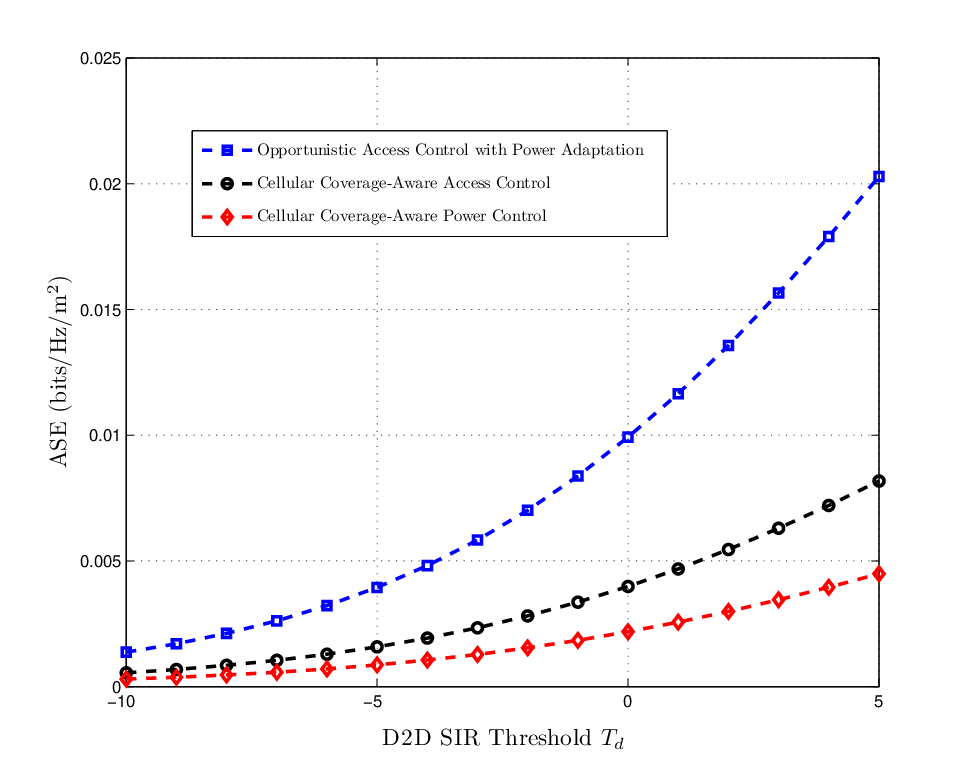
Fig. 5, compares the performance of the cellular coverage-aware power or access control and the opportunistic access control combined with cellular coverage-aware power control. We notice that the latter scheme greatly improves the ASE of DD communications comparing to sole adaptation of a single degree of freedom (transmit power or access probability) with an arbitrary selection of the other resulting in a sub-optimal performance. On the other hand, the maximum ASE under cellular coverage-aware access control is higher than the one attained with power control. However, the maximum ASE is bounded by a wall due to the primary user’s QoS requirements.
VI CONCLUSION
In this paper, we developed a new methodology for modeling and analyzing DD-enabled cellular networks over general fading channels that relies on the H-transform theory. This methodology subsumes most known fading models and more importantly enables the unified analysis for the SINR distribution of DD communications. This framework is traditionally intractable due to the model-dependent limit on the distribution of the SINR in previous derivations. We build upon the developed statistical machinery to formulate an optimization scheme for DD networks in terms of SIR and spectral efficiency. This scheme combines power control that is aware of cellular coverage probability with opportunistic access control. That is to reduce the interference caused by DD communications and maximize the area spectral efficiency of DD communications. We show that the optimal proportion and transmit power of active devices can be easily obtained by simple fading model-specific formulas, thereby serving as a useful tool for network designers to better understand and fine-tune the performance of DD-enabled cellular networks.
VII Appendix
VII-A Proof of Theorem 1:
The SINR CCDF may be retrieved from its Laplace transform as
| (71) |
where denotes the SINR moment generating function recently derived in [9, Theorem 1]. Hence it follows that
| (72) |
where denotes the Laplace transform of the aggregate interference, and , where is the Bessel function of the second kind [25, Eq. (8.402)] and stands for the inverse Laplace transform. Resorting to [19, Eq. (1.127) ] and [19, Eq. (2.21)], we get
| (73) |
Plugging (73) into (72) and carrying out the change of variable relabeling as yield
| (77) | |||||
The Laplace transform of the interference at the cellular receiver, , is evaluated as follows
| (78) |
where
| (79) | |||||
and the PGFL of a HPPP with intensity function is used in the first equality, is applied in , and follows from letting and applying .
VII-B Proof of Proposition 1:
Let be a random variable with put in the form of a single H-variate [19, Eq. (1.125)], then applying [25, Eqs. (7.813), (9.31.5)] yields after some manipulations. On the other hand, is obtained from (6) while and follows from (6) after applying [25, Eq. (7.522.9) ]. Plugging all these results in (5) and (6) yields
| (84) | |||||
where
We assume that the distance between a typical user and its associated MBS (cellular link) or DD helper (DD link) follows a Rayleigh distribution, i.e. [6]. Hence, substituting for cellular and DD users in (84) and resorting to [19, Eq. (2.3)] yield (III) after some manipulations.
VII-C Proof of Proposition 2:
The proof follows from (5) with and applying [19, Eqs. (2.3), (1.56)]. Besides, follows by resorting to . On the other hand, recalling that and applying [19, Eqs. (2.3)] yield after some manipulations using the Fox-H function properties in [24, Eqs. (1.2.3), (1.2.4)]. Plugging all these results in (5) and (6) yields
| (91) | |||||
where
| (92) |
Finally, substituting for cellular and DD users and proceeding as before completes the proof.
VII-D - and Shadowed - As Special Cases of the Degree-2 Fox’s H-Function Fading Model
The - distribution, first introduced in [10], can be regarded as a generalization of the classic Rician fading model for LOS scenarios. Let be a random variable statistically following a - distribution [31] with mean and non-negative real shape parameters , and , with
| (93) |
where stands for the modified Bessel function of the first kind of order [25, Eq. (8.431.1)]. Recognizing that [19, A.7 ]
| (94) |
where , then from (5) it follows that in - fading
| (98) | |||||
The last H-transform is known as the Laplace transform of two Fox’s-H function given by [24, Eq. (2.6.2)] as
where denotes the generalized Fox’s H-function of two variables [32, Eq. (1.1)] and it reduces with the help of [24, Eq. (2.3.1)] to the generalized Meijer’s G-function of two variables. Recalling that under - fading [13, Eq. (10)], thereby yielding as in (109). On the other hand is obtained from (6) using where then applying [33, Eq. (27)] yield
| (103) | |||||
where stands for the Humbert function of the first kind [33, Eq. (2)]. Plugging all these resulst into (5) yields the DD and cellular CCDFs as
| (108) | |||||
where , and is obtained as
| (109) |
where with , and is the generalized Meijer’s G-function of two variables [26].
In interference-limited - environment, the SIR CCDF of DD links is obtained as
where follows from substituting by its expression in (109) after recognizing the Fox’s-H representation of the exponential function [24, Eq. (1.7.2)] and employing [24, Eq. (2.11)]. Moreover, . Notice that the - includes the Rayleigh , Nakagami- , and Rician fading models as special cases, where is the Rician factor.
In shadowed - distribution the dominant signal components are subject to Nakagami- shadowing with pdf [28, Table I]
| (121) | |||||
where denotes the confluent hypergeometric function of [25, Eq. (13.1.2)]. Recalling that
| (122) |
then the DD and cellular SINR CCDFs follow along the same line of (108) as
| (127) | |||||
where . Moreover in (127), is obtained as
| (128) |
where follows after recognizing that [13, Eq. (10)] thereby yielding . On the other hand, is obtained from (6) along the same line of (109) while considering the following integral form
| (129) | |||||
where stands for the Appell’s hypergeometric function of the second kind [34, Eq. (27)].
We assume that the communication is interference limited and hence thermal noise is negligible. Then the coverage of DD communication in - shadowed fading is obtained as
where .
References
- [1] M. N. Tehrani, M. Uysal, and H. Yanikomeroglu, ”Device-to-device communication in 5G cellular networks: Challenges, solutions, and future directions,” IEEE Commun. Mag., vol. 52, no. 5, pp. 86-92, May 2014.
- [2] B. Bangerter, S. Talwar, R. Arefi, and K. Stewart, ”Networks and devices for the 5G era,” IEEE Commun. Mag., vol. 52, no. 2, pp. 90-96, 2014.
- [3] K. Doppler, M. Rinne, C. Wijting, C. B. Ribeiro, and K. Hugl, ”Device-to-device communication as an underlay to LTE-advanced networks,” IEEE Commun. Mag., vol. 47, no. 12, pp. 42-49, Dec. 2009.
- [4] S.-Y. Lien, K.-C. Chen, and Y. Lin, ”Toward ubiquitous massive accesses in 3GPP machine-to-machine communications,” IEEE Commun. Mag., vol. 49, no. 4, pp. 66-74, Apr. 2011.
- [5] H. Ilhan, M. Uysal, and I. Altunbas, ”Cooperative diversity for intervehicular communication: Performance analysis and optimization,” IEEE Trans. Veh. Technol., vol. 58, no. 7, pp. 3301-3310, Sep. 2009.
- [6] X. Lin, J. G. Andrews, and A. Ghosh, ”Spectrum sharing for device-to-device communication in cellular networks,” IEEE Trans. Wirel. Commun., vol. 13, no. 12, pp. 1-31, Dec. 2014.
- [7] G. George, R. K. Mungara, and A. Lozano, ”An analytical framework for device-to-device communication in cellular networks,” IEEE Trans. Wireless Commun., vol. 14, no. 11, pp. 6297-6310, Nov. 2015.
- [8] H. ElSawy, E. Hossain, and M. S. Alouini, ”Analytical modeling of mode selection and power control for underlay D2D communication in cellular networks,” IEEE Trans. Commun., vol. 62, no. 11, pp. 4147-4161, Nov. 2014.
- [9] I. Trigui, S. Affes, and B. Liang, ”Unified stochastic geometry modeling and analysis of cellular networks in LOS/NLOS and shadowed fading,” IEEE Trans. Commun., vol. 5, no. 99, pp. 1-16, July 2017.
- [10] M. D. Yacoub, ”The - distribution and the - distribution,” IEEE Antennas Propag. Mag., vol. 49, no. 1, pp. 68-81, Feb. 2007.
- [11] N. Beaulieu and X. Jiandong, ”A novel fading model for channels with multiple dominant specular components,” IEEE Wireless Commun. Lett., vol. 4, no. 1, pp. 54-57, Feb. 2015.
- [12] M. Peng, Y. Li, T. Q. S. Quek, and C. Wang, ”Device-to-device underlaid cellular networks under Rician fading channels,” IEEE Trans. Wirel. Commun., vol. 13, no. 8, pp. 4247-4259, Aug. 2014.
- [13] Y. J. Chun, S. L. Cotton, H. S. Dhillon, F. J. Lopez-Martinez, J. F. Paris, and S. Ki Yoo ”A Comprehensive analysis of 5G heterogeneous cellular systems operating over - shadowed fading channels”, CoRR, vol. arXiv:1609.09389, 2016. [Online].
- [14] S. Parthasarathy and R. K. Ganti, ”Coverage analysis in downlink poisson cellular network with - shadowed fading,” IEEE Wireless Commun. Lett., vol. 6, no. 1, Feb. 2017.
- [15] Y. J. Chun, S. L. Cotton, H. S. Dhillon, A. Ghrayeb, and M. O. Hasna, ”A stochastic geometric analysis of device-to-device communications operating over generalized fading channels,” IEEE Trans. Wireless Commun., vol. 16, no. 7, pp. 4151-4165, Jul. 2017
- [16] N. Lee, X. Lin, J. G. Andrews, and R. W. Heath, ”Power control for DD underlaid cellular networks: Modeling, algorithms, and analysis,” IEEE J. Sel. Areas Commun., vol. 33, no. 1, pp. 1-13, Jan. 2015.
- [17] Z. Chen and M. Kountouris, ”Distributed SIR-aware opportunistic access control for D2D underlaid cellular networks,” in Proc. IEEE Globecom, Austin, TX, USA, pp. 1540-1545, Dec. 2014.
- [18] J. Park and J. H. Lee, ”Semi-distributed spectrum access to enhance throughput for underlay device-to-device communications”, IEEE Trans. Commun., vol. 65, no. 10, Oct. 2017.
- [19] M. Mathai, R. K. Saxena, and H. J. Haubold, The H-function: Theory and Applications, Springer, New York, 2010.
- [20] M. Afshang, H. S. Dhillon, and P. H. J. Chong, ”Fundamentals of clustercentric content placement in cache-enabled device-to-device networks,” IEEE Trans. Commun., vol. 64, no. 6, pp. 2511-2526, Jun. 2016.
- [21] M. Afshang, H. S. Dhillon, and P. H. J. Chong, ”k-closest coverage probability and area spectral efficiency in clustered D2D networks,” in Proc. IEEE Int. Conf. Commun. (ICC), Kuala Lumpur, Malaysia, May 2016.
- [22] C. Saha, M. Afshang, H. S. Dhillon, ”3GPP-inspired HetNet model using poisson cluster process: sum-product functionals and downlink coverage”, IEEE Trans. Commun., vol. 65, no. 10, Dec. 2017.
- [23] M. Afshang, H. S. Dhillon, and P. H. J. Chong, ”Modeling and performance analysis of clustered device-to-device networks,” IEEE Trans. Wireless Commun., vol. 15, no. 7, July 2016.
- [24] A. M. Mathai and R. K. Saxena, The -Function With Applications in Statistics and Other Disciplines. New Delhi, India: Wiley Eastern, 1978.
- [25] I. S. Gradshteyn and I. M. Ryzhik, Table of Integrals, Series and Products, 5th ed., Academic Publisher, 1994.
- [26] R. U. Verma, ”On some integrals involving Meijer’s G-fucntion of two variables”, Proc. Nat. Inst. Sci. India, vol. 39, Jan. 1966.
- [27] M. K. Simon and M.-S. Alouini, Digital Communication over Fading Channels. Wiley-Interscience, 2005, vol. 95.
- [28] J. F. Paris, ”Statistical characterization of - shadowed fading,” IEEE Trans. Veh. Technol., vol.63, no. 2, pp. 518-526, Feb. 2014.
- [29] A. Kilbas and M. Saigo, H-Transforms: Theory and Applications, CRC Press, 2004.
- [30] H. Kobayashi, Y. Onozato, and D. Huynh, ”An approximate method for design and analysis of an ALOHA system,” IEEE Trans. Commun., vol. 25, no. 1, pp. 148-157, 1977.
- [31] L. Moreno-Pozas, F. J. Lopez-Martinez, J. F. Paris, and E. Martos-Naya, ”The - shadowed fading model: Unifying the - and - distributions,” IEEE Trans. Veh. Technol., vol. 65, no. 12, pp. 9630-9341, Dec. 2016.
- [32] P. Mittal and K. Gupta, ”An integral involving generalized function of two variables”, Proc. Ind. Acad. Sci., vol. 75, no. 3, pp. 117–123, 1972.
- [33] Yu. A. Brychkova and N. Saad, ”On some formulas for the Appell function Integral Transforms and Special Functions, vol. 25, no. 2, pp. 111-123, 2014.
- [34] S. B. Opps, N. Saad, and H.M. Srivastava, ”Some reduction and transformation formulas for the Appell hypergeometric function ” Journal of Mathematical Analysis and Applications, vol. 302, pp. 180-195, Feb. 2005.