Resilience of scrambling measurements

Brian Swingle Affiliation: Condensed Matter Theory Center, Maryland Center for Fundamental Physics, Joint Center for Quantum Information and Computer Science, and Department of Physics, University of Maryland, College Park, MD 20742, USA Affiliation: Kavli Institute for Theoretical Physics, University of California, Santa Barbara, CA 93106, USA Nicole Yunger Halpern Note: E-mail: nicoleyh@caltech.edu Affiliation: Institute for Quantum Information and Matter, Caltech, Pasadena, CA 91125, USA Affiliation: Kavli Institute for Theoretical Physics, University of California, Santa Barbara, CA 93106, USA

Abstract

Most experimental protocols for measuring scrambling require time evolution with a Hamiltonian and with the Hamiltonian’s negative counterpart (backwards time evolution). Engineering controllable quantum many-body systems for which such forward and backward evolution is possible is a significant experimental challenge. Furthermore, if the system of interest is quantum-chaotic, one might worry that any small errors in the time reversal will be rapidly amplified, obscuring the physics of scrambling. This paper undermines this expectation: We exhibit a renormalization protocol that extracts nearly ideal out-of-time-ordered-correlator measurements from imperfect experimental measurements. We analytically and numerically demonstrate the protocol’s effectiveness, up to the scrambling time, in a variety of models and for sizable imperfections. The scheme extends to errors from decoherence by an environment.

I Introduction

Quantum information scrambles when it spreads over all the degrees of freedom of a quantum many-body system, becoming inaccessible to few-body probes [1, 2, 3]. In a recent spate of theoretical activity, scrambling has been related to early-time signatures of quantum chaos [4, 5, 6, 7], to the scattering of high-energy quanta near a black-hole horizon [8, 9], to bounds on the propagation of quantum information [10], to quasiprobabilities (nonclassical generalizations of probabilities) [11, 12], to thermodynamic fluctuation relations [11, 13, 14], to Schwinger-Keldysh path integrals [15, 16, 17, 18], to quantum channels [19], to unitary $k$ -designs [20, 21, 22], and to much else. On the experimental side, many proposals for observing scrambling now exist [23, 24, 25, 26, 11, 12, 27, 13, 28], and at least four early experiments have been performed [29, 30, 31, 32].

Central to these developments is a physical quantity called the out-of-time-ordered correlator (OTOC). Consider a quantum many-body system governed by a Hamiltonian $H$ that generates the time-evolution unitary $U$ . Let $\rho$ denote a state of the system, e.g., a thermal state $e^{-\beta H}/Z$ , for some inverse temperature $\beta$ and a partition function $Z$ . Let $W$ and $V$ denote Hermitian or unitary operators defined on the system’s Hilbert space. $W$ evolves as $W_{t}:=U^{\dagger}WU$ in the Heisenberg picture. The OTOC is defined as

\displaystyle F_{t}:=\langle W^{\dagger}_{t}V^{\dagger}W_{t}V\rangle\equiv{\rm Tr}(W^{\dagger}_{t}V^{\dagger}W_{t}V\rho)\,.

(1)

The operators’ ordering lends the OTOC its name. We can grasp one significance of $F_{t}$ by assuming that $\rho=\lvert\psi\rangle\!\langle\psi\rvert$ is pure, $V$ is unitary, and $W$ is Hermitian. Consider two protocols that differ just via an order of operations: (i) Prepare $\lvert\psi\rangle$ , perturb the system with $V$ , evolve the system forward in time with $U$ , measure $W$ , and evolve the system backward with $U^{\dagger}$ . This protocol prepares $W_{t}V\lvert\psi\rangle=:\lvert\psi^{\prime}\rangle$ . (ii) Prepare $\lvert\psi\rangle$ , evolve the system forward, measure $W$ , evolve the system backward, and measure $V$ . This protocol prepares $VW_{t}\lvert\psi\rangle=:\lvert\psi^{\prime\prime}\rangle$ . The discrepancy between the protocols imprints on the overlap $|\langle\psi^{\prime\prime}|\psi^{\prime}\rangle|=|F_{t}|$ .

As this forward-and-backward explanation suggests, OTOCs resemble the well-known Loschmidt echo in spirit (see [33, 34] for a review). Like observations of the echo, most OTOC-measurement proposals require the experimenter to effectively reverse the flow of time. Unfortunately, effective time reversal is typically experimentally challenging. No general method for circumventing this difficulty is known. OTOC-measurement protocols that do not require time reversal suffer from other limitations that likely preclude the study of large systems. Nevertheless, progress in the control of atoms, molecules, ions, and photons has brought experimental measurements of OTOCs and scrambling seemingly within reach [29, 30, 31, 32].

One may wonder if the difficulty of precisely reversing time’s flow is more than technical. Perhaps, for sufficiently large, complex, chaotic quantum many-body systems, small imperfections in the time-reversal procedure will always be amplified and obscure the physics of interest. We believe that a fault-tolerant quantum computer could implement the time reversal with satisfactory accuracy. But do we need such a resource?

We argue that these concerns, while reasonable, are not borne out in practice. We show how a simple renormalization procedure can be used to extract OTOCs’ early-time dynamics. The renormalization requires only experimentally measurable quantities. The dynamics of chaotic quantum many-body systems can be recovered.

We offer theoretical arguments, and numerical and analytical evidence, for the following claim: The ideal OTOC’s essential physics can, up to the scrambling time, be extracted from imperfect measurements in which the forward and backward time evolutions differ by $10\%$ or more from their ideal forms: Each implemented Hamiltonian differs from the ideal Hamiltonian $H$ by terms that carry an overall scale factor $\varepsilon\leq 0.1$ . This resilience is quite universal: The system can exhibit strong chaos or integrability. The interactions can be local or nonlocal. Our result holds even when imperfections vary from experimental run to experimental run.

Detailed numerical studies of a one-dimensional quantum Ising chain support our general derivations. So does an analytical calculation with a strongly chaotic model dual to a black hole. The renormalization scheme works here if the time $t$ for which the system evolves forward differs from the time $t^{\prime\prime}$ for which the system evolves backward. Though Hamiltonian errors motivate much of this paper, also decoherence by the environment threatens OTOC measurements. The renormalization scheme helps combat decoherence, as we show with numerical simulations and tailored analytical calculations.

Our physical picture of this resilience phenomenon is that the imperfect OTOC contains two pieces of physics. One piece consists of the growth of operators, and the spreading of information, characteristic of scrambling. One piece consists of the decay of fidelity due to mismatched forward and backward time evolutions (similar to the traditional Loschmidt echo). We claim that these two pieces of physics can be effectively separated, and that the second piece can be cleaned off from the first, until the scrambling time, through the use of only experimentally measurable data.

We focus on two scrambling protocols, the interferometric protocol [23] and the weak-measurement protocol [11, 12]. But we expect our results to extend to other OTOC measurement schemes. The paper is structured as follows: Section II concerns the interferometric scheme. Section III concerns the weak measurement scheme. Section IV concerns environmental decoherence (for both schemes). Section V shows our scheme’s efficacy in a strongly chaotic holographic model plagued by unequal-time evolutions, via analytical calculation. Section VI concludes with future directions and open questions.

II Example #1: Interferometer

The interferometric scheme for measuring the OTOC was introduced in [23]. The set-up and protocol are reviewed in Sec. II.1. The protocol can suffer from Hamiltonian errors detailed in Sec. II.2. The renormalization scheme mitigates those errors. We motivate the renormalization mathematically in Sec. II.3. Section II.4 supports the scheme with numerical simulations of the power-law quantum Ising model.

II.1 Set-up and protocol for the interferometer

Let ${\mathcal{S}}$ denote the system of interest, associated with a Hilbert space $\mathcal{H}$ . We illustrate with a chain of $n$ qubits (spin- $\frac{1}{2}$ degrees of freedom). Let $\sigma^{\alpha}_{j}$ denote the $\alpha=x,y,z$ component of the $j^{\rm th}$ site’s spin. The $+1$ and $-1$ eigenstates of $\sigma^{z}$ are denoted by $\lvert 0\rangle$ and $\lvert 1\rangle$ .

A Hamiltonian $H$ determines the system’s natural dynamics. $H$ generates the time-evolution operator $U:=e^{-iHt}$ .

Let $W$ and $V$ denote local unitaries. Unitaries that nontrivially transform only faraway subsystems reflect scrambling. For example, $W$ can manifest as the first qubit’s Pauli- $z$ operator: $W=\sigma^{z}_{1}\otimes\mathbbm{1}^{\otimes(n-1)}$ . $V$ can manifest as the final qubit’s Pauli- $x$ operator: $V=\mathbbm{1}^{\otimes(n-1)}\otimes\sigma^{x}_{n}$ . In the Heisenberg Picture, $W$ evolves as $W_{t}:=U^{\dagger}WU$ .

For simplicity, we focus on pure states $\lvert\psi\rangle\in\mathcal{H}$ . The interferometric scheme, however, generalizes to arbitrary $\rho\in\mathcal{D}(\mathcal{H})$ , the set of density operators (trace-one linear positive-semidefinite operators) defined on $\mathcal{H}$ . The OTOC has the form $F_{t}=\langle\psi|W^{\dagger}_{t}V^{\dagger}W_{t}V|\psi\rangle$ . Figure 1 illustrates the interferometric protocol. The system-and-control composite ${\mathcal{S}}{\mathcal{C}}$ ends a perfect trial in the state

\displaystyle\lvert\Psi^{\prime}\rangle

\displaystyle:=\frac{1}{\sqrt{2}}[VW_{t}\lvert\psi\rangle\otimes\lvert 0\rangle+W_{t}V\lvert\psi\rangle\otimes\lvert 1\rangle]\,.

(2)

Refer to caption — Figure 1: Interferometric protocol for measuring the out-of-time-ordered correlator (OTOC): Panel (A) shows the ideal interferometer for measuring the OTOC in which the forward ( $U$ ) and backward ( $U^{\dagger}$ ) evolutions are ideal: $U=e^{-iHt}$ , and $U^{\dagger}=e^{iHt}$ . Panel (B) shows the perturbed interferometer. The forward evolution is $U_{1}=e^{-iH_{1}t}$ , and the backward evolution is $U_{2}^{\dagger}=e^{iH_{2}t}$ . A control qubit ${\mathcal{C}}$ is initially prepared in the state $\lvert+\rangle_{\mathcal{C}}=\frac{1}{\sqrt{2}}(\lvert 0\rangle_{\mathcal{C}}+\lvert 1\rangle_{\mathcal{C}})$ . The $\lvert 0\rangle_{\mathcal{C}}$ defines one interferometer branch, and the $\lvert 1\rangle_{\mathcal{C}}$ defines the other.

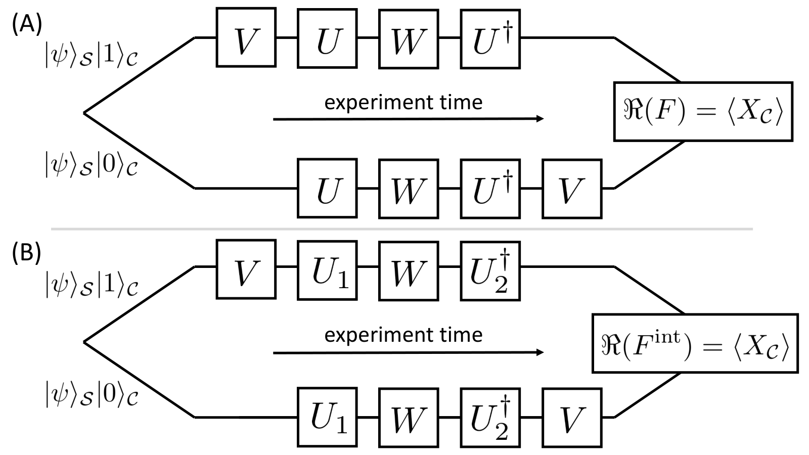
II.2 Imperfect Hamiltonian evolution in the interferometric scheme

The forward and/or reverse evolution might be implemented imperfectly: Some unitary $U_{1}=e^{-iH_{1}t}$ might be implemented instead of $U$ , and $U_{2}^{\dagger}=e^{iH_{2}t}$ might be implemented instead of $U^{\dagger}$ . The Hamiltonians $H_{1}$ and $H_{2}$ may differ slightly from the ideal $H$ . As a result, $H_{2}$ might not equal $-H_{1}$ . The reverse evolution would not “undo” the forward evolution: $U_{2}^{\dagger}U_{1}\neq\mathbbm{1}$ .

Multiple sources can corrupt the evolution, including imperfect control of analog tuning. Consider attempting to negate the Hamiltonian by turning a knob, which determines the angle through which a qubit is rotated, from $\theta$ to $-\theta$ . The knob might be turned slightly past the $-\theta$ point. Zhu et al. mitigate analog errors with a “quantum clock” in [25]. Their Hamiltonian’s sign depends on the state of a control qubit ${\mathcal{C}^{\prime}}$ . If ${\mathcal{C}^{\prime}}$ occupies the state $\lvert 1\rangle$ , ${\mathcal{S}}$ evolves under $U$ . If ${\mathcal{C}^{\prime}}$ occupies $\lvert 0\rangle$ , ${\mathcal{S}}$ evolves under $U^{\dagger}$ . A magnitude- $\pi$ rotation flips ${\mathcal{C}^{\prime}}$ . The renormalization scheme (i) mitigates the error independently and (ii) eliminates error incurred by depolarization of the control qubit ${\mathcal{C}^{\prime}}$ (Sec. IV.2).

Renormalization mitigates also errors that threaten both the analog and quantum-clock protocols. Each spin may experience a small, random external magnetic field. Additionally, the coupling strengths may vary randomly.

II.3 Derivation of renormalization scheme for interferometer measurements

Suppose that ${\mathcal{S}}{\mathcal{C}}$ evolves imperfectly. The joint system ends not in the state $\lvert\Psi^{\prime}\rangle$ [Eq. (2)], but in

\displaystyle\lvert\Psi_{12}^{\prime}\rangle=\frac{1}{\sqrt{2}}(VU_{2}^{\dagger}WU_{1}\lvert\psi\rangle\otimes\lvert 0\rangle+U_{2}^{\dagger}WU_{1}V\lvert\psi\rangle\otimes\lvert 1\rangle)\,.

(3)

By measuring the control’s $\sigma^{x}$ , one can reconstruct

\displaystyle\left\langle X_{\mathcal{C}}\right\rangle=\Re\bm{(}{F_{t}^{\rm int}}(V,W)\bm{)}\,,

(4)

wherein

\displaystyle{F_{t}^{\rm int}}(V,W)

\displaystyle:=\left\langle U_{1}^{\dagger}W^{\dagger}U_{2}V^{\dagger}U_{2}^{\dagger}WU_{1}V\right\rangle

(5)

approximates $F_{t}$ . The superscript “int” signals that ${F_{t}^{\rm int}}(V,W)$ is inferred from the interferometric protocol.

Consider “shielding” each $W$ from its imperfect-unitary neighbors by inserting identities $\mathbbm{1}=UU^{\dagger}$ :

	$\displaystyle{F_{t}^{\rm int}}(V,W)$	$\displaystyle=\langle U_{1}^{\dagger}(UU^{\dagger})W^{\dagger}(UU^{\dagger})U_{2}V^{\dagger}$
		$\displaystyle\qquad\times U_{2}^{\dagger}(UU^{\dagger})W(UU^{\dagger})U_{1}V\rangle\,.$		(6)

Regrouping the unitaries, and recalling that $W_{t}=U^{\dagger}WU$ , yields

	$\displaystyle{F_{t}^{\rm int}}(V,W)$	$\displaystyle=\langle(U_{1}^{\dagger}U)W^{\dagger}_{t}(U^{\dagger}U_{2})V^{\dagger}(U_{2}^{\dagger}U)$
		$\displaystyle\qquad\times W_{t}(U^{\dagger}U_{1})V\rangle\,.$		(7)

Let us define a “perturbed $V$ ” through

\displaystyle{V_{\rm int}}^{\dagger}:=(U^{\dagger}U_{2})V^{\dagger}(U_{2}^{\dagger}U)\,.

(8)

We insert a $V^{\dagger}V$ , formed from unperturbed unitaries, beside the perturbed ${V_{\rm int}}^{\dagger}$ in Eq. (7):

	$\displaystyle{F_{t}^{\rm int}}(V,W)$	$\displaystyle=\langle(U_{1}^{\dagger}U)W^{\dagger}_{t}V^{\dagger}(V{V_{\rm int}}^{\dagger})$
		$\displaystyle\qquad\times W_{t}(U^{\dagger}U_{1})V\rangle\,.$		(9)

Suppose that we could eliminate the $(U_{1}^{\dagger}U)$ , $(V{V_{\rm int}}^{\dagger})$ , and $(U^{\dagger}U_{1})$ . ${F_{t}^{\rm int}}(V,W)$ would reduce to $F_{t}$ . We will “divide out” the undesirable factors, loosely speaking.

Consider setting $W$ to $\mathbbm{1}$ , then repeating the interferometry protocol. This deformed protocol should require less control than the ordinary protocol. One would infer

\displaystyle{F_{t}^{\rm int}}(\mathbbm{1},V)=\left\langle(U_{1}^{\dagger}U){V_{\rm int}}^{\dagger}(U^{\dagger}U_{1})V\right\rangle\,.

(10)

This expectation value is of the undesirable factors, rearranged, in Eq. (9). Hence dividing (9) by (10) is expected to approximate the OTOC:

\displaystyle\boxed{F_{t}\approx\frac{{F_{t}^{\rm int}}(W,V)}{{F_{t}^{\rm int}}(\mathbbm{1},V)}}\,.

(11)

The approximation is expected to be strong when the denominator is sizable: Dividing by a number close to zero would lead to an instability. ${F_{t}^{\rm int}}(W,V)$ remains close to zero starting after the scrambling time, $t_{*}$ (defined as the time at which the OTOC begins to deviate significantly from unity). Hence Eq. (11) is expected to hold until approximately $t=t_{*}$ , and the scrambling time can be inferred from renormalized data.

Equation (11) is a conjecture that we have motivated analytically. Numerical support appears in Sec. II.4; and an analytic calculation for a holographic model, in Sec. V. Appendix A motivates (11) alternatively with an infinite-temperature limit.

Another motivating limit consists of the trivial OTOC. Consider setting $W=V=\mathbbm{1}$ . Every function in Eq. (11) reduces to one. The left-hand side equals the right-hand side in this simple case.

II.4 Numerical simulations of the interferometer

We consider a model of $n$ qubits with power-law decaying Ising interactions in a one-dimensional chain with open boundary conditions—the power-law quantum Ising model. The model’s Hamiltonian is

H_{\rm P}=-\sum_{\ell=1}^{\ell_{0}}\sum_{r=1}^{n-\ell}\frac{J}{\ell^{\zeta}}\sigma^{z}_{r}\sigma^{z}_{r+\ell}-\sum_{r}h^{x}\sigma^{x}_{r}-\sum_{r}h^{z}_{r}\sigma^{z}_{r},

(12)

wherein $J$ sets the interaction-energy scale, $\zeta$ and $\ell_{0}$ control the interaction range, $h^{x}$ denotes the transverse field, and $h^{z}_{r}$ denotes a position-dependent longitudinal field.

Most of the numerical data shown below correspond to $n=14$ , $J=1$ , $\zeta=6$ , $\ell_{0}=5$ , $h^{x}=1.05$ , and $h^{z}_{r}=.375(-1)^{r}$ . The OTOC operators are chosen to be $V=\sigma^{x}_{1}$ and $W=\sigma^{x}_{n}$ . The renormalization scheme’s power does not depend on these parameter choices. But this combination is illustrative, causing OTOCs to grow approximately exponentially at early times. Simple exponential growth has proven rare in many researchers’ numerical studies of small, local spin chains.

One might expect the power-law quantum Ising model to be realizable with immediate- and near-term quantum many-body platforms. Possible examples include the Rydberg-atom ensemble in [35]. A similar Hamiltonian has been considered independently in [36].

The system’s initial state is taken to be either the all- $(+y)$ state or a state drawn randomly from the Hilbert space. The $+y$ state is a simple product state in the energy spectrum’s center. The random state mimics the maximally mixed state’s physics. Mixed states are inconvenient to study with the sparse-matrix techniques employed in these numerics; random pure states serve as proxies. Similar results can be obtained from other initial states, including states away from the energy spectrum’s center.

The imperfect interferometric scheme is defined as follows. Starting from $H_{\rm P}$ , we define the forward Hamiltonian $H_{1}$ and the backward Hamiltonian $H_{2}$ . These are related to $H_{\rm P}$ by the addition of random time-independent perturbations, including nearest-neighbor $\sigma^{z}\sigma^{z}$ couplings and onsite $\sigma^{z}$ and $\sigma^{x}$ fields, all of strength $\varepsilon$ :

	$\displaystyle H_{1}$	$\displaystyle-H_{\rm P}=$
		$\displaystyle\varepsilon\sum_{r=1}^{n-1}\eta^{(1)}_{zz,r}\sigma^{z}_{r}\sigma^{z}_{r+1}+\varepsilon\sum_{r=1}^{n}\eta^{(1)}_{x,r}\sigma^{x}_{r}+\varepsilon\sum_{r=1}^{n}\eta^{(1)}_{z,r}\sigma^{z}_{r}\,,$		(13)

and

	$\displaystyle H_{2}$	$\displaystyle-H_{\rm P}=$
		$\displaystyle\varepsilon\sum_{r=1}^{n-1}\eta^{(2)}_{zz,r}\sigma^{z}_{r}\sigma^{z}_{r+1}+\varepsilon\sum_{r=1}^{n}\eta^{(2)}_{x,r}\sigma^{x}_{r}+\varepsilon\sum_{r=1}^{n}\eta^{(2)}_{z,r}\sigma^{z}_{r}.$		(14)

Each of $\eta^{(i)}_{zz,r}$ , $\eta^{(i)}_{z,r}$ , and $\eta^{(i)}_{x,r}$ is a random variable drawn uniformly from $\left[-\frac{1}{2},\,\frac{1}{2}\right]$ . Each run involves one instance of $H_{1}$ and one instance of $H_{2}$ . Each plot shows the OTOC’s real part, unless otherwise stated. All times are measured in units in which the nearest-neighbor coupling $J=1$ .

Figures 2 and 3 show the results of one run of the renormalization scheme for $n=14$ spins with $\varepsilon=.2$ and the all- $(+y)$ initial state. This choice of $\varepsilon$ corresponds to imperfections that are $\pm 10\%$ of the nearest-neighbor coupling, a quite sizable perturbation. Nevertheless, while the imperfect signal deviates substantially from the ideal result, the renormalized value remains close to the ideal up to scrambling time.

Figures 4 and 5 show the results of one run with $\varepsilon$ reduced to $\varepsilon=.1$ . Now, the agreement between the ideal and the renormalized values is remarkable at early times. Yet the two values still diverge somewhat after the scrambling time. Outside the regime in which the renormalization is expected to approximate $F$ , i.e., after $t_{*}$ , the imperfect value tracks the ideal OTOC better than the renormalized value does. We can also push the results in the opposite direction, considering $\varepsilon=.3$ , as shown in Figures 6 and 7. Clearly, the renormalized value’s quality decreases as $\varepsilon$ increases. But, even here, the early-time agreement is reasonable.

We can also check the system-size dependence. Substantially increasing the system size to $n=18$ , with $\varepsilon=.2$ , leads to Figures 8 and 9. The quality of the early-time match between the ideal and renormalized values is of comparable quality to the $n=14$ quality. But the time scale at which the two deviate is noticeably earlier, though still around the scrambling time.

The renormalized value’s quality depends also on the initial state. For example, if we choose a random initial state, the renormalized value matches the ideal result better. Such a random state mimics a maximally mixed state. Hence the renormalization scheme could work best with the infinite-temperature state. This likelihood is promising for nuclear-magnetic-resonance (NMR) experiments, whose initial states tend to be highly mixed [29, 31]. Numerical results for $n=14$ spins and a random initial state are shown in Figures 10 and 11. As claimed, the agreement between the renormalized and ideal values is enhanced relative to the all- $(+y)$ initial state.

III Example #2: Weak measurement

Weak measurements can be used to infer the OTOC experimentally. A weak measurement barely disturbs the measured system. Refraining from damaging the quantum state is often desirable but comes with a tradeoff: A weak measurement extracts little information. But averaging over weak-measurement trials reproduces strong-measurement statistics. Also, weak measurements offer experimental access to OTOCs and to more-fundamental quasiprobabilities [11, 12].

The weak-measurement protocol for inferring the OTOC is detailed in Appendix A of [11] and is simplified in [12, Sec. II].¹¹ 1 Let $n$ denote the number of degrees of freedom, e.g., the number of spins in a chain. In the original protocol, each measured observable $O$ equals a product of $n$ local operators $O_{j}$ : $O=\otimes_{j=1}^{n}O_{j}$ . In the simplified protocol, each observable nontrivially transforms just one spin. We focus on the simplified protocol, though the renormalization scheme is expected to extend to the original protocol.

Figure 12 reviews the weak-measurement protocol. Hamiltonian errors are modeled, and the renormalization approximation is derived, in Sec. III.1. Numerical simulations in Sec. III.2 support the scheme.

III.1 Derivation of renormalization scheme for weak-measurement data

The weak-measurement circuit contains a forward evolution $U$ , followed by a reverse evolution $U^{\dagger}$ , followed by another $U$ . Each evolution might be implemented imperfectly. We denote the implemented unitaries by $U_{1}:=e^{-iH_{1}t}$ , $U_{2}^{\dagger}:=e^{iH_{2}t}$ , and $U_{3}:=e^{-iH_{3}t}$ . The erroneous Hamiltonians $H_{1},H_{2},H_{3}\neq H$ .

From many imperfect weak-measurement trials, one can infer the approximation

	$\displaystyle{\tilde{\mathscr{A}}_{\rho}^{\rm wk}}(v_{1},w_{2},v_{2},w_{3})$	$\displaystyle:={\rm Tr}(U_{1}^{\dagger}U_{2}U_{3}^{\dagger}\Pi^{W}_{w_{3}}U_{3}\Pi^{V}_{v_{2}}$
		$\displaystyle\qquad\quad\times U_{2}^{\dagger}\Pi^{W}_{w_{2}}U_{1}\Pi^{V}_{v_{1}}\rho)$		(15)

to the OTOC. Equation (15) follows from Eq. (37) of [12]. More generally,

\displaystyle{F_{t}^{\rm wk}}(A,B,C,D):={\rm Tr}\left(U_{1}^{\dagger}U_{2}U_{3}^{\dagger}A^{\dagger}U_{3}B^{\dagger}U_{2}^{\dagger}CU_{1}D\rho\right)\,.

(16)

Consider “shielding” each $W$ from its imperfect-unitary neighbors with factors of $\mathbbm{1}=UU^{\dagger}$ . We regroup unitaries, then recall $W_{t}:=U^{\dagger}WU$ :

	$\displaystyle{F_{t}^{\rm wk}}(W,V,W,V)$	$\displaystyle={\rm Tr}\bm{(}[U_{1}^{\dagger}U_{2}U_{3}^{\dagger}U]W^{\dagger}_{t}[U^{\dagger}U_{3}V^{\dagger}U_{2}^{\dagger}U]$
		$\displaystyle\qquad\quad\times W_{t}[U^{\dagger}U_{1}V]\rho\bm{)}\,.$		(17)

We would almost recover the OTOC if we could replace the $U^{\dagger}U_{3}^{\dagger}V^{\dagger}U_{2}^{\dagger}U$ with $V^{\dagger}$ and the $U^{\dagger}U_{1}V$ with $V$ . Let us ape the replacement. We insert an $\mathbbm{1}=VV^{\dagger}$ rightward of the $U^{\dagger}U_{3}^{\dagger}V^{\dagger}U_{2}^{\dagger}U$ and one leftward of the $U^{\dagger}U_{1}V$ . Regrouping unitaries yields

	$\displaystyle{F_{t}^{\rm wk}}(W,V,W,V)$	$\displaystyle={\rm Tr}\bm{(}[U_{1}^{\dagger}U_{2}U_{3}^{\dagger}U]W^{\dagger}_{t}[U^{\dagger}U_{3}V^{\dagger}U_{2}^{\dagger}UV]$
		$\displaystyle\qquad\times V^{\dagger}W_{t}V[V^{\dagger}U^{\dagger}U_{1}V]\rho\bm{)}\,.$		(18)

Equation (18) would equal the OTOC if the bracketed factors were removed. One might expect the bracketed factors to have roughly the size

		$\displaystyle{\rm Tr}\left([U_{1}^{\dagger}U_{2}U_{3}^{\dagger}U][U^{\dagger}U_{3}V^{\dagger}U_{2}^{\dagger}UV][V^{\dagger}U^{\dagger}U_{1}V]\rho\right)$
		$\displaystyle\qquad={\rm Tr}\left(U_{1}^{\dagger}U_{2}V^{\dagger}U_{2}^{\dagger}U_{1}V\rho\right)$		(19)
		$\displaystyle\qquad={F_{t}^{\rm wk}}(\mathbbm{1},V,\mathbbm{1},V)\,.$		(20)

We wish to remove the bracketed factors’ influence on ${F_{t}^{\rm wk}}(W,V,W,V)$ . One might attempt to do so by dividing (18) by (20):

\displaystyle F_{t}\approx\frac{{F_{t}^{\rm wk}}(W,V,W,V)}{{F_{t}^{\rm wk}}(\mathbbm{1},V,\mathbbm{1},V)}\,.

(21)

But consider setting $V$ to $\mathbbm{1}$ . The left-hand side reduces to one. So does the right-hand side’s denominator. But the numerator evaluates to

		$\displaystyle{\rm Tr}\bm{(}U_{1}^{\dagger}U_{2}U_{3}^{\dagger}W^{\dagger}U_{3}U_{2}^{\dagger}WU_{1}\rho\bm{)}$		(22)
		$\displaystyle={F_{t}^{\rm wk}}(W,\mathbbm{1},W,\mathbbm{1})\,.$		(23)

Hence we divide the right-hand side of Eq. (21) by (22):

\displaystyle\boxed{F_{t}\approx\frac{{F_{t}^{\rm wk}}(W,V,W,V)}{{F_{t}^{\rm wk}}(\mathbbm{1},V,\mathbbm{1},V)\,{F_{t}^{\rm wk}}(W,\mathbbm{1},W,\mathbbm{1})}}\,.

(24)

The weak-measurement conjecture (24) requires a $W$ -dependent factor. The interferometer conjecture (11) does not. Why, physically?

The Hamiltonian is negated only once in the interferometry protocol. Hence equating $V$ with $\mathbbm{1}$ in Eq. (5) enables the $U_{2}$ to cancel the $U_{2}^{\dagger}$ . That cancellation frees the $W^{\dagger}$ to cancel the $W$ . Hence ${F_{t}^{\rm int}}(V,W)$ reduces to one if $V=\mathbbm{1}$ , regardless of what $W$ equals.

In contrast, the Hamiltonian is negated twice in the weak-measurement protocol. $U_{3}$ can fail to equal $U_{2}$ . Hence the $U_{3}$ in Eq. (22) can fail to cancel the $U_{2}^{\dagger}$ , despite $V$ ’s equaling $\mathbbm{1}$ . Hence the $W^{\dagger}$ cannot “reach” the $W$ to cancel it. A $W$ -dependent factor must be divided out in (24).

III.2 Numerical simulations of the weak-measurement scheme

We numerically study the weak-measurement renormalization scheme in Eq. (24). For simplicity, we restrict to chaotic parameters of the power-law quantum Ising model. Various other limits give similar results, however. All the plots below are for a system size of $n=12$ . This choice is merely numerically convenient: Larger sizes requires sparse-matrix techniques, and the weak-measurement scheme requires simulations of three time evolutions. (In contrast, the interferometric scheme requires that only two time evolutions be simulated.)

Figures 13 and 14 compare the ideal, imperfect, and renormalized values of a weak measurement of the OTOC. Each of $U_{1}$ , $U_{2}$ , and $U_{3}$ is generated by a Hamiltonian that differs from the ideal by an amount $\varepsilon=.2$ . (See Eq. (13) and the surrounding discussion.) Even for this large value of $\varepsilon$ , and though the weak-measurement scheme involves three imperfect time evolutions (instead of only two), the early-time agreement between the ideal and renormalized values remains reasonably good.

Figures 15 and 16 show the same situation, except with a random initial state, instead of an all $+y$ initial state. As with the interferometric renormalization scheme, the random state leads to improved agreement at early times and a longer period of agreement at later times.

Figures 17 and 18 show the weak-measurement renormalization scheme with $\varepsilon=.1$ . Downsizing the error improves the agreement between the ideal and renormalized signals. There is some disagreement at very early times. But the signal there is already so small, we expect it to be difficult to access with near-term experiments.

IV Decoherence by the environment

Sections II and III detailed how to infer about $F_{t}$ from protocols marred by Hamiltonian errors. Unitaries modeled the evolutions. But the environment can couple to the system [37, 38, 39]. The state can evolve under a nonunitary channel $\mathcal{E}$ [40]. Nevertheless, we show, renormalization facilitates the recovery of $F_{t}$ .

$F_{t}$ can be recovered perfectly despite two instances of decoherence. First, Garttner et al. have measured an OTOC of over 100 trapped ions [30]. We generalize their measurement scheme in Sec. IV.1. We then suppose that the ions’ state depolarizes probabilistically. Renormalization enables the retrieval of $F_{t}$ , an analytical proof shows, without channel tomography.

Second, we return to the interferometric measurement of Sec. II. We suppose that the control qubit suffers probabilistic decoherence. Again, renormalization enables the inference of $F_{t}$ without channel tomography.

Section IV.3 complements the analytics with numerics. The power-law quantum Ising model is coupled to another spin chain. The interaction and environmental Hamiltonians remain unchanged as the system Hamiltonian is reversed.

IV.1 Exact recovery of $F_{t}$ despite probabilistic depolarization of the system during a generalization of the ion-trap protocol

The ion-trap experiment in [30] motivates this section. We review their protocol in Sec. IV.1.1 and generalize their set-up in Sec. IV.1.2. The system could decohere during each unitary evolution. We model decoherence with probabilistic depolarization. Section IV.1.3 concerns the ideal limit. Section IV.1.4 concerns the general case. The exact value of $F_{t}$ can be extracted via renormalization. The extraction requires no channel tomography.

IV.1.1 Motivation: Ion-trap protocol

Garttner et al. implemented the following protocol:

1.

Prepare the ions in the eigenstate $\lvert\mathord{\hbox to8.4pt{\vbox to8.4pt{\pgfpicture\makeatletter\hbox{\hskip 0.5pt\lower-0.5pt\hbox to0.0pt{\lxSVG@begingroup@{_scopebegin=1} \lxSVG@begingroup@{stroke=#000000} \lxSVG@begingroup@{fill=#000000} \lxSVG@setlinewidth{\the\pgflinewidth}\lxSVG@begingroup@{stroke-width=0.4pt} \lx@inpgf@ignorespaces\nullfont\hbox to0.0pt{\lxSVG@begingroup@{_scopebegin=1} {{\lx@inpgf@ignorespaces}}\lxSVG@setlinewidth{\the\pgflinewidth}\lxSVG@begingroup@{stroke-width=1.0pt} \lx@inpgf@ignorespaces {}{{}}{} {}{}{}\lxSVG@stroke\lxSVG@drawpath@unclipped{M 5.12 0 L 5.12 10.24}{fill:none} \lx@inpgf@ignorespaces {}{{}}{} {}{}{}\lxSVG@stroke\lxSVG@drawpath@unclipped{M 0 5.12 L 10.24 5.12}{fill:none} \lx@inpgf@ignorespaces \lxSVG@closescope {\lx@inpgf@ignorespaces}{\lx@inpgf@ignorespaces}{\lx@inpgf@ignorespaces}\hss}\lxSVG@discardpath\lxSVG@closescope \hss}}\lxSVG@closescope\endpgfpicture}}}\rangle:=\lvert+\rangle^{\otimes n}$ of the Pauli product $\otimes_{j=1}^{n}\sigma_{j}^{x}$ .
2.

Evolve the system forward in time under the all-to-all Ising Hamiltonian $H=\frac{J}{n}\sum_{i<j}\sigma^{z}_{i}\sigma^{z}_{j}$ . The coupling strength is denoted by $J$ .
3.

Rotate the qubits counterclockwise through an angle $\phi$ about the $x$ -axis, with²² 2 This $W$ acts nontrivially on every qubit. A conventional $W$ , described in earlier sections, acts nontrivially on just a small subsystem. Experimental practicalities motivated the many-qubit $W$ . But this $W$ equals a product of single-qubit operators. See [30] for further discussion. $W=e^{-i\phi\sum_{j}\sigma^{x}_{j}}$ .
4.

Evolve the system backward, under $-H$ .

Measure the $i^{\rm th}$ spin’s $x$ -component, $V=\sigma^{x}_{i}$ , for any $i=1,2,\ldots,n$ . The value of $i$ does not matter, due to the system’s translational invariance. Averaging the outcomes over trials yields the expectation value

		$\displaystyle\langle\mathord{\hbox to8.4pt{\vbox to8.4pt{\pgfpicture\makeatletter\hbox{\hskip 0.5pt\lower-0.5pt\hbox to0.0pt{\lxSVG@begingroup@{_scopebegin=1} \lxSVG@begingroup@{stroke=#000000} \lxSVG@begingroup@{fill=#000000} \lxSVG@setlinewidth{\the\pgflinewidth}\lxSVG@begingroup@{stroke-width=0.4pt} \lx@inpgf@ignorespaces\nullfont\hbox to0.0pt{\lxSVG@begingroup@{_scopebegin=1} {{\lx@inpgf@ignorespaces}}\lxSVG@setlinewidth{\the\pgflinewidth}\lxSVG@begingroup@{stroke-width=1.0pt} \lx@inpgf@ignorespaces {}{{}}{} {}{}{}\lxSVG@stroke\lxSVG@drawpath@unclipped{M 5.12 0 L 5.12 10.24}{fill:none} \lx@inpgf@ignorespaces {}{{}}{} {}{}{}\lxSVG@stroke\lxSVG@drawpath@unclipped{M 0 5.12 L 10.24 5.12}{fill:none} \lx@inpgf@ignorespaces \lxSVG@closescope {\lx@inpgf@ignorespaces}{\lx@inpgf@ignorespaces}{\lx@inpgf@ignorespaces}\hss}\lxSVG@discardpath\lxSVG@closescope \hss}}\lxSVG@closescope\endpgfpicture}}}\|U^{\dagger}e^{i\phi\sum_{j}\sigma^{x}_{j}}U\sigma^{x}_{i}U^{\dagger}e^{-i\phi\sum_{j}\sigma^{x}_{j}}U\sigma^{x}_{i}\|\mathord{\hbox to8.4pt{\vbox to8.4pt{\pgfpicture\makeatletter\hbox{\hskip 0.5pt\lower-0.5pt\hbox to0.0pt{\lxSVG@begingroup@{_scopebegin=1} \lxSVG@begingroup@{stroke=#000000} \lxSVG@begingroup@{fill=#000000} \lxSVG@setlinewidth{\the\pgflinewidth}\lxSVG@begingroup@{stroke-width=0.4pt} \lx@inpgf@ignorespaces\nullfont\hbox to0.0pt{\lxSVG@begingroup@{_scopebegin=1} {{\lx@inpgf@ignorespaces}}\lxSVG@setlinewidth{\the\pgflinewidth}\lxSVG@begingroup@{stroke-width=1.0pt} \lx@inpgf@ignorespaces {}{{}}{} {}{}{}\lxSVG@stroke\lxSVG@drawpath@unclipped{M 5.12 0 L 5.12 10.24}{fill:none} \lx@inpgf@ignorespaces {}{{}}{} {}{}{}\lxSVG@stroke\lxSVG@drawpath@unclipped{M 0 5.12 L 10.24 5.12}{fill:none} \lx@inpgf@ignorespaces \lxSVG@closescope {\lx@inpgf@ignorespaces}{\lx@inpgf@ignorespaces}{\lx@inpgf@ignorespaces}\hss}\lxSVG@discardpath\lxSVG@closescope \hss}}\lxSVG@closescope\endpgfpicture}}}\rangle$
		$\displaystyle=\langle\mathord{\hbox to8.4pt{\vbox to8.4pt{\pgfpicture\makeatletter\hbox{\hskip 0.5pt\lower-0.5pt\hbox to0.0pt{\lxSVG@begingroup@{_scopebegin=1} \lxSVG@begingroup@{stroke=#000000} \lxSVG@begingroup@{fill=#000000} \lxSVG@setlinewidth{\the\pgflinewidth}\lxSVG@begingroup@{stroke-width=0.4pt} \lx@inpgf@ignorespaces\nullfont\hbox to0.0pt{\lxSVG@begingroup@{_scopebegin=1} {{\lx@inpgf@ignorespaces}}\lxSVG@setlinewidth{\the\pgflinewidth}\lxSVG@begingroup@{stroke-width=1.0pt} \lx@inpgf@ignorespaces {}{{}}{} {}{}{}\lxSVG@stroke\lxSVG@drawpath@unclipped{M 5.12 0 L 5.12 10.24}{fill:none} \lx@inpgf@ignorespaces {}{{}}{} {}{}{}\lxSVG@stroke\lxSVG@drawpath@unclipped{M 0 5.12 L 10.24 5.12}{fill:none} \lx@inpgf@ignorespaces \lxSVG@closescope {\lx@inpgf@ignorespaces}{\lx@inpgf@ignorespaces}{\lx@inpgf@ignorespaces}\hss}\lxSVG@discardpath\lxSVG@closescope \hss}}\lxSVG@closescope\endpgfpicture}}}\|W^{\dagger}_{t}V^{\dagger}W_{t}V\|\mathord{\hbox to8.4pt{\vbox to8.4pt{\pgfpicture\makeatletter\hbox{\hskip 0.5pt\lower-0.5pt\hbox to0.0pt{\lxSVG@begingroup@{_scopebegin=1} \lxSVG@begingroup@{stroke=#000000} \lxSVG@begingroup@{fill=#000000} \lxSVG@setlinewidth{\the\pgflinewidth}\lxSVG@begingroup@{stroke-width=0.4pt} \lx@inpgf@ignorespaces\nullfont\hbox to0.0pt{\lxSVG@begingroup@{_scopebegin=1} {{\lx@inpgf@ignorespaces}}\lxSVG@setlinewidth{\the\pgflinewidth}\lxSVG@begingroup@{stroke-width=1.0pt} \lx@inpgf@ignorespaces {}{{}}{} {}{}{}\lxSVG@stroke\lxSVG@drawpath@unclipped{M 5.12 0 L 5.12 10.24}{fill:none} \lx@inpgf@ignorespaces {}{{}}{} {}{}{}\lxSVG@stroke\lxSVG@drawpath@unclipped{M 0 5.12 L 10.24 5.12}{fill:none} \lx@inpgf@ignorespaces \lxSVG@closescope {\lx@inpgf@ignorespaces}{\lx@inpgf@ignorespaces}{\lx@inpgf@ignorespaces}\hss}\lxSVG@discardpath\lxSVG@closescope \hss}}\lxSVG@closescope\endpgfpicture}}}\rangle\,.$		(25)

The ions could couple to the environment during either evolution. A quantum channel $\mathcal{E}$ would evolve the system’s state [40]. We model the channel with probabilistic depolarization. The environment has some probability of mapping the state to the maximally mixed state $\mathbbm{1}/d$ , wherein $d$ denotes the Hilbert space’s dimensionality.

IV.1.2 General set-up

Let ${\mathcal{S}}$ denote a quantum system associated with a Hilbert space $\mathcal{H}$ of dimensionality ${\rm dim}(\mathcal{H})=d$ . In [30], ${\mathcal{S}}$ consists of $n$ qubits. Hence $d=2^{n}$ .

The natural Hamiltonian $H$ generates the ideal evolution $U:=e^{-iHt}$ . The actual evolution is imperfect: ${\mathcal{S}}$ has a probability $p\in[0,1]$ of undergoing $U$ and a probability $1-p$ of depolarizing totally to $\mathbbm{1}/d$ . This probabilistic depolarization evolves a state $\sigma$ as

\displaystyle{\mathcal{E}_{p}^{\rm depol}}(\sigma)=p\,U\sigma U^{\dagger}+(1-p)\frac{\mathbbm{1}}{d}\,.

(26)

The reverse evolution is ideally $U^{\dagger}$ . The actual evolution has a probability $1-q$ of depolarizing the state completely:

\displaystyle{\tilde{\mathcal{E}}_{q}^{\rm depol}}(\sigma)=q\,U^{\dagger}\sigma U+(1-q)\frac{\mathbbm{1}}{d}\,.

(27)

The forward and reverse probabilities need not equal each other: $p\neq q$ . An experimentalist need not know the probabilities’ values, to infer $F_{t}$ : Renormalization will cancel $p$ and $q$ from the calculation.

The operators $W$ and $V$ are unitary: $W^{\dagger}W=V^{\dagger}V=\mathbbm{1}$ . Additionally, $V$ is Hermitian and traceless: $V^{\dagger}=V$ , and ${\rm Tr}(V)=0$ . Pauli operators satisfy these assumptions.

Let $v$ denote an arbitrary eigenvalue of $V$ . Let $\lambda_{v}$ denote the set of degeneracy parameters for the $v$ eigenspace. ${\mathcal{S}}$ begins in a state $\rho$ supported just in the $v$ eigenspace:

\displaystyle\rho=\sum_{\lambda_{v},\lambda_{v}^{\prime}}q_{\lambda_{v},\lambda_{v}^{\prime}}\lvert v,\lambda_{v}\rangle\!\langle v,\lambda_{v}^{\prime}\rvert\,.

(28)

The coefficients satisfy the normalization condition $|q_{\lambda_{v},\lambda_{v}^{\prime}}|^{2}=1$ .

The protocol proceeds as follows: ${\mathcal{S}}$ is prepared in the state $\rho$ . The system is evolved under ${\mathcal{E}_{p}^{\rm depol}}$ , then under $W$ , then under ${\tilde{\mathcal{E}}_{q}^{\rm depol}}$ . The system ends in the state

	$\displaystyle\rho^{\prime}$	$\displaystyle:={\tilde{\mathcal{E}}_{q}^{\rm depol}}\bm{(}W{\mathcal{E}_{p}^{\rm depol}}(\rho)W^{\dagger}\bm{)}$		(29)
		$\displaystyle=pq\,W_{t}\rho W_{t}^{\dagger}+(1-pq)\frac{\mathbbm{1}}{d}\,.$		(30)

$V$ is measured. This process is repeated in each of many trials. Averaging the outcomes yields the expectation value ${\rm Tr}(V\rho^{\prime})$ . The renormalization scheme requires also a set of trials in which $W=\mathbbm{1}$ .

IV.1.3 Ideal case

Suppose that $p=q=1$ . The system ends in the state $\rho^{\prime}_{\rm ideal}=W_{t}\rho W^{\dagger}_{t}$ . The expectation value of $V$ becomes

\displaystyle{\rm Tr}(V\rho^{\prime}_{\rm ideal})={\rm Tr}(VW_{t}\rho W^{\dagger}_{t})={\rm Tr}\bm{(}W^{\dagger}_{t}V^{\dagger}W_{t}\rho\bm{)}\,.

(31)

The second equality follows from the trace’s cyclicality and the Hermiticity of $V$ . By Eq. (28), $\frac{V}{v}\rho=\rho$ . Hence inserting a $V/v$ leftward of $\rho$ yields

\displaystyle\frac{1}{v}{\rm Tr}(V\rho^{\prime}_{\rm ideal})=F_{t}\,.

(32)

The expectation value is proportional to the OTOC.

IV.1.4 Imperfect evolution and renormalization

The expectation value of $V$ becomes

	$\displaystyle{F_{{t},{p},{q}}^{\rm depol}}(W,V)$	$\displaystyle:={\rm Tr}(V\rho^{\prime})$		(33)
		$\displaystyle=\frac{pq}{v}F_{t}\,.$		(34)

This expression follows from the tracelessness of $V$ .

$W$ must equal $\mathbbm{1}$ in another set of trials. The expectation value of $V$ reduces to

\displaystyle{F_{{t},{p},{v}}^{\rm depol}}(\mathbbm{1},V)=pqv\,,

(35)

by $V\rho=v\rho$ and the normalization of $\rho$ .

Consider dividing the right-hand side of Eq. (34) by the right-hand side of Eq. (35). The quotient is proportional to the OTOC:

\displaystyle\boxed{F_{t}=v^{2}\>\frac{{F_{{t},{p},{q}}^{\rm depol}}(W,V)}{{F_{{t},{p},{q}}^{\rm depol}}(\mathbbm{1},V)}}\,.

(36)

IV.2 Exact recovery of $F_{t}$ despite probabilistic depolarization of the control qubit in the interferometric protocol

The interferometric protocol relies on a control qubit ${\mathcal{C}}$ (Sec. II.1). ${\mathcal{C}}$ is prepared in the state $\lvert+\rangle$ . Suppose that it decoheres. We model the decoherence with probabilistic depolarization:

	$\displaystyle\lvert+\rangle\!\langle+\rvert$	$\displaystyle\mapsto p\lvert+\rangle\!\langle+\rvert+(1-p)\,\frac{\mathbbm{1}}{2}$		(37)
		$\displaystyle=\frac{1}{2}[\lvert 0\rangle\!\langle 0\rvert+\lvert 1\rangle\!\langle 1\rvert+p(\lvert 0\rangle\!\langle 1\rvert+\lvert 1\rangle\!\langle 0\rvert)]\,.$		(38)

The joint system-and-control state $\lvert\Psi\rangle$ must be replaced with

\displaystyle\rho_{{\mathcal{S}}{\mathcal{C}}}

\displaystyle=\lvert\psi\rangle\!\langle\psi\rvert\otimes\frac{1}{2}[\lvert 0\rangle\!\langle 0\rvert+\lvert 1\rangle\!\langle 1\rvert+p(\lvert 0\rangle\!\langle 1\rvert+\lvert 1\rangle\!\langle 0\rvert)]\,.

(39)

The interferometer maps the joint state to

$\displaystyle\rho^{\prime}_{{\mathcal{S}}{\mathcal{C}}}$	$\displaystyle=\frac{1}{2}[VW_{t}\lvert\psi\rangle\!\langle\psi\rvert W_{t}V\otimes\lvert 0\rangle\!\langle 0\rvert+W_{t}V\lvert\psi\rangle\!\langle\psi\rvert VW_{t}\otimes\lvert 1\rangle\!\langle 1\rvert$
	$\displaystyle\qquad+p(VW_{t}\lvert\psi\rangle\!\langle\psi\rvert VW_{t}\otimes\lvert 0\rangle\!\langle 1\rvert$
	$\displaystyle\qquad\qquad+W_{t}V\lvert\psi\rangle\!\langle\psi\rvert W_{t}V\otimes\lvert 1\rangle\!\langle 0\rvert)]\,.$	(40)

We recast $\rho^{\prime}_{{\mathcal{S}}{\mathcal{C}}}$ in terms of the eigenstates $\lvert+\rangle$ and $\lvert-\rangle$ of the control’s $\sigma^{x}$ :

$\displaystyle\rho^{\prime}_{{\mathcal{S}}{\mathcal{C}}}$	$\displaystyle=\frac{1}{4}[(VW_{t}\lvert\psi\rangle\!\langle\psi\rvert W_{t}V+W_{t}V\lvert\psi\rangle\!\langle\psi\rvert VW_{t}$
	$\displaystyle\qquad+pVW_{t}\lvert\psi\rangle\!\langle\psi\rvert VW_{t}+pW_{t}V\lvert\psi\rangle\!\langle\psi\rvert W_{t}V)\otimes\lvert+\rangle\!\langle+\rvert$
	$\displaystyle\quad+(VW_{t}\lvert\psi\rangle\!\langle\psi\rvert W_{t}V+W_{t}V\lvert\psi\rangle\!\langle\psi\rvert VW_{t}$
	$\displaystyle\qquad-pVW_{t}\lvert\psi\rangle\!\langle\psi\rvert VW_{t}-pW_{t}V\lvert\psi\rangle\!\langle\psi\rvert W_{t}V)\otimes\lvert-\rangle\!\langle-\rvert$
	$\displaystyle\qquad\;+(\text{cross-terms})]\,.$	(41)

The control’s $\sigma^{x}$ has the expectation value

\displaystyle\left\langle X\right\rangle_{\mathcal{C}}^{(W,V,p)}=p\,\Re(F_{t})\,.

(42)

The expectation value is proportional to the signal. The “not depolarized” probability $p$ reduces the signal.

Consider repeating the protocol with $V=W=\mathbbm{1}$ . The expectation value becomes

\displaystyle\left\langle X\right\rangle_{\mathcal{C}}^{(\mathbbm{1},\mathbbm{1},p)}=p\,.

(43)

Renormalizing the right-hand side of Eq. (42) with the right-hand side of Eq. (43) yields the OTOC’s real part:

\displaystyle\boxed{\Re(F_{t})=\frac{\left\langle X\right\rangle_{\mathcal{C}}^{(W,V,p)}}{\left\langle X\right\rangle_{\mathcal{C}}^{(\mathbbm{1},\mathbbm{1},p)}}}\,.

(44)

The OTOC can be inferred perfectly, without approximation. Furthermore, the not-depolarized probability $p$ can be inferred in the absence of channel tomography, which costs substantial time and classical computation.

IV.3 Numerical simulations of decoherence

To explore the physics of environmental decoherence numerically, we adopt the following simple model. We consider two equal-length chains of the power-law quantum Ising model, a system chain $\cal{S}$ and an environment chain $\cal{E}$ . The Hamiltonian is

\displaystyle H_{\cal{S}\cal{E}}=H_{\cal{S}}+H_{\cal{E}}+J_{\rm c}\sum_{i=1}^{n_{\cal{S}}}\sigma^{z}_{i}\sigma^{z}_{i+n_{\cal{S}}}\,,

(45)

wherein $H_{\cal{S}}$ and $H_{\cal{E}}$ are power-law-quantum-Ising Hamiltonians, the system consists of qubits $\{1,...,n_{\cal{S}}\}$ , and the environment consists of qubits $\{n_{\cal{S}}+1,...,2n_{\cal{S}}\}$ . Each system qubit $i$ couples to the corresponding environmental qubit $i$ .

In the time-reversal procedure, the forward Hamiltonian is

\displaystyle H_{1}=H_{\cal{S}\cal{E}}=H_{\cal{S}}+H_{\cal{E}}+J_{\rm c}\sum_{i=1}^{n_{\cal{S}}}\sigma^{z}_{i}\sigma^{z}_{i+n_{\cal{S}}}\,,

(46)

and the backward Hamiltonian is

\displaystyle H_{2}=H_{\cal{S}\cal{E}}=H_{\cal{S}}-H_{\cal{E}}-J_{\rm c}\sum_{i=1}^{n_{\cal{S}}}\sigma^{z}_{i}\sigma^{z}_{i+n_{\cal{S}}}\,.

(47)

Only the system Hamiltonian is reversed.

Figures 19 and 20 show the results of our interferometric renormalization scheme applied to this situation when $J_{\rm c}=.2$ . There is now significant deviation at early times on the semilogarithmic plot. But, given how crude this time-reversal procedure is and how strong the coupling is, the agreement remains reasonably good. The early-time growth rate, as extracted from the renormalized data, is still much closer to the ideal result than the imperfect data is.

Figures 21 and 22 show the same scheme, with a reduced $J_{\rm c}=.1$ . Now, not only is the imperfect data relatively close to the ideal result, but the renormalized data also cleaves very closely to the ideal result even well after the scrambling time for the small sizes considered here. So, while these models differ substantially from the simple depolarization channel in Sec. IV.1, we find a similar conclusion about the renormalization scheme’s efficacy in mitigating environmental decoherence.

V Holographic model

Let us show that the conclusions above are not accidents of small system size, of the models considered, or of infinite temperature. We perform an analytical calculation in a strongly chaotic system, using the holographic anti-de-Sitter-space/conformal-field-theory (AdS/CFT) duality. The renormalization formula holds for simple timing errors, even at finite temperatures, up to the scrambling time. The timing error is the simplest imperfection that can studied holographically: The forward and backward time evolutions last for different lengths of time. In the language above, $H_{1}$ are $H_{2}$ proportional, but not generally equal, to $H$ .

As stated, the goal is to show that the renormalization formula works in a highly nontrivial setting far beyond the system sizes explored in the numerical simulations. However, the calculation should not be viewed as a useless toy model: Engineering a controlled quantum many-body system that would exhibit a version of holographic duality is a realistic experimental goal (e.g., [30, 41, 35, 42]). Such a system would allow experimental access to black-hole scrambling. Hence it is sensible to assess the robustness of scrambling measurements in highly chaotic systems dual to gravity.

Let the forward-evolution time be $t_{1}=t+\delta_{1}$ , and let the reverse time be $t_{2}=t+\delta_{2}$ . If $\rho$ is a thermal state $e^{-\beta H}/Z$ , the imperfect OTOC is

\tilde{F}_{t}=\text{Tr}(W^{\dagger}_{t}V^{\dagger}_{-\delta_{2}}W_{t}V_{-\delta_{1}}\rho),

(48)

wherein, again, $O_{t}:=e^{iHt}Oe^{-iHt}$ is a Heisenberg-picture operator.

Two simplifications prove convenient in the holographic calculation: First, $V$ is assumed to be Hermitian. Second, we deform the OTOC to a thermally regulated OTOC. Thermal regulation does not change the essential physics of scrambling in this model. We consider a thermally regulated version of $\tilde{F}_{t}$ of the form

\tilde{F}_{t}^{\text{reg}}=\text{Tr}(W^{\dagger}_{t}V_{-\delta_{2}}W_{t}\sqrt{\rho}V_{-\delta_{1}}\sqrt{\rho})\,.

(49)

Other thermal regulations are possible. This choice is convenient because it captures the physics of scrambling and maps cleanly to a geometric problem.³³ 3 Consider a general thermal correlation function $\langle A(t_{1})B(t_{2})C(t_{3})D(t_{4})\rangle$ . What we call “thermal regulation” amounts to shifting some of the time arguments by imaginary terms. The imaginary-time evolution operator is proportional to a power of $e^{-\beta H}/Z$ . This analytic continuation therefore amounts to breaking $\rho$ into pieces and distributing them amongst $A$ , $B$ , $C$ , and $D$ . See, for example, [7].

$\tilde{F}_{t}^{\text{reg}}$ is related to the expectation value of the tensor product of $V$ with its transpose, $V_{-\delta_{2}}\otimes\left(V_{-\delta_{1}}\right)^{T}$ , in a doubled system. By “doubled system,” we mean two copies of the system of interest. The relevant whole-system state results from having perturbed the thermofield double with $W$ . The thermofield double

|\text{TFD}\rangle=\sum_{i}\sqrt{\frac{e^{-\beta E_{i}}}{Z}}|E_{i}\rangle\otimes|E_{i}\rangle

(50)

purifies the thermal $\rho$ . The perturbed thermofield double state is

|W\rangle=\left(W_{t}\otimes\mathbbm{1}\right)|\text{TFD}\rangle\,.

(51)

Hence

\tilde{F}_{t}^{\text{reg}}=\langle W|V_{-\delta_{2}}\otimes\left(V_{-\delta_{1}}\right)^{T}|W\rangle.

(52)

We define the transpose using the energy basis, such that $\left(O_{t}\right)^{T}=\left(O^{T}\right)_{-t}$ and

\tilde{F}_{t}^{\text{reg}}=\langle W|V_{-\delta_{2}}\otimes\left(V^{T}\right)_{\delta_{1}}|W\rangle.

(53)

This expectation value is related, via the AdS/CFT duality, to a correlation function between the two sides of an eternal black hole perturbed by a shock wave caused by $W$ .

Assume that the shock wave does not add much energy to the system. The bulk geometry is described by a mass- $M$ black hole perturbed, on the horizon, by a shock wave with a null shift $\alpha$ . $M$ is determined by the thermal-state temperature $1/\beta$ (we set Boltzmann’s constant to $k_{\mathrm{B}}=1$ ). The details of this geometry are recorded in [5]. Let $t=-t_{w}$ denote the long-ago time at which $W$ perturbed the system.⁴⁴ 4 $t$ is often assumed to be positive. But the same physics results for negative $t$ in the thermal state, if $W$ and $V$ are exchanged. Since this model’s scrambling physics does not depend strongly on $W$ and $V$ , we are free to choose the most convenient sign for $t$ . Let $\delta E$ denote the energy added to the system by $W$ . In a convenient Kruskal coordinate system, the perturbation shifts the coordinates in the left-hand geometry relative the right-hand coordinates by an amount $\alpha=\frac{\delta E}{4M}e^{2\pi t_{w}/\beta}$ .

$\tilde{F}_{t}^{\text{reg}}$ will be analyzed in a geodesic approximation. Consider the two boundary points at which the $V$ operators are inserted. The renormalized geodesic distance between these points is

\frac{d}{\ell}\bigg|_{\text{ren}}=2\log\left(\cosh\left(\frac{\pi(t_{\rm L}-t_{\rm R})}{\beta}\right)+\frac{\alpha}{2}e^{-\pi(t_{\rm L}+t_{\rm R})/\beta}\right),

(54)

wherein $\ell$ denotes the AdS radius, Planck’s constant $\hbar=1$ , and $t_{\rm L}$ and $t_{\rm R}$ denote the times at which the $V$ ’s operate on the left and right boundaries. In our case, $t_{\rm L}=\delta_{2}$ , and $t_{\rm R}=\delta_{1}$ . “Renormalized” refers, here, to the removal of field-theory divergences, not to the renormalization formula (11). In fact, the field-theory renormalizations cancel from the renormalization formula’s numerator and denominator.

Let $V$ be a primary field with dimension $\Delta$ (and bulk mass $\sim\Delta/\ell$ ). The geodesic approximation to the correlator is

\tilde{F}_{t}^{\text{reg}}\sim\left(\frac{1}{\cosh\left(\frac{\pi(\delta_{2}-\delta_{1})}{\beta}\right)+\frac{\alpha}{2}e^{-\pi(\delta_{2}+\delta_{1})/\beta}}\right)^{2\Delta}.

(55)

Let us expand in small $\alpha$ , as is reasonable until just before the scrambling time, $t_{*}$ :

	$\displaystyle\tilde{F}_{t}^{\text{reg}}\sim$	$\displaystyle\left(\frac{1}{\cosh\left(\frac{\pi(\delta_{2}-\delta_{1})}{\beta}\right)}\right)^{2\Delta}$			(56)
		$\displaystyle\times\left(1-\Delta\alpha\frac{e^{-\pi(\delta_{1}+\delta_{2})/\beta}}{\cosh\left(\frac{\pi(\delta_{2}-\delta_{1})}{\beta}\right)}+\cdots\right).$			(56)

Typically, many experimental shots are required to build up enough statistics to estimate the value of $F_{t}$ . This process will be complicated if the values of $\delta_{1}$ and $\delta_{2}$ vary from shot to shot. The sensible thing to do is to (i) average over shots, to estimate the values of $\tilde{F}_{t}(W,V)$ and $\tilde{F}_{t}(\mathbbm{1},V)$ separately, and then (ii) take the ratio to estimate $F_{t}$ via the renormalization formula. Would such a procedure yield nearly the correct value of $F_{t}$ ?

V.1 Simple error distribution

Let $\delta_{i}=\pm\epsilon t_{w}$ with probability $1/2$ for $i=1,2$ : In every shot, the system has a probability $1/2$ of being over-evolved for a fraction $\epsilon$ of the total time and a probability $1/2$ of being under-evolved analogously. To reduce notation, we relabel the renormalization-formula numerator as $A_{1}=\tilde{F}_{t}^{\text{reg}}(W,V)$ and the denominator as $A_{2}=\tilde{F}_{t}^{\text{reg}}(\mathbbm{1},V)$ . The shot-average of $A_{2}$ is

\overline{A_{2}}=\frac{1}{2}+\frac{1}{2}\frac{1}{\left[\cosh\left(\frac{2\pi\epsilon t_{w}}{\beta}\right)\right]^{2\Delta}}.

(57)

Similarly, the shot-average of $A_{1}$ , to leading order in $\alpha$ , is

\displaystyle\overline{A_{1}}=\overline{A_{2}}-\frac{\Delta\alpha}{2}\left[\frac{1}{\left[\cosh\left(\frac{2\pi\epsilon t_{w}}{\beta}\right)\right]^{2\Delta+1}}+\cosh\left(\frac{2\pi\epsilon t_{w}}{\beta}\right)\right].

(58)

We can check the limit as $\epsilon t_{w}\rightarrow 0$ : $\overline{A_{2}}\rightarrow 1$ , and $\overline{A_{1}}\rightarrow 1-\Delta\alpha$ , which are the ideal values. The renormalized value for general $\epsilon t_{w}$ but small $\alpha$ is

1-\Delta\alpha\frac{\left[\cosh\left(\frac{2\pi\epsilon t_{w}}{\beta}\right)\right]^{2\Delta+2}+1}{\left[\cosh\left(\frac{2\pi\epsilon t_{w}}{\beta}\right)\right]^{2\Delta+1}+\cosh\left(\frac{2\pi\epsilon t_{w}}{\beta}\right)}\,.

(59)

Suppose that the timing error is severe: $\epsilon t_{w}\gg\beta$ . The measured correlators limit as $\overline{A_{2}}\rightarrow 1/2$ and $\overline{A_{1}}\rightarrow 1/2-\Delta\alpha e^{2\pi\epsilon t_{w}/\beta}/4+\ldots$ The renormalization formula becomes

\frac{\>\;\overline{A_{1}}\;\>}{\overline{A_{2}}}\to 1-\Delta\alpha\frac{e^{2\pi\epsilon t_{w}/\beta}}{2}+\ldots

(60)

Recall that (i) the ideal value is $F=1-\Delta\alpha+\cdots$ and (ii) $\alpha=\frac{\delta E}{4M}e^{2\pi t_{w}/\beta}$ . Substituing shot-averaged quantities into the renormalization formula therefore gives exponential growth. The exponent differs from the ideal value by no more than a factor of $\epsilon$ .

We can also study the renormalization scheme away from small $\alpha$ . The general results are

\overline{A_{2}}=\frac{1}{2}+\frac{1}{2}\frac{1}{\left[\cosh\left(\frac{2\pi\epsilon t_{w}}{\beta}\right)\right]^{2\Delta}}

(61)

and

	$\displaystyle\overline{A_{1}}=$	$\displaystyle\frac{1}{4}\left(\frac{1}{1+\frac{\alpha}{2}e^{-2\pi\epsilon t_{w}/\beta}}\right)^{2\Delta}+\frac{1}{4}\left(\frac{1}{1+\frac{\alpha}{2}e^{+2\pi\epsilon t_{w}/\beta}}\right)^{2\Delta}$
		$\displaystyle+\frac{1}{2}\left(\frac{1}{\cosh\left(\frac{2\pi\epsilon t_{w}}{\beta}\right)+\frac{\alpha}{2}}\right)^{2\Delta}.$		(62)

These results are illustrated Figures 23 and 24. The scheme’s quality is excellent even for a 10 $\%$ timing error ( $\epsilon=0.1$ ). More precisely, the correct exponential growth is encoded in $\alpha\sim e^{2\pi t/\beta}$ . The renormalization formula predicts an exponential growth of $e^{2\pi(1+\epsilon)t/\beta}$ . Hence even in this strongly chaotic model of many degrees of freedom⁵⁵ 5 Let us reparameterize the null shift as $\alpha\equiv Ge^{2\pi t/\beta}$ , wherein $G:=\frac{\delta E}{4M}$ . The entropy $S$ scales as $1/G$ , wherein $G$ plays the role of Newton’s constant. (Assume that the energy perturbation obeys $\delta E\sim 1/\beta$ . Since $M\sim S/\beta$ , $\frac{\delta E}{M}\sim\frac{1}{S}$ . Hence $G\sim\frac{\delta E}{M}\sim\frac{1}{S}$ . Similarly, the entropy $S_{\rm BH}$ of a general black hole varies inversely with Newton’s constant: $S_{\rm BH}\propto\frac{1}{G_{\rm N}}$ ; hence our use of the notation $G$ .) at finite temperature, the renormalization scheme estimates the correct exponent to relative error of order $\epsilon$ .

VI Conclusions

We have shown, with analytical arguments and numerical simulations, that scrambling measurements are remarkably resilient with respect to imperfections in the experimental protocol. Our physical interpretation of the results is that the physics of scrambling can be cleanly separated from the decay of fidelity due to imperfections, up to the scrambling time. We exhibited this resilience for a chaotic local spin chain of up to $n=18$ sites and for a strongly chaotic holographic model with many degrees of freedom. We have checked that our conclusions apply also many other models. Examples include integrable models and nonlocal models (e.g., the Sachdev-Ye-Kitaev (SYK) model [43, 6, 44, 45]). We focused on states near the energy spectrum’s center. But the renormalization scheme applies to other states, e.g., the ground state. Thus, the resilience of scrambling measurements shown here is quite general.

In the numerical analysis, we considered mostly modest system sizes. The choice facilitates the study of many models and set-ups with a reasonable amount of computer time. We studied a few larger system sizes, however—up to $n=20$ spins. We found, at most, a modest degradation in the renormalization scheme’s effectiveness until the scrambling time. Precisely how the renormalization scheme’s effectiveness scales with $n$ remains an open question. The holographic analysis, which applies to a system with many degrees of freedom, gives evidence of a favorable scaling with system size. Experiments should be able to create headway.

Perhaps our results’ most important consequences are for experiments. Our renormalization schemes are simple and general and should greatly enhance early experiments’ abilities to probe the physics of scrambling. For example, imperfections in the time-reversal scheme appear readily addressable with our methods. To that end, it would be very interesting to study in detail our renormalization scheme, with realistic assumptions, in the context of various near term experimental platforms.

Along these lines, one unrealistic assumption made in the numerical analysis was that the imperfections were the identical in all experimental runs. We lift this assumption in Appendix B: The renormalization formula, phrased in terms of shot-averaged quantities, remains valid despite shot-to-shot variations in the imperfections.

Our results also enable the use of new approximate time-reversal schemes. For example, consider reversing only the fields and the odd-index-neighbor couplings in the power-law quantum Ising model. This scheme may seem artificial. But consider an experiment in which local fields are easy to control but the interactions are fixed. Local unitary transformations and field reversal can effect such a partial time reversal. Such a reversal, combined with our renormalization scheme, gives excellent agreement with the ideal-time-reversal results.

Testing the scheme in larger experimental systems would help illuminate our renormalization scheme’s physics. Indeed, the quantum physics of near-term noisy quantum devices presents an exciting frontier today [46]. Our results suggest that scrambling might be amenable to study on noisy near-term machines. Relatedly, a similar procedure of dividing by a Loschmidt echo has been used in analysis of nuclear-magnetic-resonance experiments [47].

In our quest to better understand our resilience results’ significance, calculations in model systems will be valuable. The numerics here form a black-box approach. More insight may come from opening the box, budding off from the holographic calculation in Sec. V and the decoherence models in Sec. IV. Perhaps the physics of scrambling resilience can be related to known types of robustness, e.g., the robustness of renormalization-group fixed points. It would be interesting to probe resilience in many other recently studied models, including noninteracting, weakly coupled, and semiclassical systems [48, 49, 50, 15, 51, 52], many-body-localized states [53, 54, 55, 56, 57], the SYK model [43, 6, 44, 45], open systems [37], local random-circuit models [58, 59, 60, 61], other special solvable models [28], and much else.

Finally, an extension of the renormalization scheme to the out-of-time-ordered-correlator (OTOC) quasiprobability $\tilde{\mathscr{A}}_{\rho}$ merits further study. Two approaches suggest themselves: (i) The analytical argument of Sec. III.1 might be modified: Projectors $\Pi^{W}_{w_{\ell}}$ and $\Pi^{V}_{v_{\ell}}$ might replace the unitaries $W$ and $V$ . Yet $\Pi^{V}_{v_{\ell}}$ lacks the unitary property $V^{\dagger}V=\mathbbm{1}$ . Perhaps this lack can be circumvented. (ii) Suppose that the eigenvalues of $W$ and the eigenvalues of $V$ equal $\pm 1$ . (Suppose, for example, that $W$ and $V$ are Paulis.) $\tilde{\mathscr{A}}_{\rho}$ equals a combination of $F_{t}$ and simpler correlators [12, Sec. II D]. $F_{t}$ can be renormalized, we have shown. Each simpler correlator needs no renormalization, or appears to be renormalizable generally, or appears to be renormalizable under certain conditions on $\rho$ (e.g., if $\rho=\mathbbm{1}/d$ ). Renormalizing every term, then assembling the terms, is expected to yield a renormalized OTOC quasiprobability.

Acknowledgements.

NYH is grateful for funding from the Institute for Quantum Information and Matter, an NSF Physics Frontiers Center (NSF Grant PHY-1125565) with support of the Gordon and Betty Moore Foundation (GBMF-2644); for partial support from the Walter Burke Institute for Theoretical Physics at Caltech; for a Graduate Fellowship from the Kavli Institute for Theoretical Physics; for a Barbara Groce Graduate Fellowship; and to Justin Dressel for weak-measurement discussions. BGS is supported by the Simons Foundation, through the “It From Qubit Collaboration,” and by the National Science Foundation, under Grant No. NSF PHY-1125915, and acknowledges useful discussions with Monika Schleier-Smith and Norm Yao.

Appendix A Further motivation for renormalization of the interferometer: Infinite-temperature analysis

Consider inputting an infinite-temperature state, $\rho=\mathbbm{1}/2^{n}$ , into the imperfect interferometer:

\displaystyle F^{\text{int}}_{t}=\frac{1}{2^{n}}\text{Tr}\left(U_{1}^{\dagger}W^{\dagger}U_{2}V^{\dagger}U_{2}^{\dagger}WU_{1}V\right).

(A1)

Define $V_{i}:=U^{\dagger}U_{i}VU_{i}^{\dagger}U$ , such that

\displaystyle F^{\text{int}}_{t}=\frac{1}{2^{n}}\text{Tr}\left(W^{\dagger}_{t}V_{2}^{\dagger}W_{t}V_{1}\right).

(A2)

Consider inserting an identity operator $\mathbbm{1}=V^{\dagger}V$ leftward of the $V_{2}^{\dagger}$ :

\displaystyle F^{\text{int}}_{t}=\frac{1}{2^{n}}\text{Tr}\left(W^{\dagger}_{t}V^{\dagger}\left[VV_{2}^{\dagger}\right]W_{t}V_{1}\right).

(A3)

Since $\left(VV_{2}^{\dagger}\right)W_{t}=W_{t}\left(VV_{2}^{\dagger}\right)+\left[VV_{2}^{\dagger},W_{t}\right]$ ,

	$\displaystyle F^{\text{int}}_{t}$	$\displaystyle=\frac{1}{2^{n}}\text{Tr}\left(W^{\dagger}_{t}V^{\dagger}W_{t}V\left[V_{2}^{\dagger}V_{1}\right]\right)$
		$\displaystyle\quad+\frac{1}{2^{n}}\text{Tr}\left(W^{\dagger}_{t}V^{\dagger}\left[VV_{2}^{\dagger},W_{t}\right]V_{1}\right).$		(A4)

We can motivate the renormalization scheme by approximating the first term as

		$\displaystyle\frac{1}{2^{n}}\text{Tr}\left(W^{\dagger}_{t}V^{\dagger}W_{t}V\left[V_{2}^{\dagger}V_{1}\right]\right)$
		$\displaystyle\approx\frac{1}{2^{n}}\text{Tr}\left(W^{\dagger}_{t}V^{\dagger}W_{t}V\right)\frac{1}{2^{n}}\text{Tr}\left(V_{2}^{\dagger}V_{1}\right),$		(A5)

and approximating the second term as

\displaystyle\frac{1}{2^{n}}\text{Tr}\left(W^{\dagger}_{t}V^{\dagger}\left[VV_{2}^{\dagger},W_{t}\right]V_{1}\right)\approx 0.

(A6)

The first approximation is motivated by the fact that it becomes exact as $W\rightarrow\mathbbm{1}$ or if $[W_{t},V]\approx 0$ . Hence the approximation is expected to be good until roughly the scrambling time.

The second approximation is motivated by the fact that matrix elements of commutators—objects of the form $\frac{1}{2^{n}}\text{Tr}(A[B,C])$ —are generically small in chaotic, and in perturbed integrable, systems. More precisely, consider early times at which, by Trotter-expanding in the perturbation strength $\varepsilon$ , one can approximate $V_{i}\approx V+O(\varepsilon)$ . The second term should be smaller than the signal by at least a factor of $\varepsilon$ .

At later times, approximating $V_{i}\approx V$ is no longer possible. By typical matrix elements of commutators are expected to be small due to chaos—inherent or arising from perturbed integrability. One can object that $\frac{1}{2^{n}}\text{Tr}(W_{t}^{\dagger}V^{\dagger}[W_{t},V])$ and $\frac{1}{2^{n}}\text{Tr}(V^{\dagger}W_{t}^{\dagger}[W_{t},V])$ approach $\mp 1$ , respectively, at late times in a chaotic system. These examples appear to violate expectations. This anomaly arises, however, because the operators inside and outside the commutator are finely attuned to each other. This tuning is absent from the second term above.

Even away from infinite temperature, aspects of the above discussion can be imitated. Consider feeding the perturbed interferometer a general pure state $|\psi\rangle$ :

\displaystyle F^{\text{int}}_{t}=\langle\psi|U_{1}^{\dagger}W^{\dagger}U_{2}V^{\dagger}U_{2}^{\dagger}WU_{1}V|\psi\rangle.

(A7)

Let $|\tilde{\psi}\rangle:=U^{\dagger}U_{1}|\psi\rangle$ , such that

\displaystyle F^{\text{int}}_{t}=\langle\tilde{\psi}|W_{t}^{\dagger}V_{2}^{\dagger}W_{t}V_{1}|\tilde{\psi}\rangle.

(A8)

Repeating the infinite-temperature analysis suggests that

\displaystyle F^{\text{int}}_{t}\approx\langle\tilde{\psi}|W_{t}^{\dagger}V^{\dagger}W_{t}V|\tilde{\psi}\rangle\langle\tilde{\psi}|V_{2}^{\dagger}V_{1}|\tilde{\psi}\rangle.

The second term is

\displaystyle\langle\tilde{\psi}|V_{2}^{\dagger}V_{1}|\tilde{\psi}\rangle=F^{\text{int}}_{t}(\mathbbm{1},V),

(A9)

the denominator in the renormalization scheme.

The first term has an appealing OTOC form, but $\lvert\tilde{\psi}\rangle$ has replaced $\lvert\psi\rangle$ . How are the states’ OTOCs related? In a chaotic system, any thermalized state’s energy density is expected to determine the state’s scrambling physics in the thermodynamic limit. Hence we must ask (i) is $|\tilde{\psi}\rangle$ a thermalized state and (ii) how does the energy density of $|\tilde{\psi}\rangle$ differ from that of $|\psi\rangle$ ?

By late times—as the commutator-squared $|[W(t),V]|^{2}$ grows appreciably—we expect $|\tilde{\psi}\rangle$ to be thermalized with respect to Hamiltonian $H$ . After all, the state has evolved under $H$ for a long (negative) time.

Furthermore, we expect the state’s average energy to be $\langle\tilde{\psi}|H|\tilde{\psi}\rangle\approx\langle\psi|H_{1}|\psi\rangle$ . To see why, think of $|\tilde{\psi}\rangle$ as arising from two evolutions. $U_{1}$ governs the first evolution; and $U^{\dagger}$ , the second. As $U^{\dagger}$ evolves the system, the expectation value of $H$ is conserved:

\displaystyle\langle\tilde{\psi}|H|\tilde{\psi}\rangle=\langle\psi|U_{1}^{\dagger}HU_{1}|\psi\rangle.

(A10)

The Hamiltonian decomposes as $H=H_{1}+(H-H_{1})$ . The $U_{1}$ evolution generically conserves only the first term. (Other conserved quantities can affect the analysis, but we neglect this complication.) Suppose that the $H_{1}$ evolution is chaotic. (Even when $H$ is integrable, we expect the typical perturbation not to be.) The expectation value of $H-H_{1}$ will decay with time. Hence

\displaystyle\langle\tilde{\psi}|H|\tilde{\psi}\rangle\approx\langle\psi|H_{1}|\psi\rangle.

(A11)

In the thermodynamic limit, the energy density should control the scrambling dynamics, e.g., by setting the effective system temperature. Suppose that $H_{1}$ differs from $H$ by a systematic deviation of order $\varepsilon$ . The energy density of $|\tilde{\psi}\rangle$ should differ from the energy density of $|\psi\rangle$ by an amount of order $\varepsilon$ . This result constitutes the worst case. Suppose now that, as in the numerical examples studied above, $H_{1}$ differs from $H$ by a random local deviation. The total difference in energy is expected to be proportional to $\sqrt{n}$ , instead of to $n$ . The difference in energy density is of order $\varepsilon/\sqrt{n}$ , which vanishes in the thermodynamic limit.

This analysis suggests that, even away from infinite temperature, the renormalization scheme reproduces the scrambling physics of a state whose energy density differs from that of $|\psi\rangle$ by no more than $\varepsilon$ . Furthermore, if $H_{1}-H$ and $H_{2}-H$ are sums of random terms, the effective energy density is not expected to differ from the actual in the thermodynamic limit. In this case, the renormalization scheme could reproduce the correct energy density’s ideal scrambling dynamics.

These arguments provide some theoretical motivation for the renormalization scheme. But the renormalized numerics’ quality, up to the scrambling time, suggests to us that more remains to be discovered about why the scheme works.

Appendix B Shot-to-shot imperfections

This appendix shows that the renormalization formula also works when the experimental imperfections vary between different experimental shots. This was also the situation considered in the holographic calculation. To minimize computational resources, the numerical results presented are for a Floquet version of the power-law quantum Ising model. Figures 25 and 26 show the interferometric renormalization scheme for a power-law-quantum-Ising Floquet model. Consider one length- $t$ time evolution. The Hamiltonian’s $\sigma^{z}$ terms are pulsed on for a short time $dt$ ; then the $\sigma^{x}$ terms are pulsed on for a time $dt$ ; then the $\sigma^{z}$ terms are pulsed on again; and so on for $t/dt$ time steps. The imperfect time reversal scheme is the Floquet analog of the scheme for the Hamiltonian power-law quantum Ising model (see (13) and surrounding discussion). When $\varepsilon=.2$ , the ideal and renormalized values are quite close.

On the same figures, we show a shot-to-shot version of the renormalization scheme.⁶⁶ 6 Applying the Floquet model to the shot-to-shot study proves convenient: Calculating the Floquet model’s OTOC requires much less computational time that calculating a continuous-time model’s OTOC. This computational advantage enables us to average over many realizations without using too much computer time. In practice, an experimenter performs many runs, or shots, to gather statistics from which to extract the OTOC. What if the perturbations to the Hamiltonians vary from shot to shot? The experimenter can run the experiment many times, infer a shot-averaged imperfect OTOC, and infer a shot-averaged imperfect OTOC whose $W=\mathbbm{1}$ . The experimenter can divide the former shot-averaged OTOC by the latter. That this imperfect ratio equals the ideal is unclear. But the results are surprisingly favorable.

The renormalization formula (11) predicts that, for each shot,

\displaystyle{F_{t}^{\rm int}}(W,V)\approx{F_{t}^{\rm int}}(\mathbbm{1},V)F_{t}.

(B1)

An experimenter typically cannot measure, in one shot, all the quantities in this equation. But $F_{t}$ is the same for every shot. Therefore, the shot-averaged quantities (denoted by overlines) obey

\displaystyle\overline{{F_{t}^{\rm int}}(W,V)}\approx\overline{{F_{t}^{\rm int}}(\mathbbm{1},V)}F_{t}.

(B2)

The difficulty has been removed: The renormalization formula is recast in terms of shot-averaged quantities, which can be measured experimentally.

Averaging over many shots may be advisable generally. The number of shots needed depends on (i) the value of $\varepsilon$ and (ii) how precisely we want to extract the early behavior. Figures 25 and 26 show averages over just 100 samples. The ideal and shot-averaged curves agree reasonably well nonetheless.

References

[1] P. Hayden and J. Preskill, Journal of High Energy Physics 2007, 120 (2007).
[2] Y. Sekino and L. Susskind, Journal of High Energy Physics 2008, 065 (2008).
[3] W. Brown and O. Fawzi, ArXiv e-prints (2012), 1210.6644.
[4] A. Larkin and Y. N. Ovchinnikov, Soviet Journal of Experimental and Theoretical Physics 28 (1969).
[5] S. H. Shenker and D. Stanford, Journal of High Energy Physics 3, 67 (2014).
[6] A. Kitaev, A simple model of quantum holography, KITP strings seminar and Entanglement 2015 program, 2015.
[7] J. Maldacena, S. H. Shenker, and D. Stanford, ArXiv e-prints (2015), 1503.01409.
[8] T. Dray and G. ’t Hooft, Nuclear Physics B 253, 173 (1985).
[9] S. H. Shenker and D. Stanford, Journal of High Energy Physics 5, 132 (2015).
[10] D. A. Roberts and B. Swingle, Phys. Rev. Lett. 117, 091602 (2016).
[11] N. Yunger Halpern, Phys. Rev. A 95, 012120 (2017).
[12] N. Yunger Halpern, B. Swingle, and J. Dressel, ArXiv e-prints (2017), 1704.01971.
[13] M. Campisi and J. Goold, Phys. Rev. E 95, 062127 (2017).
[14] N. Tsuji, T. Shitara, and M. Ueda, Phys. Rev. E 97, 012101 (2018).
[15] I. L. Aleiner, L. Faoro, and L. B. Ioffe, Annals of Physics 375, 378 (2016).
[16] F. M. Haehl, R. Loganayagam, and M. Rangamani, Journal of High Energy Physics 2017, 69 (2017).
[17] F. M. Haehl, R. Loganayagam, and M. Rangamani, Journal of High Energy Physics 2017, 70 (2017).
[18] F. M. Haehl, R. Loganayagam, P. Narayan, and M. Rangamani, ArXiv e-prints (2017), 1701.02820.
[19] P. Hosur, X.-L. Qi, D. A. Roberts, and B. Yoshida, Journal of High Energy Physics 2, 4 (2016), 1511.04021.
[20] D. A. Roberts and B. Yoshida, Journal of High Energy Physics 2017, 121 (2017).
[21] J. Cotler, N. Hunter-Jones, J. Liu, and B. Yoshida, Journal of High Energy Physics 2017, 48 (2017).
[22] N. Hunter-Jones and J. Liu, ArXiv e-prints (2017), 1710.08184.
[23] B. Swingle, G. Bentsen, M. Schleier-Smith, and P. Hayden, Phys. Rev. A 94, 040302 (2016).
[24] N. Y. Yao et al., ArXiv e-prints (2016), 1607.01801.
[25] G. Zhu, M. Hafezi, and T. Grover, ArXiv e-prints (2016), 1607.00079.
[26] I. Danshita, M. Hanada, and M. Tezuka, ArXiv e-prints (2016), 1606.02454.
[27] A. Bohrdt, C. B. Mendl, M. Endres, and M. Knap, New Journal of Physics 19, 063001 (2017).
[28] N. Tsuji, P. Werner, and M. Ueda, Phys. Rev. A 95, 011601 (2017).
[29] J. Li et al., Phys. Rev. X 7, 031011 (2017).
[30] M. Gärttner et al., Nature Physics 13, 781 (2017), Article.
[31] K. X. Wei, C. Ramanathan, and P. Cappellaro, ArXiv e-prints (2016), 1612.05249.
[32] E. J. Meier, J. Ang’ong’a, F. A. An, and B. Gadway, ArXiv e-prints (2017), 1705.06714.
[33] T. Prosen, T. H. Seligman, and M. Žnidarič, Progress of Theoretical Physics Supplement 150, 200 (2003), quant-ph/0304104.
[34] A. Goussev, R. A. Jalabert, H. M. Pastawski, and D. Wisniacki, ArXiv e-prints (2012), 1206.6348.
[35] H. Bernien et al., Nature 551, 579 EP (2017), Article.
[36] X. Chen, T. Zhou, and C. Xu, ArXiv e-prints (2017), 1712.06054.
[37] S. V. Syzranov, A. V. Gorshkov, and V. Galitski, ArXiv e-prints (2017), 1704.08442.
[38] J. R. Gonzalez Alonso, N. Yunger Halpern, and J. Dressel, in prep.
[39] Y.-L. Zhang, Y. Huang, and X. Chen, in prep.
[40] M. A. Nielsen and I. L. Chuang, Quantum Computation and Quantum Information (Cambridge University Press, 2010).
[41] B. Swingle and N. Y. Yao, Physics Viewpoint 10, 82 (2017).
[42] A. Chen, R. Ilan, F. de Juan, D. I. Pikulin, and M. Franz, ArXiv e-prints (2018), 1802.00802.
[43] S. Sachdev and J. Ye, Phys. Rev. Lett. 70, 3339 (1993).
[44] J. Polchinski and V. Rosenhaus, Journal of High Energy Physics 4, 1 (2016), 1601.06768.
[45] J. Maldacena and D. Stanford, ArXiv e-prints (2016), 1604.07818.
[46] J. Preskill, ArXiv e-prints (2018), 1801.00862.
[47] C. M. Sánchez, P. R. Levstein, L. Buljubasich, H. M. Pastawski, and A. K. Chattah, Philosophical Transactions of the Royal Society of London A: Mathematical, Physical and Engineering Sciences 374 (2016).
[48] D. Stanford, Journal of High Energy Physics 10, 9 (2016), 1512.07687.
[49] A. A. Patel and S. Sachdev, ArXiv e-prints (2016), 1611.00003.
[50] A. A. Patel, D. Chowdhury, S. Sachdev, and B. Swingle, ArXiv e-prints (2017), 1703.07353.
[51] D. Chowdhury and B. Swingle, ArXiv e-prints (2017), 1703.02545.
[52] C.-J. Lin and O. I. Motrunich, ArXiv e-prints (2018), 1801.01636.
[53] Y. Huang, Y.-L. Zhang, and X. Chen, ArXiv e-prints (2016), 1608.01091.
[54] R. Fan, P. Zhang, H. Shen, and H. Zhai, ArXiv e-prints (2016), 1608.01914.
[55] R.-Q. He and Z.-Y. Lu, ArXiv e-prints (2016), 1608.03586.
[56] Y. Chen, ArXiv e-prints (2016), 1608.02765.
[57] B. Swingle and D. Chowdhury, ArXiv e-prints (2016), 1608.03280.
[58] A. Nahum, S. Vijay, and J. Haah, (2017), 1705.08975.
[59] C. von Keyserlingk, T. Rakovszky, F. Pollmann, and S. Sondhi, (2017), 1705.08910.
[60] V. Khemani, A. Vishwanath, and D. A. Huse, (2017), 1710.09835.
[61] T. Rakovszky, F. Pollmann, and C. W. von Keyserlingk, (2017), 1710.09827.