跳到论文正文
W Papers独立论文阅读器 arXiv:1802.01367 论文正文 计算阅读时间 · 0%
引用这篇论文根据当前论文元数据生成,正式投稿前建议核对。


License: arXiv.org perpetual non-exclusive license
arXiv:1802.01367v2 [hep-th] 04 Jun 2018

Integrable Subsectors from Holography

Robert de Mello Kocha,b,11 1 robert@neo.phys.wits.ac.za, Minkyoo Kimb,22 2 minkyoo.kim@wits.ac.za

and Hendrik J.R. Van Zylb,33 3 hjrvanzyl@gmail.com

a School of Physics and Telecommunication Engineering,

South China Normal University, Guangzhou 510006, China

b National Institute for Theoretical Physics,

School of Physics and Mandelstam Institute for Theoretical Physics,

University of the Witwatersrand, Wits, 2050,

South Africa

ABSTRACT

We consider operators in 𝒩=4{\cal N}=4 super Yang-Mills theory dual to closed string states propagating on a class of LLM geometries. The LLM geometries we consider are specified by a boundary condition that is a set of black rings on the LLM plane. When projected to the LLM plane, the closed strings are polygons with all corners lying on the outer edge of a single ring. The large NN limit of correlators of these operators receives contributions from non-planar diagrams even for the leading large NN dynamics. Our interest in these fluctuations is because a previous weak coupling analysis argues that the net effect of summing the huge set of non-planar diagrams, is a simple rescaling of the ’t Hooft coupling. We carry out some nontrivial checks of this proposal. Using the s​u​(2|2)2su(2|2)^{2} symmetry we determine the two magnon SS-matrix and demonstrate that it agrees, up to two loops, with a weak coupling computation performed in the CFT. We also compute the first finite size corrections to both the magnon and the dyonic magnon by constructing solutions to the Nambu-Goto action that carry finite angular momentum. These finite size computations constitute a strong coupling confirmation of the proposal.

1 Introduction

There has been dramatic progress in our understanding of 𝒩=4\mathcal{N}=4 super Yang-Mills theory, motivated primarily by the AdS/CFT correspondence [1, 2, 3]. In particular, the dynamics of the subspace of the CFT Hilbert space, spanned by operators with bare dimension JJ with J2N≪1{J^{2}\over N}\ll 1 is integrable in the large NN limit[4, 5]. The discovery of this integrability has enabled an exact computation of the spectrum of anomalous dimensions of the CFT[6]. Being exact, these results are correct even in the strong coupling limit of the theory.

Given this remarkable progress, one would like to know if there are other sectors of the theory, whose dynamics is also integrable. In the article [7] a new integrable sector was proposed and weak coupling evidence for the proposal was given. The subsector consists of small deformations about an LLM geometry[8]. The geometry is labeled by a boundary condition that corresponds to a set of black rings on the LLM plane. The fluctuations propagating on this geometry are closed strings, which when projected to the LLM plane, are polygons with all corners lying on the outer edge of a single ring. The operators corresponding to an LLM background with a closed string excitation have a bare dimension of order N2N^{2}. Consequently we describe these operators using the adjective “heavy”. The large NN limit of the correlators of these heavy operators are not correctly captured by summing only planar diagrams: non-planar diagrams must be included to capture the large NN dynamics. The weak coupling analysis of [7] shows that the net effect of summing this huge class of diagrams is a simple rescaling of the ’t Hooft coupling. This is an interesting result, since it immediately predicts the anomalous dimensions of these operators in terms of the corresponding dimensions computed in the planar limit. It also implies that the dynamics of this subsector is integrable11 1 For independent discussions of the possibility of integrability at the non-planar level see [9, 10].. Our main motivation in this article is to provide some nontrivial checks of the proposal of [7].

The proposal was checked in [7] by computing the one loop anomalous dimensions and then using the s​u​(2|2)2su(2|2)^{2} symmetry[11, 12] to propose an exact dimension. The results agree with the strong coupling prediction obtained from string theory[7]. Further, the s​u​(2|2)2su(2|2)^{2} symmetry can be used to determine the two magnon SS-matrix[11, 12] and this too can be tested in perturbation theory. We will test this SS-matrix against a weak coupling computation performed in the CFT, up to two loops. Our comparison always tests ratios of scattering amplitudes so that we never need the overall pase of the SS-matrix. We find complete agreement between the weak coupling CFT results and the expansion of the exact two magnon SS-matrix.

The skeptical reader will not be convinced: indeed, all quantities compared so far are completely determined by the s​u​(2|2)2su(2|2)^{2} symmetry, so one might wonder how strict these tests are. It is well known that the s​u​(2|2)2su(2|2)^{2} symmetry does not determine the overall phase of the SS-matrix. In this article we test this phase. Specifically, we compute the first finite size corrections to both the magnon and the dyonic magnon. These corrections when computed following Lüscher (see for example [13]) are sensitive to the overall phase of the SS-matrix. We will follow [14] and construct solutions to the Nambu-Goto action that carry finite angular momentum. We are then able to compute the finite size correction at strong coupling. Remarkably these corrections are given by simply rescaling the ’t Hooft coupling (after proper translation to the string theory description) in the AdS5×{}_{5}\timesS5 result. This is a non-trivial strong coupling test that the proposal of [7] passes.

In the next section we will review the construction of the CFT operators belonging to our subsector. We also describe the action of the dilatation operator. Section 3 explains the determination and some weak coupling tests of the two magnon SS-matrix. In section 4 we compute finite size corrections for magnons and dyonic magnons. Our conclusions are presented in section 5.

2 CFT Analysis

The usual lore of the large NN expansion simply does not apply when we consider operators with a bare dimension that scales as N2N^{2}[15, 16, 8, 17]: the pertubation expansion is not organized by the genus of ribbon graphs being summed and the large NN limit is not captured by summing planar diagrams. Fortunately, at least in the free theory, representation theory can be used to provide a basis for the local operators of the theory and to compute the sum of the complete set of ribbon graphs[18, 19, 20, 21, 22, 23, 24, 25]. We will focus on the restricted Schur polynomial basis. As we will see, these operators provide a very natural description of closed strings propagating on an LLM geometry. When loop corrections are considered, operators in the representation theory basis mix only weakly[26, 27, 28, 29, 30, 31, 32, 33, 34]. This is useful since our goal is to diagonalize the dilatation operator.

2.1 Operators dual to LLM geometries

The LLM geometries are regular 12\frac{1}{2}-BPS geometries that are asymptotically A​d​S5×S5AdS_{5}\times S^{5}. These geometries enjoy an R×S​O​(4)×S​O​(4)R\times SO(4)\times SO(4) symmetry [8]. The general LLM geometry is described by the metric (i,j=1,2)(i,j=1,2)

d​s2=−h−2​(d​t+Vi​d​xi)2+h2​(d​y2+d​xi​d​xi)+y​eG​d​Ω3+y​e−G​d​Ω~3,\displaystyle ds^{2}=-h^{-2}(dt+V_{i}dx^{i})^{2}+h^{2}(dy^{2}+dx^{i}dx^{i})+ye^{G}d\Omega_{3}+ye^{-G}d\tilde{\Omega}_{3}, (2.1)

where

h−2=2​y​cosh⁡(G),z=12​tanh⁡(G)y​∂yVi=ϵi​j​∂jz,y⁡(∂iVj−∂jVi)=ϵi​j​∂yz.\displaystyle\begin{array}[]{cc}h^{-2}=2y\cosh(G),&z=\frac{1}{2}\tanh(G)\\ y\partial_{y}V_{i}=\epsilon_{ij}\partial_{j}z,&y(\partial_{i}V_{j}-\partial_{j}V_{i})=\epsilon_{ij}\partial_{y}z.\end{array}

The metric is completely determined by a single function zz which depends on the three coordinates y,x1y,x^{1} and x2x^{2}. It is obtained by solving Laplace’s equation

∂i∂iz+y​∂y∂yzy=0.\displaystyle\partial_{i}\partial_{i}z+y\partial_{y}\frac{\partial_{y}z}{y}=0. (2.5)

To obtain a regular geometry, the boundary conditions for zz on the plane y=0y=0 (which we will refer to as the LLM plane) must be chosen carefully. Regularity requires that z=±12z=\pm\frac{1}{2} on the LLM plane. Any given boundary condition can be represented graphically by coloring the LLM plane black when (z=−12)(z=-\frac{1}{2}) and white when (z=12)(z=\frac{1}{2}) [8].

We will focus on geometries given by concentric black annuli on the LLM plane. Each possible supergravity geometry is dual to a Schur polynomial in the CFT[17]. The Schur polynomial χR​(Z)\chi_{R}(Z) is constructed using a single complex adjoint scalar ZZ. Consequently the ℛ{\cal R} charge JJ and dimension Δ\Delta of this operator are related as Δ=J\Delta=J which is the BPS condition. There is a concrete, explicit map between the Young diagram RR labeling the Schur polynomials and the coloring of the LLM plane. Each Schur polynomial corresponds to a coloring of concentric annuli. Vertical edges in RR correspond to black annuli and horizontal edges to white annuli. The area of each black ring is proportional to the number of rows in the corresponding a vertical edge, while the area of each white ring is proportional to the number of columns in the corresponding horizontal edge. An example of the map between LLM plane colorings and Young diagrams is illustrated in Fig. 1 below.

Refer to caption
Figure 1: An example of the map between Young diagrams and LLM boundary conditions.

For a set of rings having a total of EE edges with radii RlR_{l} l=1,2,…,El=1,2,...,E the geometry is determined by the functions

z=∑l=1E(−1)E−l2​(r2+y2−Rl2(r2+y2+Rl2)2−4​r2​Rl2),z=\sum_{l=1}^{E}{(-1)^{E-l}\over 2}\left({r^{2}+y^{2}-R_{l}^{2}\over\sqrt{(r^{2}+y^{2}+R_{l}^{2})^{2}-4r^{2}R_{l}^{2}}}\right),
Vϕ​(x1,x2,y)=∑l=1E(−1)E−l+12​(r2+y2+Rl2(r2+y2+Rl2)2−4​r2​Rl2−1).V_{\phi}(x^{1},x^{2},y)=\sum_{l=1}^{E}{(-1)^{E-l+1}\over 2}\left({r^{2}+y^{2}+R_{l}^{2}\over\sqrt{(r^{2}+y^{2}+R_{l}^{2})^{2}-4r^{2}R_{l}^{2}}}-1\right).

Finally, given the concrete map between the Young diagram and the LLM boundary condition, when we want to talk about an excitation localized on the LLM plane at the edge of a given annulus we will simply talk about an excitation localized at a corner of the Young diagram.

2.2 Closed strings propagating on LLM geometries

In [7] operators representing excitations localised at a single corner of a Young diagram were constructed. These operators are dual to LLM geometries excited by strings localized at the outer edge of the corresponding annulus. In this section we briefly review the construction of [7] and then extend it to the description of closed string states with a worldsheet that visits the edges of multiple rings. The conjecture we want to test concerns strings localized at a single edge, but we discuss the general case for completeness.

The restricted Schur polynomials are a basis for the local operators of the theory. Consequently, an arbitrary operator OO can be written as a linear combination of restricted Schur polynomials as follows

O=∑R,{r},αaR,{r},α​χR,{r},α​(Z,Y,X,⋯)\displaystyle O=\sum_{R,\{r\},\alpha}a_{R,\{r\},\alpha}\chi_{R,\{r\},\alpha}(Z,Y,X,\cdots) (2.6)

The operator dual to a closed string state is a single trace operator. Focus on a single trace operator OO, given by the trace of a product of fields of the 𝒩=4{\cal N}=4 super Yang-Mills theory. These fields may be adjoint scalars, adjoint fermions or covariant derivatives of these fields[35, 36]. If we use a total of kk species of fields then {r}\{r\} is a collection of kk Young diagrams, one for each species. If we use nin_{i} fields of species ii the corresponding Young diagram rir_{i} has nin_{i} boxes. The Young diagram r1r_{1} corresponds to the ZZ field. The Young diagram RR has n1+n2+…+nkn_{1}+n_{2}+...+n_{k} boxes. The additional labels contained in α\alpha are discrete labels distinguishing operators that carry the same R,{r}R,\{r\} labels.

We will, as usual, think of the single trace operator as a one dimensional lattice. All fields which are not ZZs are impurities and we record their position on the lattice. Thus, the operator O⁡({l1=1,l2=4})O(\{l_{1}=1,l_{2}=4\}) corresponds to a trace Tr⁡(Y​Z2​Y​ZJ−2){\rm Tr\,}(YZ^{2}YZ^{J-2}).

Suppose now that we consider a closed string excitation of an LLM geometry, attached to a particular corner of the Young diagram BB describing the LLM geometry. The proposal of [7] is that this operator is simply given by

OB=∑R,{r},αaR,{r},α​χRB,{r1​B,r2,⋯,rk},α​(Z)\displaystyle O_{B}=\sum_{R,\{r\},\alpha}a_{R,\{r\},\alpha}\chi_{R_{B},\{r_{1B},r_{2},\cdots,r_{k}\},\alpha}(Z) (2.7)

The coefficients appearing in the sum (2.7) are identical to the coefficients appearing in (2.6). Including the background implies that we have included an enormous number of extra ZZ fields. Consequently, the Young diagrams RR and r1r_{1}, both of which are sensitive to the number of ZZ fields, are modified as indicated above. RBR_{B} (or rBr_{B}) is obtained by attaching RR (or rr) to the relevant corner of the background Young diagram BB.

The operator OBO_{B} is significantly more complicated than the single trace operator OO. Indeed, it has a complicated multitrace structure and a bare dimension of order N2N^{2}. Nevertheless using the representation theory approach, it is possible to compute free field correlators exactly, and to evaluate the action of the dilatation operator. Our goal in the remainder of Section 2 is to sketch how this is achieved. As we explained above, any gauge invariant operator is given by a formula of this type

O⁡(Z,Y,⋯)=∑LaL​χL​(Z,Y,⋯)\displaystyle O(Z,Y,\cdots)=\sum_{L}a_{L}\chi_{L}(Z,Y,\cdots) (2.8)

where LL stands for the complete label of Young diagrams plus discrete labels, spelled out above. Recall that the content of a box in row ii and column jj of a Young diagram is given by N−i+jN-i+j. The coefficients cLc_{L} are characters or restricted characters. They depend only on differences between contents of boxes and hence these coefficients are the same whether or not we have the background. Now, imagine that we compute a two point function

⟨OB,1​(Z,Y,⋯)​OB,2​(Z,Y,⋯)†⟩\displaystyle\langle O_{B,1}(Z,Y,\cdots)O_{B,2}(Z,Y,\cdots)^{\dagger}\rangle =\displaystyle= ∑L1,L2aL11​aL22​⟨χB,L1​(Z,Y,⋯)†​χB,L2​(Z,Y,⋯)⟩\displaystyle\sum_{L_{1},L_{2}}a^{1}_{L_{1}}a^{2}_{L_{2}}\langle\chi_{B,L_{1}}(Z,Y,\cdots)^{\dagger}\chi_{B,L_{2}}(Z,Y,\cdots)\rangle (2.9)
=\displaystyle= ∑LaL1​aL2​⟨χB,L​(Z,Y,⋯)†​χB,L​(Z,Y,⋯)⟩\displaystyle\sum_{L}a^{1}_{L}a^{2}_{L}\langle\chi_{B,L}(Z,Y,\cdots)^{\dagger}\chi_{B,L}(Z,Y,\cdots)\rangle (2.10)

To move to the second line we use the fact the Schur polynomials are orthogonal. All of the NN dependence in this answer is in the values of factors of boxes in the Young diagram. The factor of any box in the diagram is given by NN plus the content of the box. When there is no background these factors are all NN plus an order 1 number. In the presence of the background these factors are shifted to N+MN+M plus an order 1 number. MM is of order NN and it depends on the specific corner at which the excitation is localized. Choosing conventions so that the AdS5×{}_{5}\timesS5 geometry is given by a black disk on the LLM plane of radius 11, N+MN\sqrt{N+M\over N} gives the radius at which the excitation is localized. The computation of the correlator (2.10) is highly nontrivial. It involves summing huge classes of both planar and non-planar diagrams. In the end however we have a rather beautiful relationship between correlators computed in the LLM background and correlators computed in AdS5×{}_{5}\timesS5. The relation is [37, 38] (see also [39, 40, 41] for related work reaching a similar conclusion)

⟨OB,1​(Z,Y,⋯)​OB,2​(Z,Y,⋯)†⟩χB(Z)χ†B(Z)⟩=(N+MN)J​⟨O1​(Z,Y,⋯)​O2​(Z,Y,⋯)†⟩\displaystyle{\langle O_{B,1}(Z,Y,\cdots)O_{B,2}(Z,Y,\cdots)^{\dagger}\rangle\over\chi_{B}(Z)\chi^{\dagger}_{B}(Z)\rangle}=\left({N+M\over N}\right)^{J}\langle O_{1}(Z,Y,\cdots)O_{2}(Z,Y,\cdots)^{\dagger}\rangle (2.11)

This relation holds in the large NN limit and as long as the dimensions Δ1\Delta_{1} and Δ2\Delta_{2} of O1O_{1} and O2O_{2} obey (Δ1)2≪N(\Delta_{1})^{2}\ll N and (Δ2)2≪N(\Delta_{2})^{2}\ll N. Further, JJ is the number of ZZs in O1O_{1} which equals the number of ZZs in O2O_{2} for a non-zero correlator. The simplest way to summarize what is going on is simply to recognize that the complete effect of summing the huge class of non-planar diagrams is that each ZZ field propagator has been rescaled by (N+M)/N(N+M)/N.

We will now build operators stretched between different corners of the Young diagram. We will distribute the operator OO over corners, labeled 1 and 2, of the background Young diagram. The construction simply amounts to getting indices to contract correctly. This is most simply achieved by writing our loop OO as follows

Tr(Y∂∂VY∂∂W)Vb1a1(Zn1)c1b1Yd1c1(Zn2)e1d1⋯Yg1f1(Znk)a1g1Wb2a2(Zm1)c2b2Yd2c2(Zm2)e2d2⋯Yg2f2(Zmq)a2g2\displaystyle{\rm Tr}(Y{\partial\over\partial V}Y{\partial\over\partial W})\,\,V^{a_{1}}_{b_{1}}(Z^{n_{1}})^{b_{1}}_{c_{1}}Y^{c_{1}}_{d_{1}}(Z^{n_{2}})^{d_{1}}_{e_{1}}\cdots Y^{f_{1}}_{g_{1}}(Z^{n_{k}})^{g_{1}}_{a_{1}}\,\,W^{a_{2}}_{b_{2}}(Z^{m_{1}})^{b_{2}}_{c_{2}}Y^{c_{2}}_{d_{2}}(Z^{m_{2}})^{d_{2}}_{e_{2}}\cdots Y^{f_{2}}_{g_{2}}(Z^{m_{q}})^{g_{2}}_{a_{2}} (2.12)
≡Tr(Y∂∂VY∂∂W)Tr(VZn1YZn2⋯YZnk)1Tr(WZm1YZm2⋯YZmq)2\displaystyle\equiv{\rm Tr}(Y{\partial\over\partial V}Y{\partial\over\partial W})\,\,{\rm Tr}(VZ^{n_{1}}YZ^{n_{2}}\cdots YZ^{n_{k}})_{1}\,\,{\rm Tr}(WZ^{m_{1}}YZ^{m_{2}}\cdots YZ^{m_{q}})_{2} (2.13)

where subscripts 11 and 22 indicate which corner the fields are attached to. We will write the above loop as O⁡((n1,n2,⋯,nk)1,(m1,m2,⋯,mq)2)O((n_{1},n_{2},\cdots,n_{k})_{1},(m_{1},m_{2},\cdots,m_{q})_{2}). We now express the single trace factors Tr(VZn1YZn2⋯YZnk)1{\rm Tr}(VZ^{n_{1}}YZ^{n_{2}}\cdots YZ^{n_{k}})_{1} and Tr(WZm1YZm2⋯YZmq)2{\rm Tr}(WZ^{m_{1}}YZ^{m_{2}}\cdots YZ^{m_{q}})_{2} as a sum of rectricted Schur polynomials and then attach each to a given corner using the method described above. The separate Young diagrams of the two traces come together at different corners on the background. We can then act with the derivatives with respect to VV and WW to finally contract all indices correctly. The generalization to operators stretched over multiple corners is obvious.

2.3 Dilatation operator

The action of the dilatation operator is evaluated following [7], by breaking the problem down into three steps:

  • 1.

    Write the usual planar computation in the trivial background, in terms of characters.

  • 2.

    Write the computation in the LLM background in terms of characters.

  • 3.

    Use large NN to develop a relationship between 1 and 2.

The result is similar to what we found for correlators in the previous subsection: the net effect of summing the enormous number of non-planar diagrams is a simple rescaling of the ’t Hooft coupling. The details of this evaluation are similar to the manipulations given in [7]. Rather than repeating these highly technical manipulations we simply state the results and refer the reader to [7] for details.

Consider the closed string excitation given in Figure 2.

Refer to caption
Figure 2: A closed string excitation of an LLM spacetime geometry. The magnons on the closed string are labeled.

To spell out the general result, we will give the action of the dilatation operator on a few magnons. Denote the factors associated to the inward pointing corners of the Young diagram by c1>c2>c3>c4c_{1}>c_{2}>c_{3}>c_{4}. Recall that ciN\sqrt{c_{i}\over N} gives the radius squared of the outer edges of the back regions (the three rings or central disk) on the LLM plane. The string shown in Figure 2 is spread over three regions, so that, in the notation of the previous subsection we write this loop as OB​((n1,n2,n3,n4)1,(n5,n6,n7)2,(n8,n9,n10)3)O_{B}\left((n_{1},n_{2},n_{3},n_{4})_{1},(n_{5},n_{6},n_{7})_{2},(n_{8},n_{9},n_{10})_{3}\right). The action of the dilatation operator on magnon 4 for example, is given by

D​O​((n1,n2,n3,n4)1,(n5,n6,n7)2,(n8,n9,n10)3)=\displaystyle DO\left((n_{1},n_{2},n_{3},n_{4})_{1},(n_{5},n_{6},n_{7})_{2},(n_{8},n_{9},n_{10})_{3}\right)= (2.14)
λ​c1+c2N​O​((n1,n2,n3,n4)1,(n5,n6,n7)2,(n8,n9,n10)3)\displaystyle\quad\lambda{c_{1}+c_{2}\over N}O\left((n_{1},n_{2},n_{3},n_{4})_{1},(n_{5},n_{6},n_{7})_{2},(n_{8},n_{9},n_{10})_{3}\right) (2.15)
−λc1​c2N[O((n1,n2,n3,n4−1)1,(n5+1,n6,n7)2,(n8,n9,n10)3)\displaystyle\quad-\lambda{\sqrt{c_{1}c_{2}}\over N}\Big[O\left((n_{1},n_{2},n_{3},n_{4}-1)_{1},(n_{5}+1,n_{6},n_{7})_{2},(n_{8},n_{9},n_{10})_{3}\right) (2.16)
+O((n1,n2,n3,n4+1)1,(n5−1,n6,n7)2,(n8,n9,n10)3)]\displaystyle\qquad\qquad\qquad+O\left((n_{1},n_{2},n_{3},n_{4}+1)_{1},(n_{5}-1,n_{6},n_{7})_{2},(n_{8},n_{9},n_{10})_{3}\right)\Big] (2.17)

and on magnon 5 is

D​O​((n1,n2,n3,n4)1,(n5,n6,n7)2,(n8,n9,n10)3)=\displaystyle DO\left((n_{1},n_{2},n_{3},n_{4})_{1},(n_{5},n_{6},n_{7})_{2},(n_{8},n_{9},n_{10})_{3}\right)= (2.18)
λ​2​c2N​O​((n1,n2,n3,n4)1,(n5,n6,n7)2,(n8,n9,n10)3)\displaystyle\quad\lambda{2c_{2}\over N}O\left((n_{1},n_{2},n_{3},n_{4})_{1},(n_{5},n_{6},n_{7})_{2},(n_{8},n_{9},n_{10})_{3}\right) (2.19)
−λc2N[O((n1,n2,n3,n4)1,(n5+1,n6−1,n7)2,(n8,n9,n10)3)\displaystyle\quad-\lambda{c_{2}\over N}\Big[O\left((n_{1},n_{2},n_{3},n_{4})_{1},(n_{5}+1,n_{6}-1,n_{7})_{2},(n_{8},n_{9},n_{10})_{3}\right) (2.20)
+O((n1,n2,n3,n4)1,(n5−1,n6+1,n7)2,(n8,n9,n10)3)]\displaystyle\qquad\qquad+O\left((n_{1},n_{2},n_{3},n_{4})_{1},(n_{5}-1,n_{6}+1,n_{7})_{2},(n_{8},n_{9},n_{10})_{3}\right)\Big] (2.21)

The coefficient of the diagonal term is the sum of the factors at the two ends of the magnon. The coefficient of the hopping term is the square root of the product of the factors at the two ends of the magnon. For a closed string with all magnon endpoints attached the edge of a single ring associated to factor cc, this simply amounts to rescaling the ’t Hooft coupling λ→cN​λ\lambda\to{c\over N}\lambda. These are the excitations of interest to us in this study.
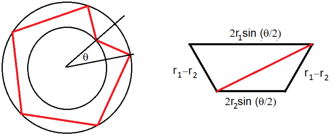
Refer to caption
Figure 3: The energy of a magnon stretching between the two radii is determined by the length of the diagonal of the parallel trapezium shown.

An immediate test of this dilatation operator is to see if we obtain the expected anomalous dimension for each magnon. Consider a magnon stretching between two different radii r1>r2r_{1}>r_{2} on the LLM plane, as shown in Figure 3. The energy of the magnon stretching between the two radii is given in terms of the length of the diagonal of the parallel trapezium[43]. This length squared is given by Ptolemy’s theorem as

l2=(r1−r2)2+4​r1​r2​sin2⁡θ2\displaystyle l^{2}=(r_{1}-r_{2})^{2}+4r_{1}r_{2}\sin^{2}{\theta\over 2} (2.22)

The energy of the magnon is given by[43]

E=1+4​g2​l2=1+2​g2​l2+⋯\displaystyle E=\sqrt{1+4g^{2}l^{2}}=1+2g^{2}l^{2}+\cdots (2.23)

so that the one loop anomalous dimension is given by

γ=2​g2​((r1−r2)2+4​r1​r2​sin2⁡θ2)=2​g2​(r12+r22−2​r1​r2​cos⁡θ)\displaystyle\gamma=2g^{2}((r_{1}-r_{2})^{2}+4r_{1}r_{2}\sin^{2}{\theta\over 2})=2g^{2}(r_{1}^{2}+r_{2}^{2}-2r_{1}r_{2}\cos\theta) (2.24)

Writing this in terms of gauge theory parameters ri=ciNr_{i}=\sqrt{\frac{c_{i}}{N}} we have

γ=2​g2​(c1N+c2N−2​c1​c2N​cos⁡p)\displaystyle\gamma=2g^{2}\left({c_{1}\over N}+{c_{2}\over N}-2{\sqrt{c_{1}c_{2}}\over N}\cos p\right) (2.25)

in complete harmony with our discussion above.

3 Magnon Scattering

The SS-matrix for two magnon scattering is completely determined, up to a phase, by the s​u​(2|2)2su(2|2)^{2} symmetry that our subsector enjoys[11]. In the next subsection we will obtain this two magnon scattering matrix, for the general case that the magnons that scatter stretch between different ring edges on the LLM plane. As a perturbative test of this result, we expand the SS-matrix in a weak coupling expansion and demonstrate agreement with one and two loop magnon scattering in the CFT.

A remark is in order. In determining the SS-matrix up to a phase we have not made any use of integrability. The only input is the s​u​(2|2)2su(2|2)^{2} symmetry that our operators enjoy. This symmetry is present whenever we deal with operators constructed using many ZZs and then doped with a much smaller number of impurities. This includes, for example, open strings attached to giant gravitons as well as closed string excitations of LLM geometries.

3.1 The Exact Two-magnon S-matrix

The parameters determining the kinematical state of a magnon stretching from radius rir_{i} to radius rjr_{j} with momentum pp are

xi±\displaystyle x_{i}^{\pm} =\displaystyle= i​e±i​pi2​(1+Ei)2​g​(ri​ei​pi2−rj​e−i​pi2)\displaystyle\frac{ie^{\pm i\frac{p_{i}}{2}}(1+E_{i})}{2g(r_{i}e^{i\frac{p_{i}}{2}}-r_{j}e^{-i\frac{p_{i}}{2}})}
Ei\displaystyle E_{i} =\displaystyle= 1+4​g2​(ri2+rj2)−8​g2​ri​rj​cos⁡(pi)\displaystyle\sqrt{1+4g^{2}(r_{i}^{2}+r_{j}^{2})-8g^{2}r_{i}r_{j}\cos(p_{i})} (3.1)

They satisfy the following conditions

ri​xi++rixi+−rj​xi−−rjxi−\displaystyle r_{i}x_{i}^{+}+\frac{r_{i}}{x_{i}^{+}}-r_{j}x_{i}^{-}-\frac{r_{j}}{x_{i}^{-}} =\displaystyle= ig\displaystyle\frac{i}{g} (3.2)
xi+xi−\displaystyle\frac{x_{i}^{+}}{x_{i}^{-}} =\displaystyle= ei​pi\displaystyle e^{ip_{i}} (3.3)

The magnon 1 has its end points on rings with radii r0r_{0} and r1r_{1}, while magnon 2 has its end points on rings with radii r0r_{0} and r2r_{2}. To specify the s​u​(2|2)su(2|2) representation that each magnon transforms in, following [11], we specify parameters ak,bk,ck,dka_{k},b_{k},c_{k},d_{k}, where

Qaα​|ϕb⟩=ak​δab​|ψα⟩,Qaα​|ψβ⟩=bk​ϵα​β​ϵa​b​|ϕb⟩,\displaystyle Q^{\alpha}_{a}|\phi^{b}\rangle=a_{k}\delta_{a}^{b}|\psi^{\alpha}\rangle\,,\qquad Q^{\alpha}_{a}|\psi^{\beta}\rangle=b_{k}\epsilon^{\alpha\beta}\epsilon_{ab}|\phi^{b}\rangle\,, (3.4)
Sαa​|ϕb⟩=ck​ϵα​β​ϵa​b​|ψβ⟩,Sαa​|ψβ⟩=dk​δαβ​|ϕa⟩,\displaystyle S^{a}_{\alpha}|\phi^{b}\rangle=c_{k}\epsilon_{\alpha\beta}\epsilon^{ab}|\psi^{\beta}\rangle\,,\qquad S^{a}_{\alpha}|\psi^{\beta}\rangle=d_{k}\delta^{\beta}_{\alpha}|\phi^{a}\rangle\,, (3.5)

for the kkth magnon. The representation for magnon 1 is defined by

a1=g​r0​η1,b1=g​r0η1​α1​f1​(1−r1r0​x1+x1−)\displaystyle a_{1}=\sqrt{gr_{0}}\eta_{1}\,,\qquad b_{1}={\sqrt{gr_{0}}\over\eta_{1}}\alpha_{1}f_{1}\left(1-\frac{r_{1}}{r_{0}}{x^{+}_{1}\over x^{-}_{1}}\right) (3.6)
c1=g​r0​i​η1α1​f1​x1+,d1=g​r0​x1+i​η1​(1−r1r0​x1−x1+)\displaystyle c_{1}={\sqrt{gr_{0}}i\eta_{1}\over\alpha_{1}f_{1}x^{+}_{1}}\,,\qquad d_{1}={\sqrt{gr_{0}}x^{+}_{1}\over i\eta_{1}}\left(1-\frac{r_{1}}{r_{0}}{x^{-}_{1}\over x^{+}_{1}}\right) (3.7)

and the representation for magnon 2 by

a2=g​r0​η2,b2=g​r0η2​α2​f2​(1−r2r0​x2+x2−)\displaystyle a_{2}=\sqrt{gr_{0}}\eta_{2}\,,\qquad b_{2}={\sqrt{gr_{0}}\over\eta_{2}}\alpha_{2}f_{2}\left(1-\frac{r_{2}}{r_{0}}{x_{2}^{+}\over x_{2}^{-}}\right) (3.8)
c2=g​r0​i​η2α2​f2​x2+,d2=g​r0​x2+i​η2​(1−r2r0​x2−x2+).\displaystyle c_{2}={\sqrt{gr_{0}}i\eta_{2}\over\alpha_{2}f_{2}x_{2}^{+}}\,,\qquad d_{2}={\sqrt{gr_{0}}x_{2}^{+}\over i\eta_{2}}\left(1-\frac{r_{2}}{r_{0}}{x_{2}^{-}\over x_{2}^{+}}\right)\,. (3.9)

fif_{i} is the product of ∏kei​pk\prod_{k}e^{ip_{k}} for all the magnons to the left of the one considered. The αi\alpha_{i}’s are phases that position the endpoints of the magnon on the LLM plane. Denote the magnons before scattering with 1 and 2 and after the scattering with 1′1^{\prime} and 2′2^{\prime}. We have

α1\displaystyle\alpha_{1} =\displaystyle= r0​x1+−r1​x1−r1​x1+−r0​x1−​α2α1′=r0​x1′+−r1​x1′−r1​x1′+−r0​x1′−​α2α2′=α2.\displaystyle\frac{r_{0}x_{1}^{+}-r_{1}x_{1}^{-}}{r_{1}x_{1}^{+}-r_{0}x_{1}^{-}}\alpha_{2}\qquad\alpha_{1^{\prime}}=\frac{r_{0}x_{1^{\prime}}^{+}-r_{1}x_{1^{\prime}}^{-}}{r_{1}x_{1^{\prime}}^{+}-r_{0}x_{1^{\prime}}^{-}}\alpha_{2}\qquad\alpha_{2^{\prime}}=\alpha_{2}. (3.10)

The SS-matrix is now determined, following [11], by using the magnon representation given above and requiring that the SS-matrix commutes with the elements of s​u​(2|2)su(2|2). We will focus on an initial state of two bosonic magnons

S12|ϕ1aϕ2b⟩=A12|ϕ2′{aϕ1′b}⟩+B12|ϕ2′[aϕ1′b]⟩+12C12ϵa​bϵα​β|ψ2′αψ1′β⟩\displaystyle S_{12}|\phi_{1}^{a}\phi_{2}^{b}\rangle=A_{12}|\phi_{2^{\prime}}^{\{a}\phi_{1^{\prime}}^{b\}}\rangle+B_{12}|\phi_{2^{\prime}}^{[a}\phi_{1^{\prime}}^{b]}\rangle+{1\over 2}C_{12}\epsilon^{ab}\epsilon_{\alpha\beta}|\psi_{2^{\prime}}^{\alpha}\psi_{1^{\prime}}^{\beta}\rangle (3.11)

The resulting S-matrix elements are given by

A12\displaystyle A_{12} =\displaystyle= S120​NA12DA12\displaystyle S^{0}_{12}\frac{N_{A_{12}}}{D_{A_{12}}}
NA12\displaystyle N_{A_{12}} =\displaystyle= −x1−​x2−​(−x1−​(x1++x2+)+r1r0​((x1−)2+x1+​x2+))​(r1r0​x1′⁣−−x1′⁣+)​x1′⁣+​x2′⁣+​η1​η2\displaystyle-x_{1}^{-}x_{2}^{-}(-x_{1}^{-}(x_{1}^{+}+x_{2}^{+})+\frac{r_{1}}{r_{0}}((x_{1}^{-})^{2}+x_{1}^{+}x_{2}^{+}))(\frac{r_{1}}{r_{0}}x_{1}^{\prime-}-x_{1}^{\prime+})x_{1}^{\prime+}x_{2}^{\prime+}\eta_{1}\eta_{2}
DA12\displaystyle D_{A_{12}} =\displaystyle= (r1r0​x1−−x1+)​x1′⁣−​(−x1−​x2−​(x1++x2+)​x1′⁣+​x2′⁣++CLOSE\displaystyle(\frac{r_{1}}{r_{0}}x_{1}^{-}-x_{1}^{+})x_{1}^{\prime-}\left(-x_{1}^{-}x_{2}^{-}(x_{1}^{+}+x_{2}^{+})x_{1}^{\prime+}x_{2}^{\prime+}+\right.
OPEN+r1r0​x1+​x2−​x2+​(x1−​x1′⁣−+x1′⁣+​x2′⁣+)+r2r0​x1+​x2+​(−x1+​x2+​x1′⁣−+x1−​x1′⁣+​x2′⁣+))​η1′​η2′\displaystyle+\left.\frac{r_{1}}{r_{0}}x_{1}^{+}x_{2}^{-}x_{2}^{+}(x_{1}^{-}x_{1}^{\prime-}+x_{1}^{\prime+}x_{2}^{\prime+})+\frac{r_{2}}{r_{0}}x_{1}^{+}x_{2}^{+}(-x_{1}^{+}x_{2}^{+}x_{1}^{\prime-}+x_{1}^{-}x_{1}^{\prime+}x_{2}^{\prime+})\right)\eta_{1}^{\prime}\eta_{2}^{\prime}
B12\displaystyle B_{12} =\displaystyle= S120​NB12DB12\displaystyle S^{0}_{12}\frac{N_{B_{12}}}{D_{B_{12}}}
DB12\displaystyle D_{B_{12}} =\displaystyle= (r1r0​x1−​x2−−r2r0​x1+​x2+)​(r1r0​x1′⁣−​x2′⁣−−r2r0​x1′⁣+​x2′⁣+)​DA12\displaystyle(\frac{r_{1}}{r_{0}}x_{1}^{-}x_{2}^{-}-\frac{r_{2}}{r_{0}}x_{1}^{+}x_{2}^{+})(\frac{r_{1}}{r_{0}}x_{1}^{\prime-}x_{2}^{\prime-}-\frac{r_{2}}{r_{0}}x_{1}^{\prime+}x_{2}^{\prime+})D_{A_{12}}
NB12\displaystyle N_{B_{12}} =\displaystyle= −x1−x2−(r1r0x1′⁣−−x1′⁣+)x1′⁣+[4(r1r0x1−−x1+)x1+x2+(r1r0x1−x2−−r2r0x1+x2+)x1′⁣−x2′⁣−+\displaystyle-x_{1}^{-}x_{2}^{-}(\frac{r_{1}}{r_{0}}x_{1}^{\prime-}-x_{1}^{\prime+})x_{1}^{\prime+}\left[4(\frac{r_{1}}{r_{0}}x_{1}^{-}-x_{1}^{+})x_{1}^{+}x_{2}^{+}(\frac{r_{1}}{r_{0}}x_{1}^{-}x_{2}^{-}-\frac{r_{2}}{r_{0}}x_{1}^{+}x_{2}^{+})x_{1}^{\prime-}x_{2}^{\prime-}+\right. (3.12)
+(4​r2r0​(r1r0​x1−−x1+)​x1+​x2+​(−r1r0​x1−​x2−+r2r0​x1+​x2+)​x1′⁣−+CLOSE\displaystyle+\left.(4\frac{r_{2}}{r_{0}}(\frac{r_{1}}{r_{0}}x_{1}^{-}-x_{1}^{+})x_{1}^{+}x_{2}^{+}(-\frac{r_{1}}{r_{0}}x_{1}^{-}x_{2}^{-}+\frac{r_{2}}{r_{0}}x_{1}^{+}x_{2}^{+})x_{1}^{\prime-}+\right.
+(r1r0​(r1r0​x1−​x2−−2​x1+​x2−+r2r0​x1+​x2+)​(−x1−​(x1++x2+)+r1r0​((x1−)2+x1+​x2+))​x1′⁣−−CLOSE\displaystyle+\left.(\frac{r_{1}}{r_{0}}(\frac{r_{1}}{r_{0}}x_{1}^{-}x_{2}^{-}-2x_{1}^{+}x_{2}^{-}+\frac{r_{2}}{r_{0}}x_{1}^{+}x_{2}^{+})(-x_{1}^{-}(x_{1}^{+}+x_{2}^{+})+\frac{r_{1}}{r_{0}}((x_{1}^{-})^{2}+x_{1}^{+}x_{2}^{+}))x_{1}^{\prime-}-\right.
OPENOPEN−2​(r1r0​x1−​x2−−r2r0​x1+​x2+)​(x1−​(−x1++x2+)+r1r0​((x1−)2−x1+​x2+))​x1′⁣+)​x2′⁣−)​x2′⁣++\displaystyle\left.-2(\frac{r_{1}}{r_{0}}x_{1}^{-}x_{2}^{-}-\frac{r_{2}}{r_{0}}x_{1}^{+}x_{2}^{+})(x_{1}^{-}(-x_{1}^{+}+x_{2}^{+})+\frac{r_{1}}{r_{0}}((x_{1}^{-})^{2}-x_{1}^{+}x_{2}^{+}))x_{1}^{\prime+})x_{2}^{\prime-})x_{2}^{\prime+}+\right.
r2r0(x1−(r1r0x1−−x1+)(r1r0x1−+2x1+)x2−+(3r2r0x1−x1+(−r1r0x1−+x1+)+(3r1r0x1−−\displaystyle\left.\frac{r_{2}}{r_{0}}(x_{1}^{-}(\frac{r_{1}}{r_{0}}x_{1}^{-}-x_{1}^{+})(\frac{r_{1}}{r_{0}}x_{1}^{-}+2x_{1}^{+})x_{2}^{-}+(3\frac{r_{2}}{r_{0}}x_{1}^{-}x_{1}^{+}(-\frac{r_{1}}{r_{0}}x_{1}^{-}+x_{1}^{+})+(3\frac{r_{1}}{r_{0}}x_{1}^{-}-\right.
−2x1+)(x1−−r1r0x1+)x2−)x2++r2r0x1+(−x1−+r1r0x1+)(x2+)2)x1′⁣+(x2′⁣+)2]η1η2\displaystyle\left.-2x_{1}^{+})(x_{1}^{-}-\frac{r_{1}}{r_{0}}x_{1}^{+})x_{2}^{-})x_{2}^{+}+\frac{r_{2}}{r_{0}}x_{1}^{+}(-x_{1}^{-}+\frac{r_{1}}{r_{0}}x_{1}^{+})(x_{2}^{+})^{2})x_{1}^{\prime+}(x_{2}^{\prime+})^{2}\right]\eta_{1}\eta_{2}

where S120S^{0}_{12} is an overall phase of the S-matrix, not determined by the symmetry argument. The initial and final energies and momenta are related by the usual conservation laws

E1+E2−E1′−E2′=0=p1+p2−p1′−p2′E_{1}+E_{2}-E_{1}^{\prime}-E_{2}^{\prime}=0=p_{1}+p_{2}-p_{1}^{\prime}-p_{2}^{\prime} (3.13)

which fixes the values for p1′p_{1}^{\prime} and p2′p_{2}^{\prime} uniquely.

3.2 One-loop

Our analysis in this subsection follows [42]. The reader may wish to consult this paper for further background. We treat the dilatation operator as a Hamiltonian, and study the resulting problem of magnon scattering. Introduce the wave function ψ⁡(l1,l2,⋯)\psi(l_{1},l_{2},\cdots) as follows

O=∑l0,l1,l2,⋯ψ⁡(l1,l2,⋯)​OB​((l0)0,(l1,…)1,(l2,⋯)2,⋯).\displaystyle O=\sum_{l_{0},l_{1},l_{2},\cdots}\psi(l_{1},l_{2},\cdots)O_{B}((l_{0})_{0},(l_{1},...)_{1},(l_{2},\cdots)_{2},\cdots)\,. (3.14)

The magnons at l1l_{1} (magnon 1) and l2l_{2} (magnon 2) meet at the edge of an annulus of radius squared r02=coNr_{0}^{2}={c_{o}\over N}. Magnon 11 stretches to the edge of an annulus of radius squared r12=c1Nr_{1}^{2}={c_{1}\over N} and magnon 22 to the edge of an annulus of radius squared r22=c2Nr_{2}^{2}={c_{2}\over N}. We do not assume any ordering of c0,c1c_{0},c_{1} and c2c_{2}. These two magnons are well separated from the remaining magnons (so we can consider them on their own) and are both taken to be YY impurities, which is general enough for our study. The time independent Schrödinger equation following from the one loop dilatation operator is

E​ψ​(l1,l2)=(2​r02+r12+r22)​ψ​(l1,l2)−r0​r1​(ψ⁡(l1−1,l2)+ψ⁡(l1+1,l2))\displaystyle E\psi(l_{1},l_{2})=\left(2r_{0}^{2}+r_{1}^{2}+r_{2}^{2}\right)\psi(l_{1},l_{2})-r_{0}r_{1}\left(\psi(l_{1}-1,l_{2})+\psi(l_{1}+1,l_{2})\right) (3.15)
−r0​r2​(ψ⁡(l1,l2−1)+ψ⁡(l1,l2+1))\displaystyle-r_{0}r_{2}(\psi(l_{1},l_{2}-1)+\psi(l_{1},l_{2}+1)) (3.16)

The equation (3.16) is valid whenever the magnons are not adjacent in the string word, i.e. when l2>l1+1l_{2}>l_{1}+1. If the magnons are adjacent, we find

E​ψ​(l1,l1+1)=(r12+r22)​ψ​(l1,l1+1)−r0​r1​ψ​(l1−1,l1+1)−r0​r2​ψ​(l1,l1+2).\displaystyle E\psi(l_{1},l_{1}+1)=\left(r_{1}^{2}+r_{2}^{2}\right)\psi(l_{1},l_{1}+1)-r_{0}r_{1}\psi(l_{1}-1,l_{1}+1)-r_{0}r_{2}\psi(l_{1},l_{1}+2)\,. (3.17)

Make the following Bethe ansatz for the wave function

ψ⁡(l1,l2)=ei​p1​l1+i​p2​l2+R12​ei​p1′​l1+i​p2′​l2.\displaystyle\psi(l_{1},l_{2})=e^{ip_{1}l_{1}+ip_{2}l_{2}}+R_{12}\,e^{ip_{1}^{\prime}l_{1}+ip_{2}^{\prime}l_{2}}\,. (3.18)

It is straight forward to see that this ansatz obeys (3.16) as long as

E=2​r02+r12+r22−r0​r1​(ei​p1+e−i​p1)−r0​r2​(ei​p2+e−i​p2)\displaystyle E=2r_{0}^{2}+r_{1}^{2}+r_{2}^{2}-r_{0}r_{1}(e^{ip_{1}}+e^{-ip_{1}})-r_{0}r_{2}(e^{ip_{2}}+e^{-ip_{2}}) (3.19)

and

r0​r1​(ei​p1+e−i​p1)+r0​r2​(ei​p2+e−i​p2)=r0​r1​(ei​p1′+e−i​p1′)+r0​r2​(ei​p2′+e−i​p2′).\displaystyle r_{0}r_{1}(e^{ip_{1}}+e^{-ip_{1}})+r_{0}r_{2}\left(e^{ip_{2}}+e^{-ip_{2}}\right)=r_{0}r_{1}(e^{ip_{1}^{\prime}}+e^{-ip_{1}^{\prime}})+r_{0}r_{2}\left(e^{ip_{2}^{\prime}}+e^{-ip_{2}^{\prime}}\right)\,. (3.20)

Note that (3.19) is indeed the correct one loop anomalous dimension and (3.20) can be obtained by equating the O⁡(λ)O(\lambda) terms in the equation expressing the conservation of magnon energies. From (3.17) we can solve for the reflection coefficient R12R_{12}. The result is

R12=−2​ei​p2−r1r0​ei​p1+i​p2−r2r02​ei​p2′−r1r0​ei​p1′+i​p2′−r2r0\displaystyle R_{12}=-{2e^{ip_{2}}-\frac{r_{1}}{r_{0}}e^{ip_{1}+ip_{2}}-\frac{r_{2}}{r_{0}}\over 2e^{ip_{2}^{\prime}}-\frac{r_{1}}{r_{0}}e^{ip_{1}^{\prime}+ip_{2}^{\prime}}-\frac{r_{2}}{r_{0}}} (3.21)

This is a rather simple result. Two easy checks are

  • 1.

    We see that R12​R21=1R_{12}R_{21}=1.

  • 2.

    If we set r1=r2=r0=1r_{1}=r_{2}=r_{0}=1 we recover the S-matrix of [42]. If we set r0=r2=Nr_{0}=r_{2}=N and keep r1r_{1} arbitrary, we recover the result of [12].

To continue we need to go beyond the s​u​(2)su(2) sector by considering a state with a single YY impurity and a single XX impurity. The operator with a YY impurity at l1l_{1} (this is now magnon 1) and an XX impurity at l2l_{2} (this is now magnon 2) is denoted OB​((l0)0,(l1,…)1,(l2,⋯)2,⋯)Y​XO_{B}((l_{0})_{0},(l_{1},...)_{1},(l_{2},\cdots)_{2},\cdots)_{YX} and the operator with an XX impurity at l1l_{1} (magnon 1) and a YY impurity at l2l_{2} (magnon 2) is denoted OB​((l0)0,(l1,…)1,(l2,⋯)2,⋯)X​YO_{B}((l_{0})_{0},(l_{1},...)_{1},(l_{2},\cdots)_{2},\cdots)_{XY}. Introduce the pair of wave functions

O=∑l1,l2,⋯[ψY​X(l1,l2,⋯)OB((l0)0,(l1,…)1,(l2,⋯)2,⋯)Y​X\displaystyle O=\sum_{l_{1},l_{2},\cdots}\left[\psi_{YX}(l_{1},l_{2},\cdots)O_{B}((l_{0})_{0},(l_{1},...)_{1},(l_{2},\cdots)_{2},\cdots)_{YX}\right. (3.22)
+ψX​Y(l1,l2,⋯)OB((l0)0,(l1,…)1,(l2,⋯)2,⋯)X​Y].\displaystyle\left.+\psi_{XY}(l_{1},l_{2},\cdots)O_{B}((l_{0})_{0},(l_{1},...)_{1},(l_{2},\cdots)_{2},\cdots)_{XY}\right]\,. (3.23)

We find the time independent Schrödinger equation (3.16) for each wave function, when the impurities are not adjacent. When the impurities are adjacent, we find

E​ψA​B​(l1,l1+1)=(r02+r12+r22)​ψA​B​(l1,l1+1)−r0​r1​ψA​B​(l1−1,l1+1)\displaystyle E\psi_{AB}(l_{1},l_{1}+1)=\left(r_{0}^{2}+r_{1}^{2}+r_{2}^{2}\right)\psi_{AB}(l_{1},l_{1}+1)-r_{0}r_{1}\psi_{AB}(l_{1}-1,l_{1}+1) (3.24)
−r02​ψB​A​(l1,l1+1)−r0​r2​ψA​B​(l1,l1+2)\displaystyle-r_{0}^{2}\psi_{BA}(l_{1},l_{1}+1)-r_{0}r_{2}\psi_{AB}(l_{1},l_{1}+2) (3.25)

where AA and BB could be either XX or YY. Make the following Bethe ansatz for the wave function

ψY​X​(l1,l2)=ei​p1​l1+i​p2​l2+A​ei​p1′​l1+i​p2′​l2ψX​Y​(l1,l2)=B​ei​p1′​l1+i​p2′​l2\displaystyle\psi_{YX}(l_{1},l_{2})=e^{ip_{1}l_{1}+ip_{2}l_{2}}+Ae^{ip_{1}^{\prime}l_{1}+ip_{2}^{\prime}l_{2}}\qquad\psi_{XY}(l_{1},l_{2})=Be^{ip_{1}^{\prime}l_{1}+ip_{2}^{\prime}l_{2}} (3.26)

The two equations of the form (3.16) imply that both ψX​Y​(l1,l2)\psi_{XY}(l_{1},l_{2}) and ψY​X​(l1,l2)\psi_{YX}(l_{1},l_{2}) have the same energy, which is given in (3.19). The equations (3.25) imply that

A=ei​p2′+ei​p2−r2r0−r1r0​ei​p2′+i​p1′r2r0+r1r0​ei​p1′+i​p2′−2​ei​p2′B=ei​p2′−ei​p2r2r0+r1r0​ei​p1′+i​p2′−2​ei​p2′.\displaystyle A={e^{ip_{2}^{\prime}}+e^{ip_{2}}-\frac{r_{2}}{r_{0}}-\frac{r_{1}}{r_{0}}e^{ip_{2}^{\prime}+ip_{1}^{\prime}}\over\frac{r_{2}}{r_{0}}+\frac{r_{1}}{r_{0}}e^{ip_{1}^{\prime}+ip_{2}^{\prime}}-2e^{ip_{2}^{\prime}}}\qquad B={e^{ip_{2}^{\prime}}-e^{ip_{2}}\over\frac{r_{2}}{r_{0}}+\frac{r_{1}}{r_{0}}e^{ip_{1}^{\prime}+ip_{2}^{\prime}}-2e^{ip_{2}^{\prime}}}\,. (3.27)

These again have a nice simple dependence on c0c_{0}, c1c_{1} and c2c_{2}. One can check that |A|2+|B|2=1|A|^{2}+|B|^{2}=1 which is a consequence of unitarity. To perform the check it is necessary to use the conservation of momentum p1+p2=p1′+p2′p_{1}+p_{2}=p_{1}^{\prime}+p_{2}^{\prime} and the constraint (3.20). We now obtain

AR12=ei​p2′+ei​p2−r2r0−r1r0​ei​p1′+i​p2′2​ei​p1−r2r0−r1r0​ei​p1+i​p2.\displaystyle{A\over R_{12}}={e^{ip_{2}^{\prime}}+e^{ip_{2}}-\frac{r_{2}}{r_{0}}-\frac{r_{1}}{r_{0}}e^{ip_{1}^{\prime}+ip_{2}^{\prime}}\over 2e^{ip_{1}}-\frac{r_{2}}{r_{0}}-\frac{r_{1}}{r_{0}}e^{ip_{1}+ip_{2}}}\,. (3.28)

This should be equal to

12​(1+B12A12)\displaystyle{1\over 2}\left(1+{B_{12}\over A_{12}}\right) (3.29)

where A12A_{12} and B12B_{12} are the exact S-matrix elements determined by the s​u​(2|2)2su(2|2)^{2} symmetry. We now expand the exact S-matrix in powers of gg and compare it with the above one-loop result. The first order expression is

A12\displaystyle A_{12} =\displaystyle= −2​ei​p2−r1r0​ei⁡(p1+p2)−r2r02​ei​p2′−r1r0​ei⁡(p1′+p2′)−r2r0×η1​η2η1′​η2′\displaystyle-\frac{2e^{ip_{2}}-\frac{r_{1}}{r_{0}}e^{i(p_{1}+p_{2})}-\frac{r_{2}}{r_{0}}}{2e^{ip_{2}^{\prime}}-\frac{r_{1}}{r_{0}}e^{i(p_{1}^{\prime}+p_{2}^{\prime})}-\frac{r_{2}}{r_{0}}}\times\frac{\eta_{1}\eta_{2}}{\eta_{1}^{\prime}\eta_{2}^{\prime}} (3.30)
12​(1+A12B12)\displaystyle\frac{1}{2}\left(1+\frac{A_{12}}{B_{12}}\right) =\displaystyle= −ei​p2′−ei​p2+r1r0​ei⁡(p1+p2)+r2r0−2​ei​p2+r1r0​ei⁡(p1+p2)+r2r0.\displaystyle\frac{-e^{ip_{2}^{\prime}}-e^{ip_{2}}+\frac{r_{1}}{r_{0}}e^{i(p_{1}+p_{2})}+\frac{r_{2}}{r_{0}}}{-2e^{ip_{2}}+\frac{r_{1}}{r_{0}}e^{i(p_{1}+p_{2})}+\frac{r_{2}}{r_{0}}}. (3.31)

There is complete agreement between (3.28) and (3.31).

3.3 Two loops

We now consider scattering to two loops. A similar computation for the s​u​(2)su(2) sector is considered in [44] to determine the energy and the scattering element R12R_{12} to two loops. At two loops R12R_{12} receives non-trivial contributions from the overall scattering phase. To carry out a check independent of the unknown scattering phase, we again compare ratios of SS-matrix elements. We can carry this out in the s​u​(2|3)su(2|3) sector of the theory. At two loops fermionic terms contribute. The various interaction terms in the dilatation operator up to two loops have been determined in [46]. For our study we begin by generalizing the existing result by adjusting the weights of the various terms.

Our initial state consists of two types of impuries so that only the following terms in the dilatation operator are relevant (we use the notation spelled out in [46])

D0\displaystyle D_{0} =\displaystyle= {aa}+32​{αα}\displaystyle\left\{\begin{array}[]{c}a\\ a\end{array}\right\}+\frac{3}{2}\left\{\begin{array}[]{c}\alpha\\ \alpha\end{array}\right\}
D2\displaystyle D_{2} =\displaystyle= α12​{abab}+α12​({aβaβ}+{αbαb})+α12​{αβαβ}\displaystyle\alpha_{1}^{2}\left\{\begin{array}[]{cc}a&b\\ a&b\end{array}\right\}+\alpha_{1}^{2}\left(\left\{\begin{array}[]{cc}a&\beta\\ a&\beta\end{array}\right\}+\left\{\begin{array}[]{cc}\alpha&b\\ \alpha&b\end{array}\right\}\right)+\alpha_{1}^{2}\left\{\begin{array}[]{cc}\alpha&\beta\\ \alpha&\beta\end{array}\right\}
−α12​{abba}−α12​({aββa}+{αbbα})+α12​{αββα}\displaystyle-\alpha_{1}^{2}\left\{\begin{array}[]{cc}a&b\\ b&a\end{array}\right\}-\alpha_{1}^{2}\left(\left\{\begin{array}[]{cc}a&\beta\\ \beta&a\end{array}\right\}+\left\{\begin{array}[]{cc}\alpha&b\\ b&\alpha\end{array}\right\}\right)+\alpha_{1}^{2}\left\{\begin{array}[]{cc}\alpha&\beta\\ \beta&\alpha\end{array}\right\}
D3\displaystyle D_{3} =\displaystyle= −12​α13​ei​β2​ϵα​β​ϵa​b​c​{αβabc}−12​α13​e−i​β2​ϵα​β​ϵa​b​c​{abcαβ}\displaystyle-\frac{1}{\sqrt{2}}\alpha_{1}^{3}e^{i\beta_{2}}\epsilon_{\alpha\beta}\epsilon^{abc}\left\{\begin{array}[]{ccccc}&\alpha&&\beta&\\ a&&b&&c\end{array}\right\}-\frac{1}{\sqrt{2}}\alpha_{1}^{3}e^{-i\beta_{2}}\epsilon^{\alpha\beta}\epsilon_{abc}\left\{\begin{array}[]{ccccc}a&&b&&c\\ &\alpha&&\beta&\end{array}\right\}
D4\displaystyle D_{4} =\displaystyle= (−2​α14+2​α1​α3)​({abcabc})+(32​α14−α1​α3)​({abcbac}+{abcacb})\displaystyle(-2\alpha_{1}^{4}+2\alpha_{1}\alpha_{3})\left(\left\{\begin{array}[]{ccc}a&b&c\\ a&b&c\end{array}\right\}\right)+(\frac{3}{2}\alpha_{1}^{4}-\alpha_{1}\alpha_{3})\left(\left\{\begin{array}[]{ccc}a&b&c\\ b&a&c\end{array}\right\}+\left\{\begin{array}[]{ccc}a&b&c\\ a&c&b\end{array}\right\}\right)
−12​α4​({abcbca}+{abccab})\displaystyle-\frac{1}{2}\alpha^{4}\left(\left\{\begin{array}[]{ccc}a&b&c\\ b&c&a\end{array}\right\}+\left\{\begin{array}[]{ccc}a&b&c\\ c&a&b\end{array}\right\}\right)

where a,ba,b and cc are any of the bosonic scalar fields and α\alpha, β\beta are any of the fermionic fields of the s​u​(2|3)su(2|3) sector. D0D_{0} is the classical dilatation operator, D2D_{2} a one loop contribution and D4D_{4} a two loop contribution. The term D3D_{3} which is of order gY​M3g_{YM}^{3} mixes operators with a different number of fields since it allows replacements of three boson fields with two fermion fields and vice versa. Using the results developed in section 22 we can adjust the weights of the various terms appearing in the dilatation operator, based on the local factors for the magnons involved. These weights are spelled out in our Bethe ansatz equations below. We set α1=2​gN\alpha_{1}=\frac{\sqrt{2}g}{\sqrt{N}} and α3=0\alpha_{3}=0. Factors of NN are absorbed by replacing ci→ri\sqrt{c_{i}}\rightarrow r_{i}.

We use ψA​B\psi_{AB} for a wave function with AA and BB bosonic excitations (AA and BB could be either XX or YY) and ψa​b\psi_{ab} for a wave function with fermionic excitations. When the magnons are well separated l2>l1+2l_{2}>l_{1}+2 we find

E​ψA​B​(l1,l2)\displaystyle E\psi_{AB}(l_{1},l_{2}) (3.72)
=\displaystyle= 2​g2​(2​r02+r12+r22)​ψA​B​(l1,l2)\displaystyle 2g^{2}\left(2r_{0}^{2}+r_{1}^{2}+r_{2}^{2}\right)\psi_{AB}(l_{1},l_{2})
−2​g2​r0​r1​(ψA​B​(l1−1,l2)+ψA​B​(l1+1,l2))−2​g2​r0​r2​(ψA​B​(l1,l2+1)+ψA​B​(l1,l2−1))\displaystyle-2g^{2}r_{0}r_{1}\left(\psi_{AB}(l_{1}-1,l_{2})+\psi_{AB}(l_{1}+1,l_{2})\right)-2g^{2}r_{0}r_{2}\left(\psi_{AB}(l_{1},l_{2}+1)+\psi_{AB}(l_{1},l_{2}-1)\right)
−2​g4​((r02+r12)2+(r02+r22)2)​ψA​B​(l1,l2)+4​g4​(r02+r12)​r0​r1​(ψA​B​(l1+1,l2)+ψA​B​(l1−1,l2))\displaystyle-2g^{4}\left((r_{0}^{2}+r_{1}^{2})^{2}+(r_{0}^{2}+r_{2}^{2})^{2}\right)\psi_{AB}(l_{1},l_{2})+4g^{4}\left(r_{0}^{2}+r_{1}^{2}\right)r_{0}r_{1}\left(\psi_{AB}(l_{1}+1,l_{2})+\psi_{AB}(l_{1}-1,l_{2})\right)
+4​g4​(r02+r22)​r0​r2​(ψA​B​(l1,l2+1)+ψA​B​(l1,l2−1))\displaystyle+4g^{4}\left(r_{0}^{2}+r_{2}^{2}\right)r_{0}r_{2}\left(\psi_{AB}(l_{1},l_{2}+1)+\psi_{AB}(l_{1},l_{2}-1)\right)
−2​g4​r02​r12​(ψA​B​(l1+2,l2)+2​ψA​B​(l1,l2)+ψA​B​(l1−2,l2))\displaystyle-2g^{4}r_{0}^{2}r_{1}^{2}\left(\psi_{AB}(l_{1}+2,l_{2})+2\psi_{AB}(l_{1},l_{2})+\psi_{AB}(l_{1}-2,l_{2})\right)
−2​g4​r02​r22​(ψA​B​(l1,l2+2)+2​ψA​B​(l1,l2)+ψA​B​(l1,l2−2))+o⁡(g6)\displaystyle-2g^{4}r_{0}^{2}r_{2}^{2}\left(\psi_{AB}(l_{1},l_{2}+2)+2\psi_{AB}(l_{1},l_{2})+\psi_{AB}(l_{1},l_{2}-2)\right)+o(g^{6})

When the magnons are seperated by two sites i.e. l2=l1+2l_{2}=l_{1}+2 we have

E​ψA​B​(l1,l1+2)\displaystyle E\psi_{AB}(l_{1},l_{1}+2) (3.73)
=\displaystyle= 2​g2​(2​r02+r12+r22)​ψA​B​(l1,l1+2)\displaystyle 2g^{2}\left(2r_{0}^{2}+r_{1}^{2}+r_{2}^{2}\right)\psi_{AB}(l_{1},l_{1}+2)
−2​g2​r0​r1​(ψA​B​(l1−1,l1+2)+ψA​B​(l1+1,l1+2))−2​g2​r0​r2​(ψA​B​(l1,l1+3)+ψA​B​(l1,l1+1))\displaystyle-2g^{2}r_{0}r_{1}\left(\psi_{AB}(l_{1}-1,l_{1}+2)+\psi_{AB}(l_{1}+1,l_{1}+2)\right)-2g^{2}r_{0}r_{2}\left(\psi_{AB}(l_{1},l_{1}+3)+\psi_{AB}(l_{1},l_{1}+1)\right)
−2​g4​((r02+r12)2+(r02+r22)2)​ψA​B​(l1,l1+2)\displaystyle-2g^{4}\left((r_{0}^{2}+r_{1}^{2})^{2}+(r_{0}^{2}+r_{2}^{2})^{2}\right)\psi_{AB}(l_{1},l_{1}+2)
+4​g4​(r02+r12)​r0​r1​(ψA​B​(l1+1,l1+2)+ψA​B​(l1−1,l1+2))\displaystyle+4g^{4}\left(r_{0}^{2}+r_{1}^{2}\right)r_{0}r_{1}\left(\psi_{AB}(l_{1}+1,l_{1}+2)+\psi_{AB}(l_{1}-1,l_{1}+2)\right)
+4​g4​(r02+r22)​r0​r2​(ψA​B​(l1,l1+3)+ψA​B​(l1,l1+1))\displaystyle+4g^{4}\left(r_{0}^{2}+r_{2}^{2}\right)r_{0}r_{2}\left(\psi_{AB}(l_{1},l_{1}+3)+\psi_{AB}(l_{1},l_{1}+1)\right)
−2​g4​r02​r12​(2​ψA​B​(l1,l1+2)+ψA​B​(l1−2,l1+2))\displaystyle-2g^{4}r_{0}^{2}r_{1}^{2}\left(2\psi_{AB}(l_{1},l_{1}+2)+\psi_{AB}(l_{1}-2,l_{1}+2)\right)
−2​g4​r02​r22​(ψA​B​(l1,l1+4)+2​ψA​B​(l1,l1+2))−4​r04​ψA​B​(l1,l1+2)\displaystyle-2g^{4}r_{0}^{2}r_{2}^{2}\left(\psi_{AB}(l_{1},l_{1}+4)+2\psi_{AB}(l_{1},l_{1}+2)\right)-4r_{0}^{4}\psi_{AB}(l_{1},l_{1}+2)
+2​g4​r02​(r0​r2​ψA​B​(l1,l1+1)+r0​r1​ψA​B​(l1+1,l1+2))\displaystyle+2g^{4}r_{0}^{2}\left(r_{0}r_{2}\psi_{AB}(l_{1},l_{1}+1)+r_{0}r_{1}\psi_{AB}(l_{1}+1,l_{1}+2)\right)
−2​g4​(r03​r2​ψB​A​(l1,l1+1)+r03​r1​ψB​A​(l1+1,l1+2))\displaystyle-2g^{4}(r_{0}^{3}r_{2}\psi_{BA}(l_{1},l_{1}+1)+r_{0}^{3}r_{1}\psi_{BA}(l_{1}+1,l_{1}+2))
−2​g3​r03​e−i​β​(−ψa​b​(l1,l1+1)+ψb​a​(l1,l1+1))+o⁡(g5)\displaystyle-2g^{3}r_{0}^{3}e^{-i\beta}(-\psi_{ab}(l_{1},l_{1}+1)+\psi_{ba}(l_{1},l_{1}+1))+o(g^{5})

and when they are adjacent i.e. l2=l1+1l_{2}=l_{1}+1

E​ψA​B​(l1,l1+1)\displaystyle E\psi_{AB}(l_{1},l_{1}+1) (3.74)
=\displaystyle= 2​g2​(r02+r12+r22)​ψA​B​(l1,l1+1)−2​g2​r0​r1​(ψA​B​(l1−1,l1+1))−g2​r0​r2​(ψA​B​(l1,l1+2))\displaystyle 2g^{2}\left(r_{0}^{2}+r_{1}^{2}+r_{2}^{2}\right)\psi_{AB}(l_{1},l_{1}+1)-2g^{2}r_{0}r_{1}\left(\psi_{AB}(l_{1}-1,l_{1}+1)\right)-g^{2}r_{0}r_{2}\left(\psi_{AB}(l_{1},l_{1}+2)\right)
−2​r02​g2​ψB​A​(l1,l1+1)\displaystyle-2r_{0}^{2}g^{2}\psi_{BA}(l_{1},l_{1}+1)
−2​g4​((r12+r02)2+(r22+r02)2)​ψA​B​(l1,l1+1)+4​g4​(r02+r12)​r0​r1​ψA​B​(l1−1,l1+1)\displaystyle-2g^{4}\left((r_{1}^{2}+r_{0}^{2})^{2}+(r_{2}^{2}+r_{0}^{2})^{2}\right)\psi_{AB}(l_{1},l_{1}+1)+4g^{4}(r_{0}^{2}+r_{1}^{2})r_{0}r_{1}\psi_{AB}(l_{1}-1,l_{1}+1)
+4​g4​(r02+r22)​r0​r2​ψA​B​(l1,l1+2)−2​g4​r02​r12​(ψA​B​(l1,l1+1)+ψA​B​(l1−2,l1+1))\displaystyle+4g^{4}(r_{0}^{2}+r_{2}^{2})r_{0}r_{2}\psi_{AB}(l_{1},l_{1}+2)-2g^{4}r_{0}^{2}r_{1}^{2}\left(\psi_{AB}(l_{1},l_{1}+1)+\psi_{AB}(l_{1}-2,l_{1}+1)\right)
−2​g4​r02​r22​(ψA​B​(l1,l1+1)+ψA​B​(l1,l1+3))−2​g4​r02​r1​r2​(ψA​B​(l1−1,l1)+ψA​B​(l1+1,l1+2))\displaystyle-2g^{4}r_{0}^{2}r_{2}^{2}\left(\psi_{AB}(l_{1},l_{1}+1)+\psi_{AB}(l_{1},l_{1}+3)\right)-2g^{4}r_{0}^{2}r_{1}r_{2}\left(\psi_{AB}(l_{1}-1,l_{1})+\psi_{AB}(l_{1}+1,l_{1}+2)\right)
−4​g4​(r02​ψB​A​(l1,l1+1))+2​g4​r03​r1​ψA​B​(l1−1,l1+1)+2​g4​r03​r2​ψA​B​(l1,l1+2)\displaystyle-4g^{4}\left(r_{0}^{2}\psi_{BA}(l_{1},l_{1}+1)\right)+2g^{4}r_{0}^{3}r_{1}\psi_{AB}(l_{1}-1,l_{1}+1)+2g^{4}r_{0}^{3}r_{2}\psi_{AB}(l_{1},l_{1}+2)
−2​g4​(r03​r1​ψB​A​(l1−1,l1+1)−2​(r04+r02​r12+r02​r22)​ψB​A​(l1,l1+1)+r03​r2​ψB​A​(l1,l1+2))\displaystyle-2g^{4}\left(r_{0}^{3}r_{1}\psi_{BA}(l_{1}-1,l_{1}+1)-2(r_{0}^{4}+r_{0}^{2}r_{1}^{2}+r_{0}^{2}r_{2}^{2})\psi_{BA}(l_{1},l_{1}+1)+r_{0}^{3}r_{2}\psi_{BA}(l_{1},l_{1}+2)\right)
−2​e−i​β​g3​r02​(r1​ψa​b​(l1−1,l1)+r2​ψa​b​(l1,l1+1)−r1​ψb​a​(l1−1,l1)−r2​ψb​a​(l1,l1+1)).\displaystyle-2e^{-i\beta}g^{3}r_{0}^{2}\left(r_{1}\psi_{ab}(l_{1}-1,l_{1})+r_{2}\psi_{ab}(l_{1},l_{1}+1)-r_{1}\psi_{ba}(l_{1}-1,l_{1})-r_{2}\psi_{ba}(l_{1},l_{1}+1)\right).

We also require the two-loop action on the fermionic excitations. When the fermionc excitations are adjacent we find

E​ψa​b​(l1,l1+1)\displaystyle E\psi_{ab}(l_{1},l_{1}+1) (3.75)
=\displaystyle= 2​g2​(r02+r12+r22)​ψa​b​(l1,l1+1)−2​g2​r0​r1​ψa​b​(l1−1,l1+1)−2​g2​r0​r2​ψa​b​(l1,l1+2)\displaystyle 2g^{2}(r_{0}^{2}+r_{1}^{2}+r_{2}^{2})\psi_{ab}(l_{1},l_{1}+1)-2g^{2}r_{0}r_{1}\psi_{ab}(l_{1}-1,l_{1}+1)-2g^{2}r_{0}r_{2}\psi_{ab}(l_{1},l_{1}+2)
+2​g2​r02​ψb​a​(l1,l1+1)\displaystyle+2g^{2}r_{0}^{2}\psi_{ba}(l_{1},l_{1}+1)
−2​g3​ei​β​r02​(r2​ψA​B​(l1,l1+1)−r2​ψB​A​(l1,l1+1)−r0​ψA​B​(l1,l1+2)CLOSE\displaystyle-2g^{3}e^{i\beta}r_{0}^{2}\left(r_{2}\psi_{AB}(l_{1},l_{1}+1)-r_{2}\psi_{BA}(l_{1},l_{1}+1)-r_{0}\psi_{AB}(l_{1},l_{1}+2)\right.
+r0​ψB​A​(l1,l1+2)+r1​ψA​B​(l1+1,l1+2)−r1​ψB​A​(l1+1)+o⁡(g5).\displaystyle+r_{0}\psi_{BA}(l_{1},l_{1}+2)+r_{1}\psi_{AB}(l_{1}+1,l_{1}+2)-r_{1}\psi_{BA}(l_{1}+1)+o(g^{5}).

To solve the above equations make the following Bethe ansatz [44, 47]

ψY​X​(l1,l2)\displaystyle\psi_{YX}(l_{1},l_{2}) =\displaystyle= ei​p1​l1+i​p2​l2+A​ei​p3​l1+i​p4​l2+r02​g2​δl2,l1+1​ϕY​X​(l1)\displaystyle e^{ip_{1}l_{1}+ip_{2}l_{2}}+Ae^{ip_{3}l_{1}+ip_{4}l_{2}}+r_{0}^{2}g^{2}\delta_{l_{2},l_{1}+1}\phi_{YX}(l_{1})
ψX​Y​(l1,l2)\displaystyle\psi_{XY}(l_{1},l_{2}) =\displaystyle= B​ei​p3​l1+i​p4​l2+r02​g2​δl2,l1+1​ϕX​Y​(l1)\displaystyle Be^{ip_{3}l_{1}+ip_{4}l_{2}}+r_{0}^{2}g^{2}\delta_{l_{2},l_{1}+1}\phi_{XY}(l_{1})
ψa​b​(l1,l2)\displaystyle\psi_{ab}(l_{1},l_{2}) =\displaystyle= g​C1​ei​p3​l1+i​p4​l2ψb​a​(l1,l2)=g​C2​ei​p3​l1+i​p4​l2.\displaystyle gC_{1}e^{ip_{3}l_{1}+ip_{4}l_{2}}\qquad\psi_{ba}(l_{1},l_{2})=gC_{2}e^{ip_{3}l_{1}+ip_{4}l_{2}}. (3.76)

Since we are working to two loops we can solve for p1′p_{1}^{\prime} and p2′p_{2}^{\prime} perturbatively to find

p1′\displaystyle p_{1}^{\prime} =\displaystyle= −ilog(ei​p2​(r1+ei​p1+i​p2​r2)ei​p1+i​p2​r1+r2+)+4g2r1r2(r12−r22)×\displaystyle-i\log\left(\frac{e^{ip_{2}}(r_{1}+e^{ip_{1}+ip_{2}}r_{2})}{e^{ip_{1}+ip_{2}}r_{1}+r_{2}}+\right)+4g^{2}r_{1}r_{2}(r_{1}^{2}-r_{2}^{2})\times
×e2​i​(p1+p2)​(r12+r22−2​r0​(r1​cos⁡(p1)+r2​cos⁡(p2))+2​r1​r2​cos⁡(p1+p2)(ei⁡(p1+p2)​r1+r2)2​(ei⁡(p1+p2)​r2+r1)2)​sin⁡(p1+p2)\displaystyle\times e^{2i(p_{1}+p_{2})}\left(\frac{r_{1}^{2}+r_{2}^{2}-2r_{0}(r_{1}\cos(p_{1})+r_{2}\cos(p_{2}))+2r_{1}r_{2}\cos(p_{1}+p_{2})}{(e^{i(p_{1}+p_{2})}r_{1}+r_{2})^{2}(e^{i(p_{1}+p_{2})}r_{2}+r_{1})^{2}}\right)\sin(p_{1}+p_{2})

and p2′=p1+p2−p1′p_{2}^{\prime}=p_{1}+p_{2}-p_{1}^{\prime}. Using these expressions and plugging our ansatz into the scattering equations we find

E\displaystyle E =\displaystyle= 2​(r02+r12−2​r0​r1​cos⁡(p1))​g2−2​(r02+r12−2​r0​r1​cos⁡(p1))2​g4\displaystyle 2(r_{0}^{2}+r_{1}^{2}-2r_{0}r_{1}\cos(p_{1}))g^{2}-2(r_{0}^{2}+r_{1}^{2}-2r_{0}r_{1}\cos(p_{1}))^{2}g^{4} (3.77)
+2​(r02+r22−2​r0​r2​cos⁡(p2))​g2−2​(r02+r22−2​r0​r2​cos⁡(p2))2​g4+o⁡(g5).\displaystyle+2(r_{0}^{2}+r_{2}^{2}-2r_{0}r_{2}\cos(p_{2}))g^{2}-2(r_{0}^{2}+r_{2}^{2}-2r_{0}r_{2}\cos(p_{2}))^{2}g^{4}+o(g^{5}).

which solves (3.72). This energy agrees with the exact expression to two loops. From (3.75) we determine C1C_{1} and C2C_{2} and from (3.73) we obtain ϕX​Y\phi_{XY} and ϕY​X\phi_{YX} in terms of AA and BB. These expressions, given in Appendix A, are cumbersome and are not quoted. Finally (3.74) determines AA and BB. The results are in Appendix A. In the end we obtain

A\displaystyle A =\displaystyle= ei​p2​r0​r1+ei⁡(2​p1+p2)​r0​r1+ei​p1​r0​r2+ei⁡(p1+2​p2)​r0​r2−r1​r2−e2​i​(p1+p2)​r1​r2−ei⁡(p1+p2)​(r12+r22)(ei⁡(p1+p2)​r1+r2)​(−2​ei​p1​r0+r1+ei⁡(p1+p2)​r2)\displaystyle\frac{e^{ip_{2}}r_{0}r_{1}+e^{i(2p_{1}+p_{2})}r_{0}r_{1}+e^{ip_{1}}r_{0}r_{2}+e^{i(p_{1}+2p_{2})}r_{0}r_{2}-r_{1}r_{2}-e^{2i(p_{1}+p_{2})}r_{1}r_{2}-e^{i(p_{1}+p_{2})}(r_{1}^{2}+r_{2}^{2})}{(e^{i(p_{1}+p_{2})}r_{1}+r_{2})(-2e^{ip_{1}}r_{0}+r_{1}+e^{i(p_{1}+p_{2})}r_{2})} (3.78)
+2​eOPEN−i⁡(p1+p2))​r0​NADA​g2+o⁡(g4)\displaystyle+2e^{-i(p_{1}+p_{2}))}r_{0}\frac{N_{A}}{D_{A}}g^{2}+o(g^{4})

and

B=r0​(ei​p2​r1−ei⁡(2​p1+p2)​r1−ei​p1​r2+ei⁡(p1+2​p2)​r2CLOSE(ei⁡(p1+p2)​r1+r2)​(−2​ei​p1​r0+r1+ei⁡(p1+p2)​r2)−2​e−i​p2​r0​NBDA​g2+o⁡(g4)B=\frac{r_{0}(e^{ip_{2}}r_{1}-e^{i(2p_{1}+p_{2})}r_{1}-e^{ip_{1}}r_{2}+e^{i(p_{1}+2p_{2})}r_{2}}{(e^{i(p_{1}+p_{2})}r_{1}+r_{2})(-2e^{ip_{1}}r_{0}+r_{1}+e^{i(p_{1}+p_{2})}r_{2})}-2e^{-ip_{2}}r_{0}\frac{N_{B}}{D_{A}}g^{2}+o(g^{4}) (3.79)

When r0=r1=r2=1r_{0}=r_{1}=r_{2}=1 we recover the scattering matrix of [11] and when r0=r1=1r_{0}=r_{1}=1 we recover the scattering matrix of [44]. We now find

AA+B=12​(1+B12A12)\frac{A}{A+B}=\frac{1}{2}\left(1+\frac{B_{12}}{A_{12}}\right) (3.80)

for any choice of r1,r2r_{1},r_{2} and r0r_{0}. This demonstrates that our SS-matrix agrees with the CFT scattering to two loops.

When r1=r2=r0r_{1}=r_{2}=r_{0} we find the simpler expressions

A\displaystyle A =\displaystyle= −(−1+ei​p1)​(−1+ei​p2)1−2​ei​p1+ei⁡(p1+p2)\displaystyle-\frac{(-1+e^{ip_{1}})(-1+e^{ip_{2}})}{1-2e^{ip_{1}}+e^{i(p_{1}+p_{2})}}
+2​e−i⁡(p1+p2)​(−1+ei​p1)2​(−1+ei​p2)2​(−ei​p1+e2​i​p1+ei​p2−ei⁡(p1+p2)−ei⁡(2​p1+p2)+ei⁡(p1+2​p2))​r02​g2(1−2​ei​p1+ei⁡(p1+p2))2\displaystyle+\frac{2e^{-i(p_{1}+p_{2})}(-1+e^{ip_{1}})^{2}(-1+e^{ip_{2}})^{2}(-e^{ip_{1}}+e^{2ip_{1}}+e^{ip_{2}}-e^{i(p_{1}+p_{2})}-e^{i(2p_{1}+p_{2})}+e^{i(p_{1}+2p_{2})})r_{0}^{2}g^{2}}{(1-2e^{ip_{1}}+e^{i(p_{1}+p_{2})})^{2}}
B\displaystyle B =\displaystyle= −ei​p1+ei​p21−2​ei​p1+ei⁡(p1+p2)+2​e−i​p2​(−1+ei​p1)2​(−1+ei​p2)2​(−ei​p1+ei​p2)​r02​g2(1−2​ei​p1+ei⁡(p1+p2))2.\displaystyle\frac{-e^{ip_{1}}+e^{ip_{2}}}{1-2e^{ip_{1}}+e^{i(p_{1}+p_{2})}}+\frac{2e^{-ip_{2}}(-1+e^{ip_{1}})^{2}(-1+e^{ip_{2}})^{2}(-e^{ip_{1}}+e^{ip_{2}})r_{0}^{2}g^{2}}{(1-2e^{ip_{1}}+e^{i(p_{1}+p_{2})})^{2}}. (3.81)

These S-matrices are related to those of [11] by rescaling g2→g2​r02g^{2}\rightarrow g^{2}r_{0}^{2}, as predicted in [7].

4 Finite Size Corrections

We now develop the string theory description of the gauge theory magnons. This probes the strong coupling limit of the magnon dynamics. We will compute corrections to the energy of magnons that carry finite angular momentum. As explained in the introduction, these finite size corrections are not determined by the s​u​(2|2)2su(2|2)^{2} symmetry of the problem.

We study classical string solutions on the {t,r,ϕ}\left\{t,r,\phi\right\} subspace of an LLM background

d​s2\displaystyle ds^{2} =\displaystyle= (r2​h2​(r)−h−2​(r)​(1+Vϕ​(r))2)​d​t2+2​(r2​h2​(r)−2​Vϕ​h−2​(r)​(1+Vϕ​(r)))​d​ϕ​d​t\displaystyle\left(r^{2}h^{2}(r)-h^{-2}(r)(1+V_{\phi}(r))^{2}\right)dt^{2}+2(r^{2}h^{2}(r)-2V_{\phi}h^{-2}(r)(1+V_{\phi}(r)))d\phi dt (4.1)
+(r2​h2​(r)−h−2​(r)​Vϕ​(r)2)​d​ϕ2+h2​(r)​d​r2.\displaystyle+\left(r^{2}h^{2}(r)-h^{-2}(r)V_{\phi}(r)^{2}\right)d\phi^{2}+h^{2}(r)dr^{2}.

We will work with the Nambu-Goto action

SN​G=λ2​π​∫(X˙⋅X′)2−X˙⋅X˙​X′⋅X′.\displaystyle S_{NG}=\frac{\sqrt{\lambda}}{2\pi}\int\sqrt{(\dot{X}\cdot X^{\prime})^{2}-\dot{X}\cdot\dot{X}X^{\prime}\cdot X^{\prime}}. (4.2)

The giant magnon excitation of a string in the A​d​S5×S5AdS_{5}\times S^{5} background can be found as a solution to the classical equations of motion[43]. Remarkably, the giant magnon

r⁡(τ,σ)=c​sec⁡(ϕ⁡(τ,σ)+t⁡(τ,σ)+ϕ0)\displaystyle r(\tau,\sigma)=c\sec\left(\phi(\tau,\sigma)+t(\tau,\sigma)+\phi_{0}\right) (4.3)

also solves the equations of motion for any LLM geometry. Here c,ϕ0c,\phi_{0} are integration constants fixed by appropriate boundary conditions22 2 The rescaling predicted by [7] naturally appears in these boundary conditions. This will be explicit in the form of the finite size corrections. It is convenient to choose the worldsheet coordinates as ϕ=σ−τ\phi=\sigma-\tau and t=τt=\tau so that r=r⁡(σ)r=r(\sigma). The giant magnon maintains its shape and is rotating at an angular velocity of 11.

To compute the finite size corrections we need to construct a finite angular momentum magnon solution. The finite magnon [14] is a classical string solution that maintains its shape but is rotating at an angular velocity less than 11. Our ansatz for the finite magnon is

r=r⁡(κ​ϕ​(τ,σ)+t⁡(τ,σ)).\displaystyle r=r(\kappa\phi(\tau,\sigma)+t(\tau,\sigma)). (4.4)

A convenient choice of worldsheet coordinates is ϕ=σ−τ\phi=\sigma-\tau and t=κ​τt=\kappa\tau so that again r=r⁡(σ)r=r(\sigma). The equations of motion can be integrated to find

r′​(σ)=κ​r​1−r2C2(1−κ)2​h4​(r)​r2−(κ−(1−κ)​Vϕ​(r))2\displaystyle r^{\prime}(\sigma)=\frac{\kappa r\sqrt{1-\frac{r^{2}}{C^{2}}}}{\sqrt{(1-\kappa)^{2}h^{4}(r)r^{2}-(\kappa-(1-\kappa)V_{\phi}(r))^{2}}} (4.5)

where CC is an integration constant. Note that when κ=1\kappa=1 we recover the giant magnon solution. The conserved charges are computed as

E=λ2​π​∫σminσm​a​xd​σ​∂LN​G∂t˙J=λ2​π​∫σminσm​a​xd​σ​∂LN​G∂ϕ˙,\displaystyle E=\frac{\sqrt{\lambda}}{2\pi}\int_{\sigma_{\min}}^{\sigma_{max}}d\sigma\frac{\partial L_{NG}}{\partial\dot{t}}\qquad J=\frac{\sqrt{\lambda}}{2\pi}\int_{\sigma_{\min}}^{\sigma_{max}}d\sigma\frac{\partial L_{NG}}{\partial\dot{\phi}}, (4.6)

with the right hand sides of these expressions evaluated on the classical solution. To evaluate these integrals it is useful to make the coordinate transformation from σ\sigma to rr using (4.5). As an example, the expression for the conserved momentum simplifies significantly

p⁡(κ,C)\displaystyle p(\kappa,C) =\displaystyle= ∫σm​i​nσm​a​x𝑑σ=p1+p2\displaystyle\int_{\sigma_{min}}^{\sigma_{max}}d\sigma=p_{1}+p_{2}
wherepi\displaystyle\textnormal{where}\ \ \ \ \ p_{i} =\displaystyle= |∫Crm​a​xi1r′​(σ)​𝑑r|\displaystyle\left|\int_{C}^{r_{max_{i}}}\frac{1}{r^{\prime}(\sigma)}dr\right| (4.7)

where rm​a​xir_{max_{i}} are the endpoints of the string. These are any two roots of the denominator of (4.5) and are thus functions of κ\kappa. It is useful to define the integral

Rpi=|∫Crm​a​xir2r′​(σ)​𝑑r|R_{p_{i}}=\left|\int_{C}^{r_{max_{i}}}\frac{r^{2}}{r^{\prime}(\sigma)}dr\right| (4.8)

The evaluation of (4.6) requires further changes of integration variables. Consider the case rm​a​xi≈rir_{max_{i}}\approx r_{i} so that when κ=1\kappa=1 the magnon’s endpoint is at rir_{i}. In this case, the relevant change of variables is

r\displaystyle r =\displaystyle= ri​1−Ci~2​z2C=ri​1−Ci~2\displaystyle r_{i}\sqrt{1-\tilde{C_{i}}^{2}z^{2}}\qquad C=r_{i}\sqrt{1-\tilde{C_{i}}^{2}}
κ⁡(f)\displaystyle\kappa(f) =\displaystyle= 11+[(ri​1−Ci~2​f2)​h2​(z=f)+Vϕ​(z=f)]−1.\displaystyle\frac{1}{1+\left[(r_{i}\sqrt{1-\tilde{C_{i}}^{2}f^{2}})h^{2}(z=f)+V_{\phi}(z=f)\right]^{-1}}. (4.10)

The zz-integral now runs from ff to 11 for any LLM geometry, allowing a general evaluation. We find the following relations between the conserved charges

Ei\displaystyle E_{i} =\displaystyle= 1κ⁡(f)​Ji+λ2​π​Rpi2​C\displaystyle\frac{1}{\kappa(f)}J_{i}+\frac{\sqrt{\lambda}}{2\pi}\frac{R_{p_{i}}}{2C} (4.11)
Ji\displaystyle J_{i} =\displaystyle= λ2​π​12​C​κ2∂fκ​∂f(Rpi−C2​pi),\displaystyle\frac{\sqrt{\lambda}}{2\pi}\frac{1}{2C}\frac{\kappa^{2}}{\partial_{f}\kappa}\partial_{f}\left(R_{p_{i}}-C^{2}p_{i}\right), (4.12)

which can be verified at the level of the integrands. The derivative with respect to ff can be taken outside of the integrals since 1z′​(σ)\frac{1}{z^{\prime}(\sigma)} vanishes at z=fz=f. We thus only need the integrals pip_{i} and RpiR_{p_{i}} to evaluate the conserved charges. For our problem of concentric rings, the edge of the ring is at r=rir=r_{i}, where the function Vϕ​(r)V_{\phi}(r) has a pole. Consequently, we can make the following substitution

Vϕ​(z)\displaystyle V_{\phi}(z) =\displaystyle= 1Ci~2​z2​(1−Ci~2​z2+V¯ϕ,i​(z))h⁡(z)=1C~​z​(1+hi¯​(z))\displaystyle\frac{1}{\tilde{C_{i}}^{2}z^{2}}\left(1-\tilde{C_{i}}^{2}z^{2}+\bar{V}_{\phi,i}(z)\right)\qquad h(z)=\frac{1}{\tilde{C}z}\left(1+\bar{h_{i}}(z)\right)
V¯ϕ,i​(0)\displaystyle\bar{V}_{\phi,i}(0) =\displaystyle= hi¯​(0)=0\displaystyle\bar{h_{i}}(0)=0 (4.13)

In summary, we have two integrals to evaluate, pip_{i} and RpiR_{p_{i}}. These integrals run from ff to 11 with an integrand also depending on ff. In Appendix B we develop a systematic expansion of these integrals in powers of ff.

4.1 Magnons attached to a single corner

In this case rm​a​x1=rm​a​x2≡rm​a​x≈r0r_{max_{1}}=r_{max_{2}}\equiv r_{max}\approx r_{0}, so the κ=1\kappa=1 magnon starts and ends at r=r0r=r_{0}. Collecting the results from the Appendix B we find, to second order in ff, that

p2=p1=p2\displaystyle\frac{p}{2}=p_{1}=p_{2} =\displaystyle= π2+i​log⁡(C~+i​1−C~2)−14​(C~​1−C~2​(1+2​log⁡(4f)))​f2+I4​f2\displaystyle\frac{\pi}{2}+i\log(\tilde{C}+i\sqrt{1-\tilde{C}^{2}})-\frac{1}{4}\left(\tilde{C}\sqrt{1-\tilde{C}^{2}}\left(1+2\log\left(\frac{4}{f}\right)\right)\right)f^{2}+I_{4}f^{2}
Rp1=Rp2\displaystyle R_{p_{1}}=R_{p_{2}} =\displaystyle= C~​1−C~2​r02−14​C~​1−C~2​r02​(1−2​C~2+2​log⁡(4f))​f2+f2​I5\displaystyle\tilde{C}\sqrt{1-\tilde{C}^{2}}r_{0}^{2}-\frac{1}{4}\tilde{C}\sqrt{1-\tilde{C}^{2}}r_{0}^{2}\left(1-2\tilde{C}^{2}+2\log\left(\frac{4}{f}\right)\right)f^{2}+f^{2}I_{5} (4.14)

The finite size effects are evaluated by inserting these expressions for pp and RpR_{p} into (4.11) and (4.12). The result, to second order in ff, is

E−J=λπ​r0​sin⁡(p2)−λ4​π​r0​C~3​f2+o⁡(f4)E-J=\frac{\sqrt{\lambda}}{\pi}r_{0}\sin\left(\frac{p}{2}\right)-\frac{\sqrt{\lambda}}{4\pi}r_{0}\tilde{C}^{3}f^{2}+o(f^{4}) (4.15)

This result is independent of the specific LLM geometry and is sensitive only to the radius r0r_{0}. All that remains is the determination of C~\tilde{C} and ff in terms of the leading order central charges, p0,E0p_{0},E_{0} and J0J_{0}. From the leading order in (4.14) we find

C~=sin⁡(p02)\tilde{C}=\sin\left(\frac{p_{0}}{2}\right) (4.16)

To find ff we consider EE or JJ. Using the expression for EE to leading order in ff we find

πλ​E0\displaystyle\frac{\pi}{\sqrt{\lambda}}E_{0} =\displaystyle= −r0​C~​log⁡f4+∫Cr0d​r​r2−C2r​[Vϕ​(r)−r2r02−r2]\displaystyle-r_{0}\tilde{C}\log\frac{f}{4}+\int_{C}^{r_{0}}dr\frac{\sqrt{r^{2}-C^{2}}}{r}\left[V_{\phi}(r)-\frac{r^{2}}{r_{0}^{2}-r^{2}}\right] (4.17)
≡\displaystyle\equiv −r0​C~​log⁡f4+πλ​V,\displaystyle-r_{0}\tilde{C}\log\frac{f}{4}+\frac{\pi}{\sqrt{\lambda}}V,

which implies

f=4​e−π⁡(E0−V)λ​r0​sin⁡(p2)=4​e−(π⁡(J0−V)λ​r0​sin⁡(p2)+1)f=4e^{-\frac{\pi(E_{0}-V)}{\sqrt{\lambda}r_{0}\sin(\frac{p}{2})}}=4e^{-\left(\frac{\pi(J_{0}-V)}{\sqrt{\lambda}r_{0}\sin(\frac{p}{2})}+1\right)} (4.18)

The final result for the finite size effects is

E−J=λπ​r0​sin⁡(p2)−4​λπ​r0​sin3⁡(p2)​e−2​(π⁡(J0−V)λ​r0​sin⁡(p2)+1)+o⁡(f4)E-J=\frac{\sqrt{\lambda}}{\pi}r_{0}\sin\left(\frac{p}{2}\right)-4\frac{\sqrt{\lambda}}{\pi}r_{0}\sin^{3}(\frac{p}{2})e^{-2\left(\frac{\pi(J_{0}-V)}{\sqrt{\lambda}r_{0}\sin(\frac{p}{2})}+1\right)}+o(f^{4}) (4.19)

To interpret this answer, evaluate J0−VJ_{0}-V. First consider the A​d​S5×S5AdS_{5}\times S_{5} example and set κ=1\kappa=1 i.e. f=0f=0. In this case J0J_{0} is given by the (divergent) integral

J0→λπ​∫C1r2−C2r​(r21−r2)​𝑑r.J_{0}\rightarrow\frac{\sqrt{\lambda}}{\pi}\int_{C}^{1}\frac{\sqrt{r^{2}-C^{2}}}{r}\left(\frac{r^{2}}{1-r^{2}}\right)\ dr. (4.20)

The above integral determines the length of the operator when we send the length to infinity. For a general L​L​MLLM geometry at κ=1\kappa=1 we find

J0→λπ​∫Cr0r2−C2r​Vϕ​(r)​𝑑r.J_{0}\rightarrow\frac{\sqrt{\lambda}}{\pi}\int_{C}^{r_{0}}\frac{\sqrt{r^{2}-C^{2}}}{r}V_{\phi}(r)\ dr. (4.21)

Thus, due to the presence of Vϕ​(r)V_{\phi}(r) in the integrand, J0J_{0} receives contributions from every ring of the LLM geometry. After subtracting the factor VV, we find

J0−V→λπ​∫Cr0r2−C2r​(r2r02−r2)​𝑑rJ_{0}-V\rightarrow\frac{\sqrt{\lambda}}{\pi}\int_{C}^{r_{0}}\frac{\sqrt{r^{2}-C^{2}}}{r}\left(\frac{r^{2}}{r_{0}^{2}-r^{2}}\right)\ dr (4.22)

which only receives a contribution from the local geometry of the magnon. This is expected for a quantity associated to the local magnon excitation. Thus, the answer obtained (4.20) is sensitive only to the local geometry the string experiences. Further, J0−VJ_{0}-V computes the number of fields in the dual CFT operator. It is clear from (4.19) that both the dispersion relation for the giant magnon and its finite size effects agree with the AdS5×{}_{5}\timesS5 result after rescaling λ→r0​λ\sqrt{\lambda}\to r_{0}\sqrt{\lambda}. This is in precise agreement with the prediction of [7].

4.2 Magnons stretching between different corners

We now investigate the finite size effects for a magnon stretching between different corners. The relevant integrals are

pi\displaystyle p_{i} =\displaystyle= (π2+i​log⁡(i​Cri+1−C2ri2))−C4​ri​1−C2ri2​(1+2​log⁡(4)−2​log⁡(f))​f2+f2​I4,i\displaystyle\left(\frac{\pi}{2}+i\log\left(i\frac{C}{r_{i}}+\sqrt{1-\frac{C^{2}}{r_{i}^{2}}}\right)\right)-\frac{C}{4r_{i}}\sqrt{1-\frac{C^{2}}{r_{i}^{2}}}(1+2\log(4)-2\log(f))f^{2}+f^{2}I_{4,i}
Rpi\displaystyle R_{p_{i}} =\displaystyle= ri​C​1−C2ri2−C​1−Cri24​ri​(−ri2+2​C2+2​ri2​log⁡(4)−2​ri2​log⁡(f2))​f2+I5,i​f2.\displaystyle r_{i}C\sqrt{1-\frac{C^{2}}{r_{i}^{2}}}-\frac{C\sqrt{1-\frac{C}{r_{i}^{2}}}}{4r_{i}}\left(-r_{i}^{2}+2C^{2}+2r_{i}^{2}\log(4)-2r_{i}^{2}\log(f^{2})\right)f^{2}+I_{5,i}f^{2}. (4.23)

To leading order in ff we find

C=r1​r2​sin⁡(p0)r12+r22−2​r1​r2​cos⁡(p0).C=\frac{r_{1}r_{2}\sin(p_{0})}{r_{1}^{2}+r_{2}^{2}-2r_{1}r_{2}\cos(p_{0})}. (4.24)

To leading order in E−JE-J we obtain

E0−J0\displaystyle E_{0}-J_{0} =\displaystyle= λ2​π​(r12−C2+r22−C2)\displaystyle\frac{\sqrt{\lambda}}{2\pi}\left(\sqrt{r_{1}^{2}-C^{2}}+\sqrt{r_{2}^{2}-C^{2}}\right) (4.25)
=\displaystyle= λ2​π​r12+r22−2​r1​r2​cos⁡(p0).\displaystyle\frac{\sqrt{\lambda}}{2\pi}\sqrt{r_{1}^{2}+r_{2}^{2}-2r_{1}r_{2}\cos(p_{0})}.

This reproduces the large coupling limit of the expression for the energy of a magnon stretched between different corners, given in (2.25). The finite size effect is given by

E−J\displaystyle E-J
=\displaystyle= λ2​π​r12+r22−2​r1​r2​cos⁡(p)\displaystyle\frac{\sqrt{\lambda}}{2\pi}\sqrt{r_{1}^{2}+r_{2}^{2}-2r_{1}r_{2}\cos(p)}
+λ2​π​4​(r12+3​r12​r22+r24)+r1​r2​(−15​(r12+r22)​cos⁡(p)+12​r1​r2​cos⁡(2​p)−(r12+r22)​cos⁡(3​p))16​(r12+r22−2​r1​r2​cos⁡(p))32​f2.\displaystyle+\frac{\sqrt{\lambda}}{2\pi}\frac{4(r_{1}^{2}+3r_{1}^{2}r_{2}^{2}+r_{2}^{4})+r_{1}r_{2}(-15(r_{1}^{2}+r_{2}^{2})\cos(p)+12r_{1}r_{2}\cos(2p)-(r_{1}^{2}+r_{2}^{2})\cos(3p))}{16(r_{1}^{2}+r_{2}^{2}-2r_{1}r_{2}\cos(p))^{\frac{3}{2}}}f^{2}.

The value for ff can be extracted from the leading order expression for JJ given by

J0−V1−V2=−λ2​π​r12+r22−2​r1​r2​cos⁡(p)​(1+log⁡(f4)).J_{0}-V_{1}-V_{2}=-\frac{\sqrt{\lambda}}{2\pi}\sqrt{r_{1}^{2}+r_{2}^{2}-2r_{1}r_{2}\cos(p)}\left(1+\log\left(\frac{f}{4}\right)\right). (4.26)

Setting r1=r2=r0r_{1}=r_{2}=r_{0} we recover (4.19). Notice that the answer depends on J0−V1−V2J_{0}-V_{1}-V_{2}. This is again as it must be for a local quantity: J0J_{0} receives a contribution from all corners while J0−V1−V2J_{0}-V_{1}-V_{2} receives contributions only from the corners where the magnon starts and ends.

4.3 Dyonic Giant Magnons

The giant magnon solutions considered above are dual to single trace operators with o⁡(1)o(1) impurities. We now consider operators with JJ fields, of which J1J_{1} are YY-impurities, with J1J_{1} scaling as o⁡(N)o(\sqrt{N}). These are dual to strings which have two conserved angular momentum so that an additional angle participates when solving the equations of motion. We thus consider the t,r,ϕ,θt,r,\phi,\theta subspace on the LLM plane

d​s2\displaystyle ds^{2} =\displaystyle= (r2​h2​(r)−h−2​(r)​(1+Vϕ​(r))2)​d​t2+2​(r2​h2​(r)−2​Vϕ​h−2​(r)​(1+Vϕ​(r)))​d​ϕ​d​t\displaystyle\left(r^{2}h^{2}(r)-h^{-2}(r)(1+V_{\phi}(r))^{2}\right)dt^{2}+2(r^{2}h^{2}(r)-2V_{\phi}h^{-2}(r)(1+V_{\phi}(r)))d\phi dt (4.27)
+(r2​h2​(r)−h−2​(r)​Vϕ​(r)2)​d​ϕ2+h2​(r)​d​r2+h−2​(r)​d​θ2.\displaystyle+\left(r^{2}h^{2}(r)-h^{-2}(r)V_{\phi}(r)^{2}\right)d\phi^{2}+h^{2}(r)dr^{2}+h^{-2}(r)d\theta^{2}.

We find the following solution of the Nambu-Goto equations of motion

ϕ\displaystyle\phi =\displaystyle= cos−1⁡(cr⁡(σ,τ))−t⁡(σ,τ)\displaystyle\cos^{-1}\left(\frac{c}{r(\sigma,\tau)}\right)-t(\sigma,\tau)
θ\displaystyle\theta =\displaystyle= a⁡(t⁡(σ,τ)+c​F​(r⁡(σ,τ)))\displaystyle a\left(t(\sigma,\tau)+cF(r(\sigma,\tau))\right) (4.28)

where

F′​(r)=Vϕ​(r)r​r2−c2.F^{\prime}(r)=\frac{V_{\phi}(r)}{r\sqrt{r^{2}-c^{2}}}. (4.29)

A convenient choice of worldsheet coordinates is t=τt=\tau and r=c​sec⁡(σ)r=c\sec(\sigma). Change integration variables from σ\sigma to rr and integrate from rmr_{m} to rir_{i} and rmr_{m} to rjr_{j}.

By inverting the definition for pp we find that

rm=ri​rj​sin⁡(p)ri2+rj2−2​ri​rj​cos⁡(p)r_{m}=\frac{r_{i}r_{j}\sin(p)}{\sqrt{r_{i}^{2}+r_{j}^{2}-2r_{i}r_{j}\cos(p)}} (4.30)

In addition to the conserved charges EE and JJ, there is another conserved charge

J2≡λ2​π​∫σm​i​nσm​a​x∂LN​G∂θ˙.J_{2}\equiv\frac{\lambda}{2\pi}\int_{\sigma_{min}}^{\sigma_{max}}\frac{\partial L_{NG}}{\partial\dot{\theta}}. (4.31)

Using these definitions and the solution given above we readily find

E−J\displaystyle E-J =\displaystyle= λ2​π​1−a2​(ri2−rm2+rj2−rm2)\displaystyle\frac{\sqrt{\lambda}}{2\pi\sqrt{1-a^{2}}}\left(\sqrt{r_{i}^{2}-r_{m}^{2}}+\sqrt{r_{j}^{2}-r_{m}^{2}}\right)
J2\displaystyle J_{2} =\displaystyle= −a​λ2​π​1−a2​(ri2−rm2+rj2−rm2).\displaystyle-\frac{a\sqrt{\lambda}}{2\pi\sqrt{1-a^{2}}}\left(\sqrt{r_{i}^{2}-r_{m}^{2}}+\sqrt{r_{j}^{2}-r_{m}^{2}}\right). (4.32)

Solving for aa in terms of J2J_{2} then yields the correct dispersion relation

E−J=J22+λ4​π2​(ri2+rj2)−λ2​π2​ri​rj​cos⁡(p)E-J=\sqrt{J_{2}^{2}+\frac{\lambda}{4\pi^{2}}(r_{i}^{2}+r_{j}^{2})-\frac{\lambda}{2\pi^{2}}r_{i}r_{j}\cos(p)} (4.33)

Notice that when ri=rjr_{i}=r_{j} the above dispersion relations are related to those for excitations in the AdS5×{}_{5}\timesS5 background by a simple rescaling of the coupling.

4.4 Finite size Dyonic Giant Magnon

To go from the infinite size dyonic giant magnon to the finite size version we agin need to adjust the angular velocity of the string endpoints. Make the ansatz

t\displaystyle t =\displaystyle= κ​τϕ=σ−τ\displaystyle\kappa\tau\qquad\phi=\sigma-\tau
r\displaystyle r =\displaystyle= r⁡(σ)θ=a⁡(τ+f⁡(r⁡(σ)))\displaystyle r(\sigma)\qquad\theta=a(\tau+f(r(\sigma))) (4.34)

After some work we find that the equations of motion are solved by

f′​(r​(σ))\displaystyle f^{\prime}(r(\sigma)) =\displaystyle= −r2​(−1+κ)​h4​(r)+Vϕ​(r)​(κ+(−1+κ)​Vϕ​(r))r′​(σ)​(−r2​(−1+κ)​h4​(r)+(κ+(−1+κ)​Vϕ​(r))2)\displaystyle\frac{-r^{2}(-1+\kappa)h^{4}(r)+V_{\phi}(r)(\kappa+(-1+\kappa)V_{\phi}(r))}{r^{\prime}(\sigma)\left(-r^{2}(-1+\kappa)h^{4}(r)+(\kappa+(-1+\kappa)V_{\phi}(r))^{2}\right)}
r′​(σ)\displaystyle r^{\prime}(\sigma) =\displaystyle= r​−κ4+r2​(a−κ2)​C1+(−1+κ)​(κ2+r2​C1)​(r2​(−1+κ)​h4​(r)+Vϕ​(r)​(−2​κ+Vϕ​(r)−κ​Vϕ​(r)))(κ+r⁡(−1+κ)​h2​(r)+(−1+κ)​Vϕ​(r))​(−κ+r⁡(−1+κ)​h2​(r)+(1−κ)​Vϕ​(r)).\displaystyle\frac{r\sqrt{-\kappa^{4}+r^{2}(a-\kappa^{2})C_{1}+(-1+\kappa)(\kappa^{2}+r^{2}C_{1})\left(r^{2}(-1+\kappa)h^{4}(r)+V_{\phi}(r)(-2\kappa+V_{\phi}(r)-\kappa V_{\phi}(r))\right)}}{(\kappa+r(-1+\kappa)h^{2}(r)+(-1+\kappa)V_{\phi}(r))(-\kappa+r(-1+\kappa)h^{2}(r)+(1-\kappa)V_{\phi}(r))}.

When κ=1\kappa=1 we recover the infinite size solution and when a=0a=0 we recover the finite size giant magnon solution. Recall that for the finite size giant magnon we need the points where the denominator and numerator of r′​(σ)r^{\prime}(\sigma) vanishes. Here we choose the constants κ\kappa and C1C_{1} so that the zeroes are at convenient values of rr. The choice

κ\displaystyle\kappa =\displaystyle= 1−11+rm​a​x​h2​(rm​a​x)+Vϕ​(rm​a​x)\displaystyle 1-\frac{1}{1+r_{max}h^{2}(r_{max})+V_{\phi}(r_{max})}
C1\displaystyle C_{1} =\displaystyle= κ2​(−rm​i​n2​(1−κ)2​h4​(rm​i​n)+(κ−(1−κ)​Vϕ​(rm​i​n))2)rm​i​n2​(rm​i​n2​(1−κ)2​h4​(rm​i​n)+(a+κ−(1−κ)​Vϕ​(rm​i​n))​(a−κ+(1−κ)​Vϕ​(rm​i​n)))\displaystyle\frac{\kappa^{2}(-r_{min}^{2}(1-\kappa)^{2}h^{4}(r_{min})+(\kappa-(1-\kappa)V_{\phi}(r_{min}))^{2})}{r_{min}^{2}(r_{min}^{2}(1-\kappa)^{2}h^{4}(r_{min})+(a+\kappa-(1-\kappa)V_{\phi}(r_{min}))(a-\kappa+(1-\kappa)V_{\phi}(r_{min})))}

yields a zero in the numerator at r=rm​i​nr=r_{min} and a zero in the denominator at r=rm​a​xr=r_{max}. There is an additional zero in the numerator at r≈rm​a​xr\approx r_{max} so that r′​(σ)r^{\prime}(\sigma) becomes imaginary as we approach rm​a​xr_{max}. Our integration limits are thus the two zeroes in the numerator. We will compute the location of the second zero explicitly in a small ff expansion. In what follows, make use of the identity

E−Jκ=−C1κ​RpE-\frac{J}{\kappa}=\frac{\sqrt{-C_{1}}}{\kappa}R_{p} (4.35)

true for any of the LLM geometries we consider. Make the following coordinate changes and ansatz

Vϕ\displaystyle V_{\phi} =\displaystyle= r2r02−r2​(1+V~ϕ​(r))h=riri−r2​(1+h~​(r))\displaystyle\frac{r^{2}}{r_{0}^{2}-r^{2}}\left(1+\tilde{V}_{\phi}(r)\right)\qquad h=\frac{\sqrt{r_{i}}}{\sqrt{r_{i}-r^{2}}}\left(1+\tilde{h}(r)\right)
r\displaystyle r =\displaystyle= r0​1−C~​z2rm​i​n=r0​1−C~rm​a​x=r0​1−C~​f2\displaystyle r_{0}\sqrt{1-\tilde{C}z^{2}}\qquad r_{min}=r_{0}\sqrt{1-\tilde{C}}\qquad r_{max}=r_{0}\sqrt{1-\tilde{C}f^{2}} (4.36)

so that the zeros in the numerator and denominator respectively are at z=1z=1 and z=fz=f. The additional zero is at z=f​1+a2(1−a2)​C~2+c⁡(f)​f2≡f~z=f\sqrt{1+\frac{a^{2}}{(1-a^{2})\tilde{C}^{2}}}+c(f)f^{2}\equiv\tilde{f}. The limits of integration are thus z=f~z=\tilde{f} and z=1z=1. The value of c⁡(f)c(f) is unimportant in the first few orders of a small ff expansion. Using the method outlined in the Appendix B, we find

p2\displaystyle\frac{p}{2} =\displaystyle= sin−1⁡(C~)−1−C~24​(1−a2)​C~​(C~2+a2​(1−C~2)+(a2−(1−a2)​C~2)​log⁡((a2+C~2−a2​C~2)​f216​(1−a2)​C~2))​f2\displaystyle\sin^{-1}(\tilde{C})-\frac{\sqrt{1-\tilde{C}^{2}}}{4(1-a^{2})\tilde{C}}\left(\tilde{C}^{2}+a^{2}(1-\tilde{C}^{2})+(a^{2}-(1-a^{2})\tilde{C}^{2})\log\left(\frac{(a^{2}+\tilde{C}^{2}-a^{2}\tilde{C}^{2})f^{2}}{16(1-a^{2})\tilde{C}^{2}}\right)\right)f^{2}
−f2∫01dz1−C~2​(−a2​z2​(1−C~2​z2)​Vϕ​(1)+(C~2​(−1+z2)+a2​(1+C~2−2​C~2​z2))​Vϕ​(z))2​(1−z2)32​(1−a2)​C~​z​(−1+C~2​z2)\displaystyle-f^{2}\int_{0}^{1}dz\frac{\sqrt{1-\tilde{C}^{2}}(-a^{2}z^{2}(1-\tilde{C}^{2}z^{2})V_{\phi}(1)+(\tilde{C}^{2}(-1+z^{2})+a^{2}(1+\tilde{C}^{2}-2\tilde{C}^{2}z^{2}))V_{\phi}(z))}{2(1-z^{2})^{\frac{3}{2}}(1-a^{2})\tilde{C}z(-1+\tilde{C}^{2}z^{2})}
Rp2\displaystyle\frac{R_{p}}{2} =\displaystyle= C~​1−C~2​ri2\displaystyle\tilde{C}\sqrt{1-\tilde{C}^{2}}r_{i}^{2}
−1−C~2​ri24​(1−a2)​C~​(C~2−2​C~4+a2​(1+C~2+2​C~4)+(a2−(1−a2)​C~2)​log⁡((a2+C~2−a2​C2~)​(f2)16​(1−a2)​C~2))\displaystyle-\frac{\sqrt{1-\tilde{C}^{2}}r_{i}^{2}}{4(1-a^{2})\tilde{C}}\left(\tilde{C}^{2}-2\tilde{C}^{4}+a^{2}(1+\tilde{C}^{2}+2\tilde{C}^{4})+(a^{2}-(1-a^{2})\tilde{C}^{2})\log\left(\frac{(a^{2}+\tilde{C}^{2}-a^{2}\tilde{C^{2}})(f^{2})}{16(1-a^{2})\tilde{C}^{2}}\right)\right)
+f2ri2∫01dz1−C~2​(−a2​z2​(1−C~2​z2)​Vϕ​(1)+(C~2​(−1+z2)+a2​(1+C~2−2​C~2​z2))​Vϕ​(z))2​(1−z2)32​(1−a2)​C~​z\displaystyle+f^{2}r_{i}^{2}\int_{0}^{1}dz\frac{\sqrt{1-\tilde{C}^{2}}(-a^{2}z^{2}(1-\tilde{C}^{2}z^{2})V_{\phi}(1)+(\tilde{C}^{2}(-1+z^{2})+a^{2}(1+\tilde{C}^{2}-2\tilde{C}^{2}z^{2}))V_{\phi}(z))}{2(1-z^{2})^{\frac{3}{2}}(1-a^{2})\tilde{C}z}
π​J2λ\displaystyle\frac{\pi J_{2}}{\sqrt{\lambda}} =\displaystyle= −a​C~​ri1−a2+a⁡(−C~2−a2​(1−C~2))​ri4​(1−a2)32​C~​(−1+log⁡(16​(1−a2)​C~2(C~2+a2​(1−C~2))​f2))\displaystyle-\frac{a\tilde{C}r_{i}}{\sqrt{1-a^{2}}}+\frac{a(-\tilde{C}^{2}-a^{2}(1-\tilde{C}^{2}))r_{i}}{4(1-a^{2})^{\frac{3}{2}}\tilde{C}}\left(-1+\log\left(\frac{16(1-a^{2})\tilde{C}^{2}}{(\tilde{C}^{2}+a^{2}(1-\tilde{C}^{2}))f^{2}}\right)\right)
−arif2∫dza2​(−1+C~2)​z2​Vϕ​(1)+(a2​(1−C~2)+C~2​(1−z2))​Vϕ​(z)2​C~​z​(1−a2)32​(1−z2)32\displaystyle-ar_{i}f^{2}\int dz\frac{a^{2}(-1+\tilde{C}^{2})z^{2}V_{\phi}(1)+(a^{2}(1-\tilde{C}^{2})+\tilde{C}^{2}(1-z^{2}))V_{\phi}(z)}{2\tilde{C}z(1-a^{2})^{\frac{3}{2}}(1-z^{2})^{\frac{3}{2}}}
π​Jλ\displaystyle\frac{\pi J}{\sqrt{\lambda}} =\displaystyle= ri1−a2​C~​(−C~2+(C~2+a2​(1−C~2))​log⁡(4​C~​1−a2C~2+a2​(1−C~2)​f))\displaystyle\frac{r_{i}}{\sqrt{1-a^{2}}\tilde{C}}\left(-\tilde{C}^{2}+(\tilde{C}^{2}+a^{2}(1-\tilde{C}^{2}))\log\left(\frac{4\tilde{C}\sqrt{1-a^{2}}}{\sqrt{\tilde{C}^{2}+a^{2}(1-\tilde{C}^{2})}f}\right)\right)
+∫01dzri​1−z2​(a2​(1−C~2+C~2​(1−z2))​Vϕ​(z)CLOSEC~​z​(1−z2)​(1−C~2​z2)\displaystyle+\int_{0}^{1}dz\frac{r_{i}\sqrt{1-z^{2}}(a^{2}(1-\tilde{C}^{2}+\tilde{C}^{2}(1-z^{2}))V_{\phi}(z)}{\tilde{C}z(1-z^{2})(1-\tilde{C}^{2}z^{2})}

The terms which depend on the details of the LLM geometry considered are all finite, which can be verified by performing an integration by parts. We find

E−J−J22+ri2​λπ2​sin2⁡(p2)=−λπ​ri4​C~​(C~2+a2​(1−C~2))1−a2​f2+o⁡(f3)E-J-\sqrt{J_{2}^{2}+r_{i}^{2}\frac{\lambda}{\pi^{2}}\sin^{2}(\frac{p}{2})}=-\frac{\sqrt{\lambda}}{\pi}\frac{r_{i}}{4}\frac{\tilde{C}(\tilde{C}^{2}+a^{2}(1-\tilde{C}^{2}))}{\sqrt{1-a^{2}}}f^{2}+o(f^{3}) (4.37)

where terms sensitive to the details of the LLM geometry have canceled. Indeed, we have

−∫01dza2​r~i​(1−z2)​(z−1−z2)​Vϕ​(1)​f22​((1−a2)​(1−z2))32=0-\int_{0}^{1}dz\frac{a^{2}\tilde{r}_{i}(1-z^{2})(z-\sqrt{1-z^{2}})V_{\phi}(1)f^{2}}{2((1-a^{2})(1-z^{2}))^{\frac{3}{2}}}=0 (4.38)

To complete the computation we express these answers in terms of the conserved charges. From the leading orders of pp, J2J_{2} and JJ respectively, we find

C~\displaystyle\tilde{C} =\displaystyle= sin⁡(p2)a2=J22J22+λπ2​ri2​sin2⁡(p2)\displaystyle\sin\left(\frac{p}{2}\right)\qquad a^{2}=\frac{J_{2}^{2}}{J_{2}^{2}+\frac{\lambda}{\pi^{2}}r_{i}^{2}\sin^{2}\left(\frac{p}{2}\right)} (4.39)
f\displaystyle f =\displaystyle= e−K​λπ​ri​sin2⁡(p2)J22+λπ2ri2sin4\displaystyle e^{-K}\frac{\sqrt{\lambda}}{\pi}r_{i}\frac{\sin^{2}\left(\frac{p}{2}\right)}{\sqrt{J_{2}^{2}+\frac{\lambda}{\pi^{2}}r_{i}^{2}\sin^{4}}}
K\displaystyle K =\displaystyle= J22+λπ2​ri2​sin2⁡(p2)J22+λπ2​ri2​sin4⁡(p2)​(J0−VJ22+λπ2​ri2​sin2⁡(p2)+1)​sin2⁡(p2).\displaystyle\frac{J_{2}^{2}+\frac{\lambda}{\pi^{2}}r_{i}^{2}\sin^{2}\left(\frac{p}{2}\right)}{J_{2}^{2}+\frac{\lambda}{\pi^{2}}r_{i}^{2}\sin^{4}\left(\frac{p}{2}\right)}\left(\frac{J_{0}-V}{\sqrt{J_{2}^{2}+\frac{\lambda}{\pi^{2}}r_{i}^{2}\sin^{2}\left(\frac{p}{2}\right)}}+1\right)\sin^{2}\left(\frac{p}{2}\right). (4.40)

In the end, the final result is

E−J−J22+ri2​λπ2​sin2⁡(p2)=−4​e−2​K​λπ​ri​sin4⁡(p2)J22λπ2​ri2+sin2⁡(p2)+o⁡(f4)E-J-\sqrt{J_{2}^{2}+r_{i}^{2}\frac{\lambda}{\pi^{2}}\sin^{2}\left(\frac{p}{2}\right)}=-4e^{-2K}\frac{\frac{\sqrt{\lambda}}{\pi}r_{i}\sin^{4}\left(\frac{p}{2}\right)}{\sqrt{\frac{J_{2}^{2}}{\frac{\lambda}{\pi^{2}}r_{i}^{2}}+\sin^{2}\left(\frac{p}{2}\right)}}+o(f^{4}) (4.41)

Once again these finite size corrections are related by a simple rescaling of the ’t Hooft coupling, to the result obtained in [45], again exactly as predicted in [7]. In Appendix C results for dyonic giant magnons stretched between different edges are given.

5 Conclusion

We have studied a subspace of the complete Hilbert space of 𝒩=4{\cal N}=4 super Yang-Mills theory. The subspace comprises small deformations of an LLM geometry[8] specified by a boundary condition that is a set of black rings on the LLM plane. The operators corresponding to an LLM background with a closed string excitation have a bare dimension of order N2N^{2}. The large NN limit of correlators of these heavy operators receives contributions from non-planar diagrams even for the leading large NN dynamics. Thus, we are considering a genuinely different set up to the usual planar limit. The fluctuations propagating on this geometry are closed strings. When projected to the LLM plane, the closed strings are polygons with all corners lying on the outer edge of a single ring. Our interest in these fluctuations is because the weak coupling analysis of [7] shows that the net effect of summing the huge set of non-planar diagrams, is a simple rescaling of the ’t Hooft coupling. This immediately predicts the anomalous dimensions of these operators in terms of the corresponding dimensions computed in the planar limit and it implies that the dynamics of this subsector is integrable.

We have carried out some highly nontrivial checks of the proposal of [7]. Using the s​u​(2|2)2su(2|2)^{2} symmetry enjoyed by the subspace we consider we have determined the two magnon SS-matrix and have demonstrated that it agrees up to two loops with a weak coupling computation performed in the CFT. We have also computed the first finite size corrections to both the magnon and the dyonic magnon. This was achieved by constructing solutions to the Nambu-Goto action that carry finite angular momentum. These computations, which again show that the net affect of the background is the scaling of the ’t Hooft coupling predicted in [7] constitute a strong coupling check of our proposal. These corrections are sensitive to the overall phase of the SS-matrix which is not determined by the s​u​(2|2)2su(2|2)^{2} symmetry of the theory, so this certainly appears to be a non-trivial test.

The enormous combinatoric complications of summing planar diagrams has been handled using the representation theory methods that have been developed for heavy operators. The final answer is remarkably simple and it suggests that there may be many other large NN but non-planar subsectors of the theory that are worth exploring.

Perhaps the most significant implication of our results is the existence of other integrable sectors of 𝒩=4{\cal N}=4 super Yang-Mills theory, besides the planar limit. This deserves further exploration, since integrability gives us a window into the strong coupling dynamics of these subsectors. It would be convincing if one could find other signatures of integrability, for example exact scattering soliton solutions of the classical string theory which would be dual to magnon scattering. We leave these interesting questions for the future.

Acknowledgements

This work is supported by the South African Research Chairs Initiative of the Department of Science and Technology and National Research Foundation as well as funds received from the National Institute for Theoretical Physics (NITheP). HJR is supported by a Claude Leon Foundation postdoctoral fellowship.

Appendix A Explicit Two-loop expressions

The following expressions are relevant for our two-loop computation

C1\displaystyle C_{1} =\displaystyle= CNCD\displaystyle\frac{C_{N}}{C_{D}}
CN\displaystyle C_{N} =\displaystyle= −ei​β2​r0​(ei​p2​(ei​p2​(r0−ei​p1​r1)−r2)​(r1+ei⁡(p1+p2)​r2)2CLOSE\displaystyle-e^{i\beta_{2}}r_{0}\left(e^{ip_{2}}(e^{ip_{2}}(r_{0}-e^{ip_{1}}r_{1})-r_{2})(r_{1}+e^{i(p_{1}+p_{2})}r_{2})^{2}\right.
−A​ei​p1​(ei⁡(p1+p2)​r1+r2)2​(−ei​p1​r0+r1+ei⁡(p1+p2)​r2)\displaystyle-Ae^{ip_{1}}(e^{i(p_{1}+p_{2})}r_{1}+r_{2})^{2}(-e^{ip_{1}}r_{0}+r_{1}+e^{i(p_{1}+p_{2})}r_{2})
OPEN+B​ei​p1​(ei⁡(p1+p2)​r1+r2)2​(−ei​p1​r0+r1+ei⁡(p1+p2)​r2))\displaystyle\left.+Be^{ip_{1}}(e^{i(p_{1}+p_{2})}r_{1}+r_{2})^{2}(-e^{ip_{1}}r_{0}+r_{1}+e^{i(p_{1}+p_{2})}r_{2})\right)
CD\displaystyle C_{D} =\displaystyle= (ei⁡(p1+p2)​r1+r2)​(r1+ei⁡(p1+p2)​r2)​(−2​ei​p1​r0+r1+ei⁡(p1+p2)​r2)\displaystyle(e^{i(p_{1}+p_{2})}r_{1}+r_{2})(r_{1}+e^{i(p_{1}+p_{2})}r_{2})(-2e^{ip_{1}}r_{0}+r_{1}+e^{i(p_{1}+p_{2})}r_{2})
C2\displaystyle C_{2} =\displaystyle= −C1\displaystyle-C_{1}
NB\displaystyle N_{B} =\displaystyle= e7​i​p1+4​i​p2​r03​r14+4​e3​i​(2​p1+p2)​r03​r13​r2−2​e7​i​p1+5​i​p2​r02​r14​r2+e3​i​p2​r0​r13​(r02−2​r12)​r2+6​e5​i​p1+2​i​p2​r03​r12​r22\displaystyle e^{7ip_{1}+4ip_{2}}r_{0}^{3}r_{1}^{4}+4e^{3i(2p_{1}+p_{2})}r_{0}^{3}r_{1}^{3}r_{2}-2e^{7ip_{1}+5ip_{2}}r_{0}^{2}r_{1}^{4}r_{2}+e^{3ip_{2}}r_{0}r_{1}^{3}(r_{0}^{2}-2r_{1}^{2})r_{2}+6e^{5ip_{1}+2ip_{2}}r_{0}^{3}r_{1}^{2}r_{2}^{2} (A.1)
+e7​i​p1+6​i​p2​r0​r14​r22+e6​i​(p1+p2)​r13​(r02−r12)​r22+e2​i​p2​r13​(r02+r12)​r22−ei⁡(p1+2​p2)​r0​r12​(3​r02+4​r12)​r22\displaystyle+e^{7ip_{1}+6ip_{2}}r_{0}r_{1}^{4}r_{2}^{2}+e^{6i(p_{1}+p_{2})}r_{1}^{3}(r_{0}^{2}-r_{1}^{2})r_{2}^{2}+e^{2ip_{2}}r_{1}^{3}(r_{0}^{2}+r_{1}^{2})r_{2}^{2}-e^{i(p_{1}+2p_{2})}r_{0}r_{1}^{2}(3r_{0}^{2}+4r_{1}^{2})r_{2}^{2}
+4​ei⁡(4​p1+p2)​r03​r1​r23−e6​i​p1+7​i​p2​r0​r13​r23−ei​p2​r0​r13​r23+e3​i​p1​r03​r24−2​e2​i​p1​r02​r1​r24+ei​p1​r0​r12​r24\displaystyle+4e^{i(4p_{1}+p_{2})}r_{0}^{3}r_{1}r_{2}^{3}-e^{6ip_{1}+7ip_{2}}r_{0}r_{1}^{3}r_{2}^{3}-e^{ip_{2}}r_{0}r_{1}^{3}r_{2}^{3}+e^{3ip_{1}}r_{0}^{3}r_{2}^{4}-2e^{2ip_{1}}r_{0}^{2}r_{1}r_{2}^{4}+e^{ip_{1}}r_{0}r_{1}^{2}r_{2}^{4}
+e4​i​p1+7​i​p2​r0​r1​r23​(r02−2​r22)+ei⁡(p1+p2)​r12​r23​(r02−r22)+e5​i​p1+7​i​p2​r12​r23​(r02+r22)\displaystyle+e^{4ip_{1}+7ip_{2}}r_{0}r_{1}r_{2}^{3}(r_{0}^{2}-2r_{2}^{2})+e^{i(p_{1}+p_{2})}r_{1}^{2}r_{2}^{3}(r_{0}^{2}-r_{2}^{2})+e^{5ip_{1}+7ip_{2}}r_{1}^{2}r_{2}^{3}(r_{0}^{2}+r_{2}^{2})
−2​ei⁡(3​p1+p2)​r02​r23​(r02+3​r12+r22)−2​e6​i​p1+4​i​p2​r02​r13​(r02+r12+3​r22)\displaystyle-2e^{i(3p_{1}+p_{2})}r_{0}^{2}r_{2}^{3}(r_{0}^{2}+3r_{1}^{2}+r_{2}^{2})-2e^{6ip_{1}+4ip_{2}}r_{0}^{2}r_{1}^{3}(r_{0}^{2}+r_{1}^{2}+3r_{2}^{2})
−2​e2​i​(2​p1+p2)​r02​r1​r22​(3​r02+4​r12+3​r22)−e5​i​p1+6​i​p2​r0​r12​r22​(3​r02+4​r22)\displaystyle-2e^{2i(2p_{1}+p_{2})}r_{0}^{2}r_{1}r_{2}^{2}(3r_{0}^{2}+4r_{1}^{2}+3r_{2}^{2})-e^{5ip_{1}+6ip_{2}}r_{0}r_{1}^{2}r_{2}^{2}(3r_{0}^{2}+4r_{2}^{2})
−2​e5​i​p1+3​i​p2​r02​r12​r2​(3​r02+3​r12+4​r22)+e6​i​p1+5​i​p2​r0​r13​r2​(r02+3​(r12+r22))\displaystyle-2e^{5ip_{1}+3ip_{2}}r_{0}^{2}r_{1}^{2}r_{2}(3r_{0}^{2}+3r_{1}^{2}+4r_{2}^{2})+e^{6ip_{1}+5ip_{2}}r_{0}r_{1}^{3}r_{2}(r_{0}^{2}+3(r_{1}^{2}+r_{2}^{2}))
+ei⁡(2​p1+p2)​r0​r1​r23​(r02+3​(r12+r22))+3​e2​i​p1+5​i​p2​r0​r1​r2​(−4​r12​r22+r02​(r12+r22))\displaystyle+e^{i(2p_{1}+p_{2})}r_{0}r_{1}r_{2}^{3}(r_{0}^{2}+3(r_{1}^{2}+r_{2}^{2}))+3e^{2ip_{1}+5ip_{2}}r_{0}r_{1}r_{2}(-4r_{1}^{2}r_{2}^{2}+r_{0}^{2}(r_{1}^{2}+r_{2}^{2}))
+e4​i​p1+3​i​p2​r0​r1​r2​(3​r14+14​r12​r22+3​r24+3​r02​(r12+r22))\displaystyle+e^{4ip_{1}+3ip_{2}}r_{0}r_{1}r_{2}(3r_{1}^{4}+14r_{1}^{2}r_{2}^{2}+3r_{2}^{4}+3r_{0}^{2}(r_{1}^{2}+r_{2}^{2}))
−e2ip1+3ip2r0r1r2(4r14+3r12r22+6r02(r12+r22))−e4​i​p1+5​i​p2r0r1r2(3r12r22+4r24+6r02(r12+r22))\displaystyle-e^{2ip_{1}+_{3}ip_{2}}r_{0}r_{1}r_{2}(4r_{1}^{4}+3r_{1}^{2}r_{2}^{2}+6r_{0}^{2}(r_{1}^{2}+r_{2}^{2}))-e^{4ip_{1}+5ip_{2}}r_{0}r_{1}r_{2}(3r_{1}^{2}r_{2}^{2}+4r_{2}^{4}+6r_{0}^{2}(r_{1}^{2}+r_{2}^{2}))
+e3​i​(p1+2​p2)​r0​r22​(−8​r12​r22+r02​(3​r12+r22))+e3​i​p1+2​i​p2​r0​r22​(4​r14+10​r12​r22+r24+r02​(3​r12+r22))\displaystyle+e^{3i(p_{1}+2p_{2})}r_{0}r_{2}^{2}(-8r_{1}^{2}r_{2}^{2}+r_{0}^{2}(3r_{1}^{2}+r_{2}^{2}))+e^{3ip_{1}+2ip_{2}}r_{0}r_{2}^{2}(4r_{1}^{4}+10r_{1}^{2}r_{2}^{2}+r_{2}^{4}+r_{0}^{2}(3r_{1}^{2}+r_{2}^{2}))
+e2​i​(p1+p2)​r1​r22​(4​r04+r02​r12−r22​(4​r12+r22))+ei⁡(p1+3​p2)​r12​r2​(−2​r04+r14+4​r12​r22+r02​(6​r12+r22))\displaystyle+e^{2i(p_{1}+p_{2})}r_{1}r_{2}^{2}(4r_{0}^{4}+r_{0}^{2}r_{1}^{2}-r_{2}^{2}(4r_{1}^{2}+r_{2}^{2}))+e^{i(p_{1}+3p_{2})}r_{1}^{2}r_{2}(-2r_{0}^{4}+r_{1}^{4}+4r_{1}^{2}r_{2}^{2}+r_{0}^{2}(6r_{1}^{2}+r_{2}^{2}))
+ei⁡(p1+4​p2)​r0​r12​(−8​r12​r22+r02​(r12+3​r22))+e5​i​p1+4​i​p2​r0​r12​(r14+10​r12​r22+4​r24+r02​(r12+3​r22))\displaystyle+e^{i(p_{1}+4p_{2})}r_{0}r_{1}^{2}(-8r_{1}^{2}r_{2}^{2}+r_{0}^{2}(r_{1}^{2}+3r_{2}^{2}))+e^{5ip_{1}+4ip_{2}}r_{0}r_{1}^{2}(r_{1}^{4}+10r_{1}^{2}r_{2}^{2}+4r_{2}^{4}+r_{0}^{2}(r_{1}^{2}+3r_{2}^{2}))
+e5​i​(p1+p2)​r12​r2​(4​r04+r02​r22−r12​(r12+4​r22))+e4​i​p1+6​i​p2​r1​r22​(−2​r04+4​r12​r22+r24+r02​(r12+6​r22))\displaystyle+e^{5i(p_{1}+p_{2})}r_{1}^{2}r_{2}(4r_{0}^{4}+r_{0}^{2}r_{2}^{2}-r_{1}^{2}(r_{1}^{2}+4r_{2}^{2}))+e^{4ip_{1}+6ip_{2}}r_{1}r_{2}^{2}(-2r_{0}^{4}+4r_{1}^{2}r_{2}^{2}+r_{2}^{4}+r_{0}^{2}(r_{1}^{2}+6r_{2}^{2}))
+e3​i​(p1+p2)​r2​(−6​r14​r22−4​r12​r24+4​r04​(2​r12+r22)+r02​(r14−4​r12​r22+r24))\displaystyle+e^{3i(p_{1}+p_{2})}r_{2}(-6r_{1}^{4}r_{2}^{2}-4r_{1}^{2}r_{2}^{4}+4r_{0}^{4}(2r_{1}^{2}+r_{2}^{2})+r_{0}^{2}(r_{1}^{4}-4r_{1}^{2}r_{2}^{2}+r_{2}^{4}))
+e4​i​(p1+p2)​r1​(−4​r14​r22−6​r12​r24+4​r04​(r12+2​r22)+r02​(r14−4​r12​r22+r24))\displaystyle+e^{4i(p_{1}+p_{2})}r_{1}(-4r_{1}^{4}r_{2}^{2}-6r_{1}^{2}r_{2}^{4}+4r_{0}^{4}(r_{1}^{2}+2r_{2}^{2})+r_{0}^{2}(r_{1}^{4}-4r_{1}^{2}r_{2}^{2}+r_{2}^{4}))
−e3​i​p1+4​i​p2​r0​((r12+r22)3+3​r02​(r14+4​r12​r22+r24))+e2​i​(p1+2​p2)​(4​r15​r22+6​r13​r24−2​r04​(r13+2​r1​r22)CLOSE\displaystyle-e^{3ip_{1}+4ip_{2}}r_{0}((r_{1}^{2}+r_{2}^{2})^{3}+3r_{0}^{2}(r_{1}^{4}+4r_{1}^{2}r_{2}^{2}+r_{2}^{4}))+e^{2i(p_{1}+2p_{2})}(4r_{1}^{5}r_{2}^{2}+6r_{1}^{3}r_{2}^{4}-2r_{0}^{4}(r_{1}^{3}+2r_{1}r_{2}^{2})
OPEN+r02​r1​(r14+14​r12​r22+r24))+e3​i​p1+5​i​p2​(6​r14​r23+4​r12​r25−2​r04​(2​r12​r2+r23)CLOSE\displaystyle+r_{0}^{2}r_{1}(r_{1}^{4}+14r_{1}^{2}r_{2}^{2}+r_{2}^{4}))+e^{3ip_{1}+5ip_{2}}(6r_{1}^{4}r_{2}^{3}+4r_{1}^{2}r_{2}^{5}-2r_{0}^{4}(2r_{1}^{2}r_{2}+r_{2}^{3})
OPEN+r02​r2​(r14+14​r12​r22+r24))\displaystyle+r_{0}^{2}r_{2}(r_{1}^{4}+14r_{1}^{2}r_{2}^{2}+r_{2}^{4}))
NA\displaystyle N_{A} =\displaystyle= e4​i​(2​p1+p2)​r03​r14+4​e7​i​p1+3​i​p2​r03​r13​r2−3​e8​i​p1+5​i​p2​r02​r14​r2+e3​i​p2​r02​r14​r2+6​e2​i​(3​p1+p2)​r03​r12​r22\displaystyle e^{4i(2p_{1}+p_{2})}r_{0}^{3}r_{1}^{4}+4e^{7ip_{1}+3ip_{2}}r_{0}^{3}r_{1}^{3}r_{2}-3e^{8ip_{1}+5ip_{2}}r_{0}^{2}r_{1}^{4}r_{2}+e^{3ip_{2}}r_{0}^{2}r_{1}^{4}r_{2}+6e^{2i(3p_{1}+p_{2})}r_{0}^{3}r_{1}^{2}r_{2}^{2} (A.2)
+3​e8​i​p1+6​i​p2​r0​r14​r22−2​e2​i​p2​r0​r14​r22+4​ei⁡(5​p1+p2)​r03​r1​r23−ei⁡(p1+p2)​r0​r13​r23−e7​i​(p1+p2)​r0​r13​r23\displaystyle+3e^{8ip_{1}+6ip_{2}}r_{0}r_{1}^{4}r_{2}^{2}-2e^{2ip_{2}}r_{0}r_{1}^{4}r_{2}^{2}+4e^{i(5p_{1}+p_{2})}r_{0}^{3}r_{1}r_{2}^{3}-e^{i(p_{1}+p_{2})}r_{0}r_{1}^{3}r_{2}^{3}-e^{7i(p_{1}+p_{2})}r_{0}r_{1}^{3}r_{2}^{3}
−e8​i​p1+7​i​p2​r14​r23+ei​p2​r14​r23+e4​i​p1​r03​r24−3​e3​i​p1​r02​r1​r24+e5​i​p1+8​i​p2​r02​r1​r24+3​e2​i​p1​r0​r12​r24\displaystyle-e^{8ip_{1}+7ip_{2}}r_{1}^{4}r_{2}^{3}+e^{ip_{2}}r_{1}^{4}r_{2}^{3}+e^{4ip_{1}}r_{0}^{3}r_{2}^{4}-3e^{3ip_{1}}r_{0}^{2}r_{1}r_{2}^{4}+e^{5ip_{1}+8ip_{2}}r_{0}^{2}r_{1}r_{2}^{4}+3e^{2ip_{1}}r_{0}r_{1}^{2}r_{2}^{4}
−2​e6​i​p1+8​i​p2​r0​r12​r24−ei​p1​r13​r24+e7​i​p1+8​i​p2​r13​r24−e6​i​(p1+p2)​r0​r12​r22​(3​r02+6​r12−2​r22)\displaystyle-2e^{6ip_{1}+8ip_{2}}r_{0}r_{1}^{2}r_{2}^{4}-e^{ip_{1}}r_{1}^{3}r_{2}^{4}+e^{7ip_{1}+8ip_{2}}r_{1}^{3}r_{2}^{4}-e^{6i(p_{1}+p_{2})}r_{0}r_{1}^{2}r_{2}^{2}(3r_{0}^{2}+6r_{1}^{2}-2r_{2}^{2})
+e4​i​p1+7​i​p2​r02​r23​(4​r12+r22)+e6​i​p1+7​i​p2​r12​r23​(5​r02+4​r12+r22)+2​e3​i​(p1+2​p2)​r02​r1​r22​(3​r12+2​r22)\displaystyle+e^{4ip_{1}+7ip_{2}}r_{0}^{2}r_{2}^{3}(4r_{1}^{2}+r_{2}^{2})+e^{6ip_{1}+7ip_{2}}r_{1}^{2}r_{2}^{3}(5r_{0}^{2}+4r_{1}^{2}+r_{2}^{2})+2e^{3i(p_{1}+2p_{2})}r_{0}^{2}r_{1}r_{2}^{2}(3r_{1}^{2}+2r_{2}^{2})
−ei⁡(2​p1+p2)​r12​r23​(3​r02+3​r12+2​r22)−e5​i​p1+7​i​p2​r0​r1​r23​(3​r02+8​r12+2​r22)\displaystyle-e^{i(2p_{1}+p_{2})}r_{1}^{2}r_{2}^{3}(3r_{0}^{2}+3r_{1}^{2}+2r_{2}^{2})-e^{5ip_{1}+7ip_{2}}r_{0}r_{1}r_{2}^{3}(3r_{0}^{2}+8r_{1}^{2}+2r_{2}^{2})
+2​e2​i​p1+5​i​p2​r02​r12​r2​(2​r12+3​r22)−e7​i​p1+6​i​p2​r13​r22​(3​r02+2​r12+3​r22)\displaystyle+2e^{2ip_{1}+5ip_{2}}r_{0}^{2}r_{1}^{2}r_{2}(2r_{1}^{2}+3r_{2}^{2})-e^{7ip_{1}+6ip_{2}}r_{1}^{3}r_{2}^{2}(3r_{0}^{2}+2r_{1}^{2}+3r_{2}^{2})
−ei⁡(4​p1+p2)​r02​r23​(2​r02+10​r12+3​r22)+ei⁡(p1+4​p2)​r02​r13​(r12+4​r22)+ei⁡(p1+2​p2)​r13​r22​(5​r02+r12+4​r22)\displaystyle-e^{i(4p_{1}+p_{2})}r_{0}^{2}r_{2}^{3}(2r_{0}^{2}+10r_{1}^{2}+3r_{2}^{2})+e^{i(p_{1}+4p_{2})}r_{0}^{2}r_{1}^{3}(r_{1}^{2}+4r_{2}^{2})+e^{i(p_{1}+2p_{2})}r_{1}^{3}r_{2}^{2}(5r_{0}^{2}+r_{1}^{2}+4r_{2}^{2})
−2​e5​i​p1+2​i​p2​r02​r1​r22​(3​r02+7​r12+5​r22)+ei⁡(3​p1+p2)​r0​r1​r23​(5​r02+9​r12+5​r22)\displaystyle-2e^{5ip_{1}+2ip_{2}}r_{0}^{2}r_{1}r_{2}^{2}(3r_{0}^{2}+7r_{1}^{2}+5r_{2}^{2})+e^{i(3p_{1}+p_{2})}r_{0}r_{1}r_{2}^{3}(5r_{0}^{2}+9r_{1}^{2}+5r_{2}^{2})
−e2​i​(p1+p2)​r0​r12​r22​(3​r02−2​r12+6​r22)−2​e3​i​(2​p1+p2)​r02​r12​r2​(3​r02+5​r12+7​r22)\displaystyle-e^{2i(p_{1}+p_{2})}r_{0}r_{1}^{2}r_{2}^{2}(3r_{0}^{2}-2r_{1}^{2}+6r_{2}^{2})-2e^{3i(2p_{1}+p_{2})}r_{0}^{2}r_{1}^{2}r_{2}(3r_{0}^{2}+5r_{1}^{2}+7r_{2}^{2})
−ei⁡(p1+3​p2)​r0​r13​r2​(3​r02+2​r12+8​r22)+e7​i​p1+5​i​p2​r0​r13​r2​(5​r02+5​r12+9​r22)\displaystyle-e^{i(p_{1}+3p_{2})}r_{0}r_{1}^{3}r_{2}(3r_{0}^{2}+2r_{1}^{2}+8r_{2}^{2})+e^{7ip_{1}+5ip_{2}}r_{0}r_{1}^{3}r_{2}(5r_{0}^{2}+5r_{1}^{2}+9r_{2}^{2})
−e7​i​p1+4​i​p2​r02​r13​(2​r02+3​r12+10​r22)+3​e5​i​p1+3​i​p2​r0​r1​r2​(r12+r22)​(5​r02+3​(r12+r22))\displaystyle-e^{7ip_{1}+4ip_{2}}r_{0}^{2}r_{1}^{3}(2r_{0}^{2}+3r_{1}^{2}+10r_{2}^{2})+3e^{5ip_{1}+3ip_{2}}r_{0}r_{1}r_{2}(r_{1}^{2}+r_{2}^{2})(5r_{0}^{2}+3(r_{1}^{2}+r_{2}^{2}))
−e5​i​(p1+p2)​r0​r1​r2​(6​r14+3​r12​r22−2​r24+6​r02​(r12+r22))\displaystyle-e^{5i(p_{1}+p_{2})}r_{0}r_{1}r_{2}(6r_{1}^{4}+3r_{1}^{2}r_{2}^{2}-2r_{2}^{4}+6r_{0}^{2}(r_{1}^{2}+r_{2}^{2}))
−e3​i​(p1+p2)​r0​r1​r2​(−2​r14+3​r12​r22+6​r24+6​r02​(r12+r22))\displaystyle-e^{3i(p_{1}+p_{2})}r_{0}r_{1}r_{2}(-2r_{1}^{4}+3r_{1}^{2}r_{2}^{2}+6r_{2}^{4}+6r_{0}^{2}(r_{1}^{2}+r_{2}^{2}))
−e3​i​p1+5​i​p2​r0​r1​r2​(8​r14+12​r12​r22+8​r24+9​r02​(r12+r22))\displaystyle-e^{3ip_{1}+5ip_{2}}r_{0}r_{1}r_{2}(8r_{1}^{4}+12r_{1}^{2}r_{2}^{2}+8r_{2}^{4}+9r_{0}^{2}(r_{1}^{2}+r_{2}^{2}))
+e2​i​(2​p1+p2)​r0​r22​(12​r14+14​r12​r22+3​r24+5​r02​(3​r12+r22))\displaystyle+e^{2i(2p_{1}+p_{2})}r_{0}r_{2}^{2}(12r_{1}^{4}+14r_{1}^{2}r_{2}^{2}+3r_{2}^{4}+5r_{0}^{2}(3r_{1}^{2}+r_{2}^{2}))
+e6​i​p1+4​i​p2​r0​r12​(3​r14+14​r12​r22+12​r24+5​r02​(r12+3​r22))\displaystyle+e^{6ip_{1}+4ip_{2}}r_{0}r_{1}^{2}(3r_{1}^{4}+14r_{1}^{2}r_{2}^{2}+12r_{2}^{4}+5r_{0}^{2}(r_{1}^{2}+3r_{2}^{2}))
−e3​i​p1+2​i​p2​r1​r22​(4​r14+5​r12​r22+2​r24+r02​(11​r12+4​r22))\displaystyle-e^{3ip_{1}+2ip_{2}}r_{1}r_{2}^{2}(4r_{1}^{4}+5r_{1}^{2}r_{2}^{2}+2r_{2}^{4}+r_{0}^{2}(11r_{1}^{2}+4r_{2}^{2}))
+e5​i​p1+6​i​p2​r1​r22​(2​r04+6​r14+4​r12​r22+r24+r02​(17​r12+6​r22))\displaystyle+e^{5ip_{1}+6ip_{2}}r_{1}r_{2}^{2}(2r_{0}^{4}+6r_{1}^{4}+4r_{1}^{2}r_{2}^{2}+r_{2}^{4}+r_{0}^{2}(17r_{1}^{2}+6r_{2}^{2}))
−e6​i​p1+5​i​p2​r12​r2​(2​r14+5​r12​r22+4​r24+r02​(4​r12+11​r22))\displaystyle-e^{6ip_{1}+5ip_{2}}r_{1}^{2}r_{2}(2r_{1}^{4}+5r_{1}^{2}r_{2}^{2}+4r_{2}^{4}+r_{0}^{2}(4r_{1}^{2}+11r_{2}^{2}))
+e2​i​p1+3​i​p2​r12​r2​(2​r04+r14+4​r12​r22+6​r24+r02​(6​r12+17​r22))\displaystyle+e^{2ip_{1}+3ip_{2}}r_{1}^{2}r_{2}(2r_{0}^{4}+r_{1}^{4}+4r_{1}^{2}r_{2}^{2}+6r_{2}^{4}+r_{0}^{2}(6r_{1}^{2}+17r_{2}^{2}))
−e4​i​(p1+p2)​r0​((r12+r22)3+3​r02​(r14+4​r12​r22+r24))\displaystyle-e^{4i(p_{1}+p_{2})}r_{0}((r_{1}^{2}+r_{2}^{2})^{3}+3r_{0}^{2}(r_{1}^{4}+4r_{1}^{2}r_{2}^{2}+r_{2}^{4}))
−e4​i​p1+6​i​p2​r0​r22​(3​r02​(3​r12+r22)+2​(6​r14+4​r12​r22+r24))\displaystyle-e^{4ip_{1}+6ip_{2}}r_{0}r_{2}^{2}(3r_{0}^{2}(3r_{1}^{2}+r_{2}^{2})+2(6r_{1}^{4}+4r_{1}^{2}r_{2}^{2}+r_{2}^{4}))
−e4​i​p1+3​i​p2​r2​(3​r16+6​r14​r22+5​r12​r24+r26+r02​(11​r14+16​r12​r22+3​r24))\displaystyle-e^{4ip_{1}+3ip_{2}}r_{2}(3r_{1}^{6}+6r_{1}^{4}r_{2}^{2}+5r_{1}^{2}r_{2}^{4}+r_{2}^{6}+r_{0}^{2}(11r_{1}^{4}+16r_{1}^{2}r_{2}^{2}+3r_{2}^{4}))
+e4​i​p1+5​i​p2​r2​(4​r16+6​r14​r22+4​r12​r24+r26+2​r04​(2​r12+r22)+r02​(17​r14+22​r12​r22+5​r24))\displaystyle+e^{4ip_{1}+5ip_{2}}r_{2}(4r_{1}^{6}+6r_{1}^{4}r_{2}^{2}+4r_{1}^{2}r_{2}^{4}+r_{2}^{6}+2r_{0}^{4}(2r_{1}^{2}+r_{2}^{2})+r_{0}^{2}(17r_{1}^{4}+22r_{1}^{2}r_{2}^{2}+5r_{2}^{4}))
−e2​i​(p1+2​p2)​r0​r12​(3​r02​(r12+3​r22)+2​(r14+4​r12​r22+6​r24))\displaystyle-e^{2i(p_{1}+2p_{2})}r_{0}r_{1}^{2}(3r_{0}^{2}(r_{1}^{2}+3r_{2}^{2})+2(r_{1}^{4}+4r_{1}^{2}r_{2}^{2}+6r_{2}^{4}))
−e5​i​p1+4​i​p2​r1​(r16+5​r14​r22+6​r12​r24+3​r26+r02​(3​r14+16​r12​r22+11​r24))\displaystyle-e^{5ip_{1}+4ip_{2}}r_{1}(r_{1}^{6}+5r_{1}^{4}r_{2}^{2}+6r_{1}^{2}r_{2}^{4}+3r_{2}^{6}+r_{0}^{2}(3r_{1}^{4}+16r_{1}^{2}r_{2}^{2}+11r_{2}^{4}))
+e3​i​p1+4​i​p2​r1​(r16+4​r14​r22+6​r12​r24+4​r26+2​r04​(r12+2​r22)+r02​(5​r14+22​r12​r22+17​r24))\displaystyle+e^{3ip_{1}+4ip_{2}}r_{1}(r_{1}^{6}+4r_{1}^{4}r_{2}^{2}+6r_{1}^{2}r_{2}^{4}+4r_{2}^{6}+2r_{0}^{4}(r_{1}^{2}+2r_{2}^{2})+r_{0}^{2}(5r_{1}^{4}+22r_{1}^{2}r_{2}^{2}+17r_{2}^{4}))
DA\displaystyle D_{A} =\displaystyle= (ei⁡(p1+p2)​r1+r2)3​(r1+ei⁡(p1+p2)​r2)​(−2​ei​p1​r0+r1+ei⁡(p1+p2)​r2)2\displaystyle(e^{i(p_{1}+p_{2})}r_{1}+r_{2})^{3}(r_{1}+e^{i(p_{1}+p_{2})}r_{2})(-2e^{ip_{1}}r_{0}+r_{1}+e^{i(p_{1}+p_{2})}r_{2})^{2}

Appendix B Finite Size Computations

In this section we outline the evaluation of the integrals needed to evaluate the finite size correction. We will evaluate the integral

I=∫f1z2−f21−z2​F​(z)​𝑑zI=\int_{f}^{1}\frac{\sqrt{z^{2}-f^{2}}}{\sqrt{1-z^{2}}}F(z)dz (B.1)

as a series expansion in ff. It is sufficient to assume that F⁡(z)F(z) is a positive function, finite at z=fz=f and z=1z=1. Both the integrand and the limits of the integral have ff dependence. To start, eliminate the ff-dependence from the limits of integration. Write

I\displaystyle I =\displaystyle= ∫01z2−f21−z2​F​(z)​𝑑z−∫01d​z′​f2​1−z′21−f2​z′2​F​(f​z′)\displaystyle\int_{0}^{1}\frac{\sqrt{z^{2}-f^{2}}}{\sqrt{1-z^{2}}}F(z)dz-\int_{0}^{1}dz^{\prime}f^{2}\frac{\sqrt{1-z^{\prime 2}}}{\sqrt{1-f^{2}z^{\prime 2}}}F(fz^{\prime}) (B.2)
≡\displaystyle\equiv I1−I2.\displaystyle I_{1}-I_{2}.

The second integrand can be expanded in powers of ff to yield a series of convergent integrals. The first integral, on the other hand, leads to log divergent integrals. To capture these divergences change variables as follows

I1=∫−∞log⁡(1f)d​y​f​ey​11−f2​e2​y​F​(f​e2​y)=∫−∞log⁡(1f)d​y​f​ey​F~​(f​ey).I_{1}=\int_{-\infty}^{\log(\frac{1}{f})}dyfe^{y}\frac{1}{\sqrt{1-f^{2}e^{2y}}}F(fe^{2y})=\int_{-\infty}^{\log(\frac{1}{f})}dyfe^{y}\tilde{F}(fe^{y}). (B.3)

Now perform a series expansion of the integrand

I1=∫−∞log⁡(1f)d​y​f​ey​∑i=1∞F~(i)​(f​ey)iI_{1}=\int_{-\infty}^{\log(\frac{1}{f})}dyfe^{y}\sum_{i=1}^{\infty}\tilde{F}^{(i)}(fe^{y})^{i} (B.4)

and terminate the expansion at a given order

I~1(n)=∫−∞log⁡(1f)d​y​f​ey​∑i=1nF~(i)​(f​ey)i\tilde{I}_{1}^{(n)}=\int_{-\infty}^{\log(\frac{1}{f})}dyfe^{y}\sum_{i=1}^{n}\tilde{F}^{(i)}(fe^{y})^{i} (B.5)

The upper limit of the integral carries an ff dependence. To capture this dependence compute

I3(n)=∫0111−z2​F​(z)​𝑑z−∫01d​z​∑i=1nF~(i)​zi.I_{3}^{(n)}=\int_{0}^{1}\frac{1}{\sqrt{1-z^{2}}}F(z)dz-\int_{0}^{1}dz\sum_{i=1}^{n}\tilde{F}^{(i)}z^{i}. (B.6)

The expansion of the integral I3I_{3} yields a sequence of convergent integrals. Putting everything together we can perform a series expansion of the original integral as

I≈I(n)=I3(n)+I1n−I2(n)I\approx I^{(n)}=I_{3}^{(n)}+I_{1}^{n}-I_{2}^{(n)} (B.7)

B.1 I=pI=p

We list the integrals needed to reproduce the final results in the main text. Working to second order in ff we find

I~1\displaystyle\tilde{I}_{1} =\displaystyle= 12​C~​1−C~2+14​(π−1−log⁡(4)+2​log⁡(f))​f2+o⁡(f4)\displaystyle\frac{1}{2}\tilde{C}\sqrt{1-\tilde{C}^{2}}+\frac{1}{4}\left(\pi-1-\log(4)+2\log(f)\right)f^{2}+o(f^{4})
I2\displaystyle I_{2} =\displaystyle= π4​1−C~2​C~​f2+o⁡(f4)\displaystyle\frac{\pi}{4}\sqrt{1-\tilde{C}^{2}}\tilde{C}f^{2}+o(f^{4})
I3\displaystyle I_{3} =\displaystyle= 12​(−C~​1−C~2+π+2​i​log⁡(C~+i​1−C~2))−12​C~​1−C~2​log⁡(2)​f2+f2​I4+o⁡(f4)\displaystyle\frac{1}{2}\left(-\tilde{C}\sqrt{1-\tilde{C}^{2}}+\pi+2i\log\left(\tilde{C}+i\sqrt{1-\tilde{C}^{2}}\right)\right)-\frac{1}{2}\tilde{C}\sqrt{1-\tilde{C}^{2}}\log(2)f^{2}+f^{2}I_{4}+o(f^{4})

where

I4=−∫01dzC~​1−C~22​z​1−z2​(1−C~2​z2)Vϕ¯(z)I_{4}=-\int_{0}^{1}dz\frac{\tilde{C}\sqrt{1-\tilde{C}^{2}}}{2z\sqrt{1-z^{2}}(1-\tilde{C}^{2}z^{2})}\bar{V_{\phi}}(z) (B.8)

B.2 I=RpI=R_{p}

Working to second order we find

I~1\displaystyle\tilde{I}_{1} =\displaystyle= 12​C~​1−C~2​r02+14​C~​1−C~2​r02​(π−1−log⁡(4)+2​log⁡(f))​f2+o⁡(f4)\displaystyle\frac{1}{2}\tilde{C}\sqrt{1-\tilde{C}^{2}}r_{0}^{2}+\frac{1}{4}\tilde{C}\sqrt{1-\tilde{C}^{2}}r_{0}^{2}\left(\pi-1-\log(4)+2\log(f)\right)f^{2}+o(f^{4})
I2\displaystyle I_{2} =\displaystyle= r02​π4​1−C~2​C~​f2+o⁡(f4)\displaystyle r_{0}^{2}\frac{\pi}{4}\sqrt{1-\tilde{C}^{2}}\tilde{C}f^{2}+o(f^{4})
I3\displaystyle I_{3} =\displaystyle= 12​C~​1−C~2​r02+12​C~​1−C~2​r02​(C~2−log⁡(2))​f2+f2​I5+o⁡(f4)\displaystyle\frac{1}{2}\tilde{C}\sqrt{1-\tilde{C}^{2}}r_{0}^{2}+\frac{1}{2}\tilde{C}\sqrt{1-\tilde{C}^{2}}r_{0}^{2}(\tilde{C}^{2}-\log(2))f^{2}+f^{2}I_{5}+o(f^{4}) (B.9)

where

I5=−∫01dzC~​1−C~2​r022​z​1−z2V¯ϕ(z).I_{5}=-\int_{0}^{1}dz\frac{\tilde{C}\sqrt{1-\tilde{C}^{2}}r_{0}^{2}}{2z\sqrt{1-z^{2}}}\bar{V}_{\phi}(z). (B.10)

Appendix C Dyonic Magnon solutions stretched between different edges

Magnons stretched between different edges lead to two integrals with different limits. One integral runs from r=rmr=r_{m} to r=rir=r_{i}, while the second integral runs from r=rmr=r_{m} to r=rjr=r_{j}. We can evaluate both integrals using the change of variables rm=rk​1−C~k2r_{m}=r_{k}\sqrt{1-\tilde{C}^{2}_{k}}. The constant C~\tilde{C} for the two integrals is different. To compare the values of the integrals we transform back to rmr_{m} and rkr_{k}

C~k=1−rm2rk2.\tilde{C}_{k}=\sqrt{1-\frac{r_{m}^{2}}{r_{k}^{2}}}. (C.1)

The conserved charges are then sums of the form

p=pi​(ri)+pj​(rj)p=p_{i}(r_{i})+p_{j}(r_{j}) (C.2)

which reduces to our previous expressions when rj=rir_{j}=r_{i}. Solving for the constants in terms of conserved charges is involved but tractable. After simplification we find the following finite size corrections

E−J\displaystyle E-J (C.3)
=\displaystyle= J22+λ4​π2​(ri2+rj2)−λ2​π2​cos⁡(p)+\displaystyle\sqrt{J_{2}^{2}+\frac{\lambda}{4\pi^{2}}(r_{i}^{2}+r_{j}^{2})-\frac{\lambda}{2\pi^{2}}\cos(p)}+
116​(ri2+rj2−2​rj​rj​cos⁡(p))​J22+λ4​π2​(ri2+rj2)−λ2​π2​cos⁡(p)×(−4​(J22​(ri2+rj2)+CLOSECLOSE\displaystyle\frac{1}{16(r_{i}^{2}+r_{j}^{2}-2r_{j}r_{j}\cos(p))\sqrt{J_{2}^{2}+\frac{\lambda}{4\pi^{2}}(r_{i}^{2}+r_{j}^{2})-\frac{\lambda}{2\pi^{2}}\cos(p)}}\times\left(-4(J_{2}^{2}(r_{i}^{2}+r_{j}^{2})+\right.
OPENλ4​π2​(ri4+3​ri2​rj2+rj4))+ri​rj​(8​J22+15​λ4​π2​(ri2+rj2))​cos⁡(p)\displaystyle\left.\frac{\lambda}{4\pi^{2}}(r_{i}^{4}+3r_{i}^{2}r_{j}^{2}+r_{j}^{4}))+r_{i}r_{j}(8J_{2}^{2}+15\frac{\lambda}{4\pi^{2}}(r_{i}^{2}+r_{j}^{2}))\cos(p)\right.
OPEN+λ4​π2​ri​rj​(−12​ri​rj​cos⁡(2​p)+(ri2+rj2)​cos⁡(3​p)))​f2.\displaystyle\left.+\frac{\lambda}{4\pi^{2}}r_{i}r_{j}(-12r_{i}r_{j}\cos(2p)+(r_{i}^{2}+r_{j}^{2})\cos(3p))\right)f^{2}.

This expression has the correct limits when J2→0J_{2}\rightarrow 0 and ri→rjr_{i}\rightarrow r_{j}. The constant ff is determined from

J0−Vi−Vj=∑k=i,jλ​(−2​rk2+2​rm2+(rk2−(1−a2)​rm2)​log⁡(16​(1−a2)​(rk2−rm2)f2​(rk2−(1−a2)​rm2)))4​π​1−a2​rk2−rm2J_{0}-V_{i}-V_{j}=\sum_{k=i,j}\frac{\sqrt{\lambda}(-2r_{k}^{2}+2r_{m}^{2}+(r_{k}^{2}-(1-a^{2})r_{m}^{2})\log\left(\frac{16(1-a^{2})(r_{k}^{2}-r_{m}^{2})}{f^{2}(r_{k}^{2}-(1-a^{2})r_{m}^{2})}\right))}{4\pi\sqrt{1-a^{2}}\sqrt{r_{k}^{2}-r_{m}^{2}}} (C.4)

where

rm\displaystyle r_{m} =\displaystyle= ri​rj​sin⁡(p)ri2+rj2−2​ri​rj​cos⁡(p)\displaystyle\frac{r_{i}r_{j}\sin(p)}{\sqrt{r_{i}^{2}+r_{j}^{2}-2r_{i}r_{j}\cos(p)}}
a\displaystyle a =\displaystyle= −J2​J22+λ4​π2​(ri2−rj2)ri2+rj2−2​ri​rj​cos⁡(p)J24+λ216​π4​(ri2−rj2)2+J22​λ2​π2​(ri2+rj2−2​ri2​rj2​sin2⁡(p)ri2+rj2−2​ri​rj​cos⁡(p))\displaystyle-\frac{J_{2}\sqrt{J_{2}^{2}+\frac{\frac{\lambda}{4\pi^{2}}(r_{i}^{2}-r_{j}^{2})}{r_{i}^{2}+r_{j}^{2}-2r_{i}r_{j}\cos(p)}}}{\sqrt{J_{2}^{4}+\frac{\lambda^{2}}{16\pi^{4}}(r_{i}^{2}-r_{j}^{2})^{2}+J_{2}^{2}\frac{\lambda}{2\pi^{2}}(r_{i}^{2}+r_{j}^{2}-2\frac{r_{i}^{2}r_{j}^{2}\sin^{2}(p)}{r_{i}^{2}+r_{j}^{2}-2r_{i}r_{j}\cos(p)})}} (C.5)

References

  • [1] J. Maldacena, “The Large N Limit of Superconformal Field Theories and Supergravity”, Adv.Theory.Math.Phys 2 231-252 (1998) [arXiv:hep-th/9711200]
  • [2] E. Witten, “Anti De Sitter Space and Holography”, Adv.Theory.Math.Phys 2 253-291 (1998) [arXiv:hep-th/9802150]
  • [3] S.S. Gubser, I.R. Klebanov and A.M. Polyakov, “Gauge theory correlators from noncritical string theory,” Phys.Lett. B 428 105 (1998) [arXiv:hep-th/9802109]
  • [4] J. A. Minahan and K. Zarembo, “The Bethe ansatz for N=4 superYang-Mills,” JHEP 0303, 013 (2003) [hep-th/0212208].
  • [5] N. Beisert et al., “Review of AdS/CFT Integrability: An Overview,” Lett. Math. Phys. 99, 3 (2012) [arXiv:1012.3982 [hep-th]].
  • [6] N. Gromov, V. Kazakov, S. Leurent and D. Volin, “Quantum Spectral Curve for Planar 𝒩=4\mathcal{N}=4 Super-Yang-Mills Theory,” Phys. Rev. Lett. 112, no. 1, 011602 (2014) [arXiv:1305.1939 [hep-th]].
  • [7] R. de Mello Koch, C. Mathwin and H. J. R. van Zyl, “LLM Magnons,” JHEP 1603, 110 (2016) [arXiv:1601.06914 [hep-th]].
  • [8] H. Lin, O. Lunin and J. M. Maldacena, “Bubbling AdS space and 1/2 BPS geometries,” JHEP 0410, 025 (2004) [hep-th/0409174].
  • [9] T. Bargheer, J. Caetano, T. Fleury, S. Komatsu and P. Vieira, “Handling Handles I: Nonplanar Integrability,” arXiv:1711.05326 [hep-th].
  • [10] B. Eden, Y. Jiang, D. le Plat and A. Sfondrini, “Colour-dressed hexagon tessellations for correlation functions and non-planar corrections,” JHEP 1802, 170 (2018) doi:10.1007/JHEP02(2018)170 [arXiv:1710.10212 [hep-th]].
  • [11] N. Beisert, “The s​u​(2|2)su(2|2) Dynamic S-Matrix,” Adv.Theor.Math.Phys 12:945 (2008) [arXiv:hep-th/0511082]
  • [12] R. de Mello Koch, N. H. Tahiridimbisoa and C. Mathwin, “Anomalous Dimensions of Heavy Operators from Magnon Energies,” [arXiv:1506.05224 [hep-th] ].
  • [13] R.A. Janik “Review of AdS/CFT Integrability, Chapter III.5: Luscher corrections,” [arXiv:1012.3994]
  • [14] G. Arutyunov, S. Frolov and M. Zamaklar “Finite-size Effects from Giant Magnons,” Nucl.Phys.B 778 1 (2007) [arXiv:hep-th/0606126]
  • [15] V. Balasubramanian, M. Berkooz, A. Naqvi and M. J. Strassler, “Giant gravitons in conformal field theory,” JHEP 0204, 034 (2002) [hep-th/0107119].
  • [16] D. Berenstein, “A Toy model for the AdS / CFT correspondence,” JHEP 0407, 018 (2004) [hep-th/0403110].
  • [17] S. Corley, A. Jevicki and S. Ramgoolam, “Exact correlators of giant gravitons from dual N=4 SYM theory,” Adv. Theor. Math. Phys. 5, 809 (2002) [hep-th/0111222].
  • [18] V. Balasubramanian, D. Berenstein, B. Feng and M. x. Huang, “D-branes in Yang-Mills theory and emergent gauge symmetry,” JHEP 0503, 006 (2005) doi:10.1088/1126-6708/2005/03/006 [hep-th/0411205].
  • [19] R. de Mello Koch, J. Smolic and M. Smolic, “Giant Gravitons - with Strings Attached (I),” JHEP 0706, 074 (2007) [hep-th/0701066].
  • [20] Y. Kimura and S. Ramgoolam, “Branes, anti-branes and brauer algebras in gauge-gravity duality,” JHEP 0711, 078 (2007) [arXiv:0709.2158 [hep-th]].
  • [21] T. W. Brown, P. J. Heslop and S. Ramgoolam, “Diagonal multi-matrix correlators and BPS operators in N=4 SYM,” JHEP 0802, 030 (2008) [arXiv:0711.0176 [hep-th]].
  • [22] R. Bhattacharyya, S. Collins and R. de Mello Koch, “Exact Multi-Matrix Correlators,” JHEP 0803, 044 (2008) [arXiv:0801.2061 [hep-th]].
  • [23] T. W. Brown, P. J. Heslop and S. Ramgoolam, “Diagonal free field matrix correlators, global symmetries and giant gravitons,” JHEP 0904, 089 (2009) [arXiv:0806.1911 [hep-th]].
  • [24] Y. Kimura and S. Ramgoolam, “Enhanced symmetries of gauge theory and resolving the spectrum of local operators,” Phys. Rev. D 78, 126003 (2008) [arXiv:0807.3696 [hep-th]].
  • [25] Y. Kimura, “Correlation functions and representation bases in free N=4 Super Yang-Mills,” Nucl. Phys. B 865, 568 (2012) [arXiv:1206.4844 [hep-th]].
  • [26] R. de Mello Koch, J. Smolic and M. Smolic, “Giant Gravitons - with Strings Attached (II),” JHEP 0709, 049 (2007) [hep-th/0701067].
  • [27] D. Bekker, R. de Mello Koch and M. Stephanou, “Giant Gravitons - with Strings Attached. III.,” JHEP 0802, 029 (2008) [arXiv:0710.5372 [hep-th]].
  • [28] T. W. Brown, “Permutations and the Loop,” JHEP 0806, 008 (2008) [arXiv:0801.2094 [hep-th]].
  • [29] R. de Mello Koch, G. Mashile and N. Park, “Emergent Threebrane Lattices,” Phys. Rev. D 81, 106009 (2010) [arXiv:1004.1108 [hep-th]].
  • [30] V. De Comarmond, R. de Mello Koch and K. Jefferies, “Surprisingly Simple Spectra,” JHEP 1102, 006 (2011) [arXiv:1012.3884 [hep-th]].
  • [31] W. Carlson, R. de Mello Koch and H. Lin, “Nonplanar Integrability,” JHEP 1103, 105 (2011) [arXiv:1101.5404 [hep-th]].
  • [32] R. de Mello Koch, M. Dessein, D. Giataganas and C. Mathwin, “Giant Graviton Oscillators,” JHEP 1110, 009 (2011) [arXiv:1108.2761 [hep-th]].
  • [33] R. de Mello Koch, G. Kemp and S. Smith, “From Large N Nonplanar Anomalous Dimensions to Open Spring Theory,” Phys. Lett. B 711, 398 (2012) [arXiv:1111.1058 [hep-th]].
  • [34] R. de Mello Koch and S. Ramgoolam, “A double coset ansatz for integrability in AdS/CFT,” JHEP 1206, 083 (2012) [arXiv:1204.2153 [hep-th]].
  • [35] R. de Mello Koch, P. Diaz and H. Soltanpanahi, Phys. Lett. B 713, 509 (2012) doi:10.1016/j.physletb.2012.06.057 [arXiv:1111.6385 [hep-th]].
  • [36] R. de Mello Koch, P. Diaz and N. Nokwara, “Restricted Schur Polynomials for Fermions and integrability in the su(2—3) sector,” JHEP 1303, 173 (2013) [arXiv:1212.5935 [hep-th]].
  • [37] R. de Mello Koch, “Geometries from Young Diagrams,” JHEP 0811, 061 (2008) [arXiv:0806.0685 [hep-th]].
  • [38] R. de Mello Koch, N. Ives and M. Stephanou, “Correlators in Nontrivial Backgrounds,” Phys. Rev. D 79, 026004 (2009) [arXiv:0810.4041 [hep-th]].
  • [39] D. Berenstein and A. Miller, “Superposition induced topology changes in quantum gravity,” JHEP 1711, 121 (2017) [arXiv:1702.03011 [hep-th]].
  • [40] D. Berenstein and A. Miller, “Code subspaces for LLM geometries,” arXiv:1708.00035 [hep-th].
  • [41] H. Lin and K. Zeng, “Detecting topology change via correlations and entanglement from gauge/gravity correspondence,” arXiv:1705.10776 [hep-th].
  • [42] M. Staudacher, “The Factorized S-matrix of CFT/AdS,” JHEP 0505, 054 (2005) [hep-th/0412188].
  • [43] D. M. Hofman and J. M. Maldacena, “Giant Magnons,” J. Phys. A 39, 13095 (2006) [hep-th/0604135].
  • [44] R. de Mello Koch and H. J. R. van Zyl, “Inelastic Magnon Scattering,” Phys. Lett. B 768, 187 (2017) [arXiv:1603.06414 [hep-th]].
  • [45] Y. Hatsuda and R. Suzuki, Nucl. Phys. B 800, 349 (2008) [arXiv:0801.0747 [hep-th]].
  • [46] N. Beisert, “The su(2—3) dynamic spin chain,” Nucl. Phys. B 682, 487 (2004) [hep-th/0310252].
  • [47] D. M. Hofman and J. M. Maldacena, “Reflecting magnons,” JHEP 0711, 063 (2007) [arXiv:0708.2272 [hep-th]].