all
Simulation of multiphase porous media flows with minimizing movement and finite volume schemes
Abstract.
The Wasserstein gradient flow structure of the PDE system governing multiphase flows in porous media was recently highlighted in [C. Cancès, T. O. Gallouët, and L. Monsaingeon, Anal. PDE 10(8):1845–1876, 2017]. The model can thus be approximated by means of the minimizing movement (or JKO) scheme, that we solve thanks to the ALG2-JKO scheme proposed in [J.-D. Benamou, G. Carlier, and M. Laborde, ESAIM Proc. Surveys, 57:1–17, 2016]. The numerical results are compared to a classical upstream mobility Finite Volume scheme, for which strong stability properties can be established.
Keywords. Multiphase porous media flows; Wasserstein gradient flow; minimizing movement scheme; Augmented Lagrangian method; Finite Volumes
AMS subjects classification. 35K65, 35A15, 49M29, 65M08, 76S05
1. Multiphase porous media flows as Wasserstein gradient flow
Because of their wide range of interest in the applications, multiphase flows in porous media have been the object of countless scientific studies. In particular, there has been an extensive effort in order to develop reliable and efficient tools for the simulation of such flows. In many practical situations, the characteristic size of the pores (typically of the order the m for regular sandstones) is much smaller than the characteristic size of the domain of interest. The direct numerical simulation of fluid flows at the pore scale is therefore not tractable. The use of homogenized models of Darcy type is therefore commonly used to simulate porous media flows. The derivation of such models is the purpose of a very extended literature. We refer for instance to [3] for an extended introduction to the modeling of porous media flows. But let us stress that, as far as we know, there is no rigorous mathematical derivation of homogenized models for multiphase porous media flows.
Because of the very large friction of the fluid with the porous matrix, the energy is dissipated and inertia is often naturally neglected in the Darcy type models. The resulting models therefore have a formal gradient flow structure, as highlighted in [10] for immiscible incompressible multiphase porous media flows. This was then rigorously established in [11] that the equations governing such flows can be reinterpreted as a gradient flow in some appropriate Wasserstein space. The goal of this paper is to explore how this new point of view can be used to simulate multiphase flows in porous media.
1.1. Incompressible immiscible multiphase flows
As a first step, let us recall the equations governing multiphase porous media flows. We remain synthetic here and refer to the monograph [3] for a rather complete presentation of the models. The porous medium is represented by a convex bounded open subset of (). Within this porous medium, phases are flowing. Denoting by the saturations, i.e., the volume ratios of the various phases in the fluid, the following total saturation relations has to be fulfilled:
| (1a) | |||
| In what follows, we denote by | |||
| and by | |||
| As a consequence of (1a), the composition of the fluid is fully characterized by the knowledge of | |||
| Concerning the evolution, each phase is convected with its own speed | |||
| (1b) | |||
| where stands for the porosity of the medium and is assumed to be constant in the sequel for simplicity. Then a straightforward rescaling in time allows to choose . We further assume a no flux condition across the boundary for each phase, hence the mass is conserved along time. This motivates the introduction of the set | |||
| where is a prescribed initial data. | |||
The phase speeds are prescribed by the Darcy law [14]
| (1c) |
In (1c), denotes the permeability of the porous medium. For simplicity, it is assumed to be constant and positive. We refer to [11] for the case of space-dependent anisotropic permeability tensors. The fluid viscosity and density are denoted by and , respectively, whereas denotes the gravity. The unknown phase pressures are related to the saturations by capillary pressure relations
| (1d) |
The capillary pressure functions are assumed to derive from a strictly convex and -concave potential for some , i.e.,
| (2) |
This implies that is strictly monotone (thus one-to-one) and Lipschitz continuous:
and thus
The last inequalities have to be understood in the sense of the symmetric matrices. The function is extended by outside of .
As established in [11], the problem (1) can be interpreted as the Wasserstein gradient flow of the energy
| (3) |
In formula (3), the exterior gravitational potential is given by
| (4) |
Remark 1.1.
The constraint (1a) is incorporated in the energy rather than in the geometry thanks to the term
We refer to [8, 5, 28] for a presentation of the multiphase optimal transportation problem for which the constraint (1a) is directly incorporated in the geometry. In order to be more precise in our statements, we need to introduce some extra material concerning the Wasserstein distance to be used to equip . This is the purpose of the next section.
1.2. Wasserstein distance
For we define
Given , the set of admissible transport plans between and is given by
where stands for the set of Borel measures on and is the marginal of the measure . The quadratic Wasserstein distance on is then defined as
| (5) |
Equivalently, the continuity equation (1b) allows to give the following dynamical characterization:
Proposition 1.3 (Benamou-Brenier formula [4]).
For we have
| (6) |
where the minimum runs over curves of measures with endpoints and velocity fields such that
in the sense of distributions.
Remark 1.4.
A third equivalent formulation is the Kantorovich dual problem:
Proposition 1.5.
There holds
| (7) |
where the maximum runs over all pairs such that . Any maximizer is called a (pair of optimal) Kantorovich potential.
The viscosity and permeability appear in (5)–(7) as scaling factors in the cost function , and this is required for consistency with Darcy’s law (1c). For more general heterogeneous permeability tensors one could use instead the intrinsic distance induced on by the Riemannian tensor , see [27] for a general approach of Wasserstein distances with variable coefficients and [11] in the particular context of multiphase flows in porous media.
With the phase Wasserstein distances at hand, we can define the global Wasserstein distance on by setting
1.3. Approximation by minimization scheme
As already mentioned, the problem (1) is the Wasserstein gradient flow of our singular energy (3), see our earlier works [10, 11]. Rather than discussing the meaning of gradient flows in the Wasserstein setting, we refer to the monograph [2] for an exposition of gradient flows in abstract metric spaces [2] and to [35, 36] for a detailed overview. As is now well understood from the work of Jordan, Kinderlehrer, and Otto [25], one possible way to formalize this gradient flow structure is to implement the JKO scheme (also referred to as DeGiorgi’s minimizing movement, see [15]). Given an initial datum with energy and a time step , the strategy consists in:
- (i)
construct a time discretization by solving recursively
(8) - (ii)
define the piecewise-constant interpolation
- (iii)
retrieve a continuous solution in the limit of small time steps.
This is a variant in the Wasserstein space of the implicit variational Euler scheme: indeed, in Euclidean spaces and for smooth functions , the Euler-Lagrange equation corresponding to minimizing is nothing but the finite difference approximation . We refrain from giving more details at this stage and refer again to [2, 35, 37].
Due to lower semi-continuity and convexity, it is easy to prove that the minimization problem (8) is well-posed, hence the discrete solution is uniquely and unambiguously defined. But we still need to construct approximate phase pressures . Their construction makes use of the backward Kantorovich potentials (see [11, Section 3]).
Lemma 1.6.
There exist pressures and Kantorovich potentials (from to ) such that
| (9) |
and
| (10) |
From classical optimal transport theory [35], should be interpreted as the discrete velocity driving the i-th phase, which will automatically give in the limit . Hence (9) is a discrete counterpart of Darcy law (1c). The capillary relation (1d) hold as well at the discrete level thanks to relations (10), whereas the total saturation constraint (1a) is automatically enforced in (8) thanks to . For the sake of brevity we omit the details and refer again to [11].
1.4. Main properties of the approximation
Since our system (1) of PDEs is highly nonlinear, taking the limit will require sufficient compactness both in time and space. In this section we sketch the main arguments leading to such compactness.
Compactness in time is derived from the classical total square distance estimate below, which is a characteristic feature of any JKO variational discretization. Testing as a competitor in (8) gives first
This implies of course the energy monotonicity , but summing over , we also get the total square distance estimate in the form
| (11) |
By definition of the piecewise-constant interpolation, an easy application of the Cauchy-Schwarz inequality gives then the approximate equicontinuity
uniformly in , which yields the desired compactness in time (see [2, Proposition 3.10] or
[18, Theorem C.10]).
Compactness in space will be obtained exploiting the flow interchange technique from [29]. Roughly speaking, this amounts to estimating the dissipation of the driving functional along a well-behaved auxiliary gradient flow, driven by an auxiliary functional and starting from the minimizer . More explicitly, we define the -perturbation as solutions to the independent heat equations
The key observation is that, for each , the above heat equation is a gradient flow in the Wasserstein space with driving functional , where the Boltzmann entropy
| (12) |
In addition to the usual regularizing effects, this heat equation is particularly well-behaved here in the sense that it preserves the total saturation constraint and, since is convex, the auxiliary driving functional is displacement convex in [37, 31]. If
denotes the JKO functional, then by optimality of the minimizer in (8) we must have
The energy term can easily be differentiated under the integral sign (with respect to ), while the variation of the first term can be estimated using the evolution variational inequality [2] for the well-behaved -flow (this metric characterization precisely requires some displacement convexity of the auxiliary flow, see [19, Theorem 2.23]). Omitting again the details, one gets in the end the dissipation estimate
see [11, Section 2.2] for the details. Exploiting the previous total square distance estimate and summing over (or equivalently integrating in time), we control next
| (13) |
for arbitrary and fixed initial datum . It is worth recalling at this stage that, due to our assumption (2), is a strictly monotone thus invertible map of due to the strict convexity of . The compactness w.r.t. the space variable of then follows from (13).
Remark 1.7.
A formal but more PDE-oriented explanation of the above flow-interchange simply consists in taking as a test function in the weak formulation of system (1). The delicate technical part is to justify this computation and mimic this formal chain rule in the discrete time setting in order to retrieve enhanced regularity of the JKO minimizers.
Exploiting the above compactness, one can argue as in [11] and finally prove the following convergence results. The existence of a weak solution to the problem (1) is a direct byproduct.
Theorem 1.8.
For any discrete sequence and up extraction of a subsequence if needed, we have convergence
and the limit is a weak solution of (1).
2. Numerical approximation of the flow
We present here the ALG2-JKO scheme and the upstream mobility finite volume scheme. The first method is based on the variational JKO scheme (8) described in subsection 1.3 whereas the second method is based on the PDE formulation of the problem (1) given by (1a)-(1b)-(1c)-(1d). Both methods are well adapted for gradient flows equations, and more precisely we will check the following key properties for the numerical solutions:
- •
preservation of the positivity
- •
conservation of the mass and saturation constraints,
- •
energy dissipation along solutions.
2.1. The ALG2-JKO scheme
This algorithm relies on the seminal work of Benamou and Brenier [4] where an augmented Lagrangian approach was used to compute Wasserstein distances. In [6], this approach was extended to the computation of Wasserstein gradient flows. The method is very well suited for computing solutions to constrained gradient flows, as it will appear in the numerical simulations presented in Section 3.
2.1.1. The augmented Lagrangian formulation
Roughly speaking, the ALG2-JKO scheme consists in rewriting the single JKO step (8) as a more fashionable (and effectively implementable) convex minimization problem. In order to do so, let us first introduce the convex lower-semicontinuous -homogeneous action function given, for all , by
| (14) |
We recall that is the momentum variable in the continuity equation and is a kinetic energy, see Remark 1.4. As originally observed in [4], the function can be seen as the support function
| (15) |
of the convex set , where is defined for as
| (16) |
Taking advantage of the Benamou-Brenier formula (6), and given the previous JKO step , (8) can be recast as
| (17) |
where the infimum runs over curves of measures and momenta , subject to linear constraints
| (18) |
Note that only the initial endpoint is prescribed for the curve . The terminal endpoint is free and contributes to the objective functional (17) through the term, and the JKO minimizer will be retrieved as . Note also that the minimizing curve in (17)–(18) will automatically be a Wasserstein geodesic between the successive JKO minimizers and .
As a first step towards a Lagrangian formulation, we rewrite the constraint (18) as a sup problem with multipliers
| (19) |
and minimizing (17) under the constraint (18) can thus be written . Swapping as in [6] and using that the Legendre transform of is the charateristic function (convex indicator) of the convex set defined in (16),
the problem (17)-(18) finally becomes after a few elementary manipulations
Here denotes the Legendre transform of . This dual problem can be reformulated as
where
are functions with values in ,
and stands again for the characteristic function of . Introducing a Lagrange multiplier
for the constraint , finding a minimizer in the JKO scheme (8) is thus equivalent to finding a saddle-point of the Lagrangian
| (20) |
Here we slightly abuse the notations: and are time-depending curves while is independent of time. The scalar product in (20) is
We stress that the free variable is a priori independent of the curve , but that the saddle-point will ultimately satisfy . In the Lagrangian (20), the original unknowns become the Lagrange multipliers for the constraint , i.e., respectively
For some fixed regularization parameter , we introduce now the augmented Lagrangian
| (21) |
where the extra regularizing term is given by the norm
Observe that being a saddle-point of (20) is equivalent to being a saddle-point of (21), see for instance [22]. Thus in order to solve one step of the JKO scheme (8), it suffices to find a saddle-point of the augmented Lagrangian .
2.1.2. Algorithm and discretization
The augmented Lagrangian algorithm ALG2 aims at finding a saddle-point of and consists in a splitting scheme. Starting from , we generate a sequence by induction as follows
- Step 1:
minimize with respect to :
- Step 2:
minimize with respect to :
- Step 3:
maximize with respect to , which amounts here to updating the multiplier by the gradient ascent formula
Since step 3 is a mere pointwise update we only describe in details the first two steps. In order to keep the notations light we sometimes write , and likewise for any other variable depending on time.
- •
The first step corresponds to solving independent linear elliptic problems in time and space, namely
with the boundary conditions
- •
The second step splits into two convex pointwise subproblems. The first one corresponds to projections onto the parabolas :
This projection onto is explicitly given by (see [33])
where is the largest real root of the cubic equation
The second subproblem should update . To this end, we need to solve the pointwise proximal problem: for each
(22) where is the Legendre transform of the energy density in its second argument ( being implicitly defined as ).
Notice that the energy functional only plays a role in the minimization with respect to the internal variable, namely the second subproblem (22) in Step 2.
In Section 3 we will try to make this step explicit for our two particular applications.
In order to implement this algorithm in a computational setting we use P2 finite elements in time and space for , and P1 finite elements for and . The variables are understood as the projection onto P1 finite elements and the algorithm was implemented using FreeFem++ [24]. The convergence of this algorithm is known in finite dimension [22], i.e., the iterates are guaranteed to converge to a saddle point as . Once the saddle-point is reached, the output is a minimizer for the problem (17)-(18) and the solution of the JKO scheme (8) is simply recovered as .
Numerically, the Benamou-Brenier formula involves an additional time dimension to be effectively discretized in each elementary JKO step, and this can be seen as a drawback. However the successive JKO densities are close due to the small time step (indeed from the total square distance estimate (11)) and, in practice, only a very few inner timesteps are needed.
2.1.3. Some properties of the approximate solution
As previously mentioned, the above Lagrangian framework can be practically implemented by simply projecting the (infinite dimensional) problem onto P1/P2 finite elements. Provided that the iteration procedure (Steps 1 to 3 in Section 2.1.2) converges as , as guaranteed from [22], the saddle-point satisfies by construction:
- (i)
remains in the domain of the action functional defined in (14);
- (ii)
the continuity equation holds with zero-flux boundary condition.
As a consequence of (i) the scheme preserves the positivity, i.e., , whereas (ii) ensures the mass conservation .
Moreover, the fully discrete ALG2-JKO scheme preserves by construction the gradient flow structure, hence the scheme is automatically energy diminishing. Since the energy functional (3) includes the term accounting for the saturation constraint , one can and should include this convex indicator term in the discretized energy. This contraint is then passed on to the proximal operator to be used in the implementation, see Section 3 for details. As a result the saturation constraint is satisfied.
2.2. Upstream mobility Finite Volume scheme
The ALG2-JKO scheme described in the previous section will be compared to the widely used upstream mobility Finite Volume scheme [34, 7, 21]. As a first step, let us detail how is discretized.
2.2.1. The finite volume mesh
The domain is assumed to be polygonal. Then following [20], an admissible mesh consists in a triplet . The elements of are open polygonal convex subsets of called control volumes. Their boundaries are made of elements of codimension 1 (edges if or faces if ). Let be two distinct elements of , then is either empty, or reduced to a point (a vertex), or there exists denoted by such that . In particular, two control volumes share at most one edge. We denote by the set of the edges associated to an element , and by the set of the neighboring control volumes to . We also denote by
The last element of the triplet corresponds to the so called cell-centers. To each control volume , we associate an element such that for all , the straight line is orthogonal to the edge . This implicitly requires that and are distinct, and we denote by for the distance between the cell centers of the neighboring control volumes and . For , we denote by the projection of on the hyperplane containing , and by . We also require that the vector is oriented in the same sense as the normal to outward w.r.t. . We refer to Figure 1 for an illustration of the notations used hereafter.
Beyond cartesian grids, there are two classical ways to construct admissible meshes in the above sense when . The first one consists in the classical Delaunay triangulation, the cell-center of being the center of the circumcircle of . The second classical construction consists in choosing the cell centers at first, and then to construct as the associated Voronoï diagram.
In what follows, we denote by the -dimensional Lebesgue measure of the control volume , while denotes the -dimensional Lebesgue measure of the edge . We also denote by the transmissivity of the edge .
In order to simplify the presentation, we restrict our presentation to the case of uniform time discretizations with time step . The extension to the case of time discretizations with varying time steps does lead to any particular difficulty.
2.2.2. Definition of the Finite Volume scheme
The Finite Volume scheme relies on the discretization of the Euler-Lagrange equations (1) rather than on the minimizing movement scheme (8). The main unknowns to the problems are located at the cell centers . They consist in discrete saturations and discrete pressures . In what follows, we denote by (resp. ) and .
The first equation of the scheme is a straightforward consequence of (1a), i.e.,
| (23a) | |||
| This motivates the introduction of the discrete counterpart of defined by | |||
| so that (23a) amounts to requiring that belongs to for all (the nonnegativity of the saturations will be established later on). The capillary pressure relations (1d) are discretized into | |||
| (23b) | |||
| Integrating (1b) over the control volume (recall here that the porosity was artificially set to ) and using Stokes’ formula, one gets the natural approximation | |||
| (23c) | |||
| Here, is an approximation of , where is related to through to Darcy law (1c). Thanks to the orthogonality condition on the mesh, the choice | |||
| (23d) | |||
| is consistent — we use the shortened notation —. In accordance with the no-flux boundary conditions, we impose that | |||
| It remains to define the approximate saturations for . We use here the very classical upwind choice [34, 7, 21], i.e., | |||
| (23e) | |||
| Note that even though the mapping is discontinuous, the quantity depends in a continuous way of the main unknowns. | |||
The scheme (23) amounts to a nonlinear system of equations to be solved a each time step. This will be practically done thanks to Newton-Raphson method. But before, we establish some properties of the FV scheme, namely the energy decay, the entropy control, the non-negativity of the saturations, or the existence of a solution to the scheme.
2.2.3. Some properties of the approximate solution
The first key property of the FV scheme that we point out is the non-negativity of the saturations:
In order to establish this estimate, it suffices to rewrite (23c) as
thanks to (23e). In the previous expression, we used the convention . Assume for contradiction that is negative, then so does the left-hand side, while the right-hand side is nonnegative by induction. Together with (23a), this shows that
| (24) |
The scheme is mass conservative for the phases since
Together with the no-flux boundary conditions, this shows that the mass is conserved along time:
| (25) |
Then the discrete solution remains in the discrete counterpart of defined as the elements of such that for all .
Multiplying the scheme (23c) by and summing over yields
The second term in the above expression is clearly nonnegative. concerning the first term, one can use the constraint (23a) to rewrite as
the last inequality being a consequence of the convexity of . This establishes that the scheme is energy diminishing: denoting by
one has
| (26) |
The last a priori estimate we want to point out is the discrete counterpart of the flow interchange estimate. It is obtained by multiplying (23c) by and by summing over and , leading to
| (27) |
As already discussed in Remark 1.7 this corresponds to taking as a test-function in the weak formulation of the continuous PDEs. The first term of (27) can be estimated thanks to an elementary convexity inequality
with
Note that the entropy functional is bounded on . The second term of (27) can be estimated as follows. First, the concavity of yields
so that the upwind choice (23e) for ensures that
Using the expression (23d) of and the relation (23a) on the saturations, one gets that
where
Recalling the definition (4) of the external potential and denoting by , one has
Since , this implies that
On the other hand, the assumption (2) on the capillary pressure potential ensures that
Hence collecting the previous inequalities in (27) provides the following discrete -estimate one the capillary pressures
| (28) |
Clearly, (28) is the discrete counterpart of the estimate (13) obtained thanks to the flow interchange technique. The derivation of a discrete estimate on the phase pressures from (28) and (26) requires one additional assumption on the capillary pressure functions . More precisely, we assume that
| (29) |
Since is convex, the functions are increasing. Assumption (29) is needed to establish that, at least for fine enough grids, there holds
for some uniform . Thanks to this estimate, one can follow the lines of [11, Proposition 3.4 & Corollary 3.5] (see also [13]) to derive the estimate
| (30) |
The phase pressures being defined up to an additive constant (recall that they are related to Kantorovich potentials), one has to fix this degree of freedom. This can be done by enforcing
Based on the a priori estimates (24) and (30), we can make use of a topological degree argument (see for instance [16]) to claim that there exists (at least) one solution to the scheme. Moreover, assuming some classical regularity on the mesh (see for instance [1]), one can prove the piecewise constant approximate solutions converge towards a weak solution when the size of the mesh and the time step tend to . This convergence results together with the properties (24)–(30) as well as the wide popularity of this scheme in the engineering community makes this scheme a reference for solving (1). In the next section, we show that the ALG2-JKO scheme presented in Section 2.1 produces very similar results: same qualitative results, conservation of the mass of each phase and preservation of the positivity.
3. Numerical experiments
In this section, we compare the numerical results produced by the ALG2-JKO scheme presented in Section 2.1 with the upstream mobility Finite Volume scheme of Section 2.2. In the sequel the regularization parameter introduced in the augmented Lagrangian formulation (21) is fixed to for simplicity, which gives satisfactory numerical results. The case of a three phase flow (typically water, oil and gas) is presented in Section 3.2, whereas a two-phase flow is simulated in Section 3.1. In both cases, we do not have analytical solutions at hand and the results are compared thanks to snapshots.
Note the both time discretizations are of order 1. The extension to order two methods is a challenging task. Concerning the ALG2-JKO scheme, one possibility could be to use the order 2 approximation based on the midpoint rule proposed in [26], but there is no rigorous foundation to this work up to now as far as we know. An alternative approach would be to use the variational BDF2 approach proposed in [30]. But the variational problem to be solved at each time step is no longer convex-concave, so that its practical resolution becomes more involving. Concerning the finite volume scheme, there is (up to our knowledge) no time integrator of order 2 that ensures the decay of a general energy. Going to higher order time discretizations yields also difficulties concerning the preservation of the positivity. This explains why the backward Euler scheme is very popular in the context of the simulation of multiphase porous media flows.
3.1. Two-phase flow with Brooks-Corey capillarity
As a first example we consider a two-phase flow, where water () and oil () are competing within the background porous medium. For the capillary pressure, we choose the very classical Brooks-Corey (or Leverett) model
| (31) |
We refer to [3] for an overview of the classical capillary pressure relation for two-phase flows.
As in Section 1.1, the corresponding energy reads explicitly
As already mentioned, only the second subproblem (22) in step 2 of the ALG2-JKO algorithm depends on the choice of the energy functional. For the above particular case, this reads: for each and setting , solve
where is the Legendre transform of defined by
This minimization problem is equivalent to computing
where the proximal operator of a given convex, lower semicontinuous function is defined by
Thanks to Moreau’s identity
| (32) |
it suffices to compute in order to determine , and we never actually compute the Legendre transform . Computing the proximal operator thus amounts to evaluating
Finally, is computed by solving
and then setting . More explicitly, is the positive part of the root on of
To conclude, we set .
On Figure 3, we compare the numerical solutions of problem (1) with Brooks-Corey capillarity (31) obtained thanks to the ALG2-JKO scheme and to the upstream mobility finite volume scheme. Simulations with the ALG2-JKO scheme are carried using a structured grid with 5000 triangles and 2601 vertices in space and a single inner time step, and with JKO steps (). Simulations with the upstream mobility finite volume scheme are performed on the corresponding Cartesian grid with 2500 squares. The time step appearing in (23c) can be also set to here since Newton’s method converges rather easily in this test case.


As expected, the results produced by the two schemes are very similar. The dense phase (the water) is instantaneously diffused in the whole domain because of the singularity of near . When time goes, oil slowly moves to the top because of buoyancy.
3.2. Three-phase flow with quadratic capillary potential
In the second test case, we consider the case of a three-phase flow where water (), oil (), and gas () are in competition within the porous medium. Here we assume that the capillary pressure functions and are linear,
The corresponding capillary potential is then given by
The Assumption (2) and (29) are fulfilled, so that we are in the theoretical framework of our statements, i.e., convergence of the minimizing movement scheme and of the finite volume scheme. However, the problem is difficult to simulate because of the rather large ratios on the viscosities. Indeed, the phase represents water, the phase corresponds to oil and the phase corresponds to gas, and we set
The resulting energy in the JKO scheme (8) is given by
and we denote accordingly, for and
Setting again and taking advantage of Moreau’s identity (32), the second subproblem (22) of step 2 is equivalent to, for all ,
Evaluating the proximal operator is equivalent to solving
| (33) |
with . The solution of the unconstrained version of (33) is explicitly given by
where . If then is the true solution of (33), and . Otherwise, one should seek for the minimizer of (33) on the boundary . This leads to three easy minimization problems that can be again solved explicitly, and we omit the details. To conclude, the update of is given by .
Figures 5–7 show the evolution of the three phases with quadratic capillarity potential. Again, the simulation with the ALG2-JKO scheme is carried out using a discretization in space, with a single inner time step. There are JKO steps (). The convergence of the augmented Lagrangian iterative method is rather slow: it took around 10 hours on a laptop to produce the results with FreeFem++. But because of the large viscosity ratio, Newton’s method had severe difficulties to converge for the upstream mobility scheme. A very small time step () was needed, so that more that 2 days of computation on a cluster were needed to produce the results with Matlab. Concerning the upstream mobility finite volume scheme, we run the scheme on an unstructured Delaunday triangulation made of triangles. Once again, both methods produce similar results, as highlighted on the figures 5–7 below.


Due to the large viscosity ratios, two distinct time scale appear in the numerical results. Since water and gas have smaller mobilities, they move much faster than oil. This quick phenomenon is not well captured by the ALG2-JKO scheme. The interface between oil and gas is already almost horizontal at . This horizontal interface is captured by the finite volume scheme but not by the ALG2-JKO scheme that encounters difficulties to converge for the early time steps. The finite volume scheme also has difficulties to converge, enforcing us to consider very small time steps. Oil is much less mobile and its interface with the two other phases remains almost vertical at that time. Then oil evolves slowly towards its equilibrium state, that consists in a horizontal layer trapped between gas above and water below. This long time equilibrium is not yet reached for .
3.3. Energy dissipation
As already highlighted, both schemes dissipate the energy along time. The goal of this test case is to compare the energy dissipation. To this end, we consider a test case proposed in [9]. We consider a two-phase flow with oil () and water () with , , and , while and . The capillary pressure law is given by
so that the energy is defined by
We consider the initial data . At equilibrium, the saturation minimizes under the constraints and
| (34) |
It is therefore given by
| (35) |
the constant being fixed thanks to (34). Similar calculations can be performed in the discrete settings, both for the ALG2-JKO scheme and the finite volume scheme.

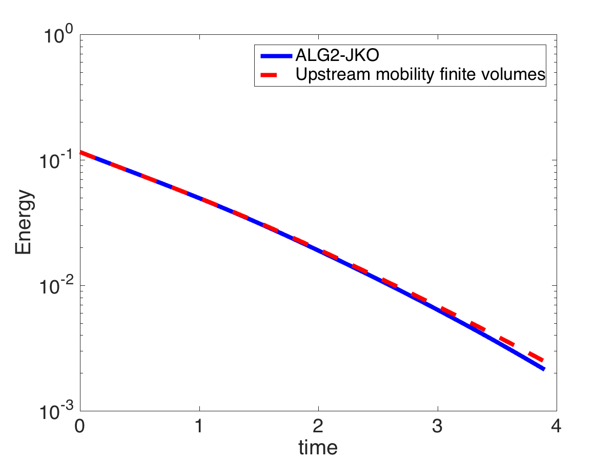
Then one computes for both scheme the relative energy , that we plot as a function of time on Figure 8. The convergence towards the equilibrium appears to be exponential in both cases.
4. Conclusion
We proposed to apply the ALG2-JKO scheme of [6] to simulate multiphase porous media flows. The results have been compared to the widely used upstream mobility finite volume scheme. The ALG2-JKO scheme appears to be robust w.r.t. the capillary pressure function and overall w.r.t. the viscosity ratios. The method is parameter free (the only parameter has a rather low influence and is chosen equal to 1 in the computations) and is unconditionally converging whatever the time step. This is a great advantage when compared to the Newton method that may require very small time steps in presence of large viscosity ratios. Moreover, the ALG2-JKO scheme preserves the positivity of the saturations, the constraint on the sum of the saturations, and it is locally conservative. Its main drawback concerns the restriction to linear mobility function so that formulas (15)–(16) hold (this can probably be extended to the non-physical case of concave mobilities [17] but we did not push into this direction). Finally, let us stress that the code depends only at stage (22) of the energy. Therefore, the extension of the ALG2-JKO approach to multiphase models with different energies (like for instance degenerate Cahn-Hilliard models [32, 12]) is not demanding once the code is written. A natural extension to this work would be to add source terms corresponding for instance to production wells. This would for instance require to adapt the material of [23] to our context.
Acknowledgements
CC was supported by the French National Research Agency (ANR) through grant ANR-13-JS01-0007-01 (project GEOPOR) and ANR-11-LABX0007-01 (Labex CEMPI). LM was partially supported by the Portuguese Science Fundation through FCT grant PTDC/MAT-STA/0975/2014. TOG was partially supported by the Fonds de la Recherche Scientifique - FNRS under Grant MIS F.4539.16.
References
- [1] A. Ait Hammou Oulhaj. Numerical analysis of a finite volume scheme for a seawater intrusion model with cross-diffusion in an unconfined aquifer. Numer. Methods Partial Differential Equations, 34(3):857-880, 2018.
- [2] Luigi Ambrosio, Nicola Gigli, and Giuseppe Savaré. Gradient flows: in metric spaces and in the space of probability measures. Springer Science & Business Media, 2008.
- [3] J. Bear and Y. Bachmat. Introduction to modeling of transport phenomena in porous media. Kluwer Academic Publishers, Dordrecht, The Netherlands, 1990.
- [4] J.-D. Benamou and Y. Brenier. A computational fluid mechanics solution to the Monge-Kantorovich mass transfer problem. Numer. Math., 84(3):375–393, 2000.
- [5] J.-D. Benamou, Y. Brenier, and K. Guittet. Numerical analysis of a multi-phasic mass transport problem. In Recent advances in the theory and applications of mass transport, volume 353 of Contemp. Math., pages 1–17. Amer. Math. Soc., Providence, RI, 2004.
- [6] J.-D. Benamou, G. Carlier, and M. Laborde. An augmented Lagrangian approach to Wasserstein gradient flows and applications. In Gradient flows: from theory to application, volume 54 of ESAIM Proc. Surveys, pages 1–17. EDP Sci., Les Ulis, 2016.
- [7] Y. Brenier and J. Jaffré. Upstream differencing for multiphase flow in reservoir simulation. SIAM J. Numer. Anal., 28(3):685–696, 1991.
- [8] Y. Brenier and M. Puel. Optimal multiphase transportation with prescribed momentum. ESAIM Control Optim. Calc. Var., 8:287–343 (electronic), 2002.
- [9] C. Cancès. Energy stable numerical methods for porous media flow type problems. HAL: hal-01719502, February 2018.
- [10] C. Cancès, T. O. Gallouët, and L. Monsaingeon. The gradient flow structure of immiscible incompressible two-phase flows in porous media. C. R. Acad. Sci. Paris Sér. I Math., 353:985–989, 2015.
- [11] C. Cancès, T. O. Gallouët, and L. Monsaingeon. Incompressible immiscible multiphase flows in porous media: a variational approach. Anal. PDE, 10(8):1845–1876, 2017.
- [12] C. Cancès, D. Matthes, and F. Nabet. A two-phase two-fluxes degenerate Cahn-Hilliard model as constrained Wasserstein gradient flow. HAL: hal-01665338, December 2017.
- [13] C. Cancès and F. Nabet. Finite volume approximation of a degenerate immiscible two-phase flow model of Cahn–Hilliard type. In C. Cancès and P. Omnes, editors, Finite Volumes for Complex Applications VIII - Methods and Theoretical Aspects : FVCA 8, Lille, France, June 2017, number 199 in Proceedings in Mathematics and Statistics, pages 431–438, Cham, 2017. Springer International Publishing.
- [14] H. Darcy. Les fontaines publiques de la ville de Dijon. Dalmont, Paris, 1856.
- [15] E. De Giorgi. New problems on minimizing movements. In Boundary value problems for partial differential equations and applications, volume 29 of RMA Res. Notes Appl. Math., pages 81–98. Masson, Paris, 1993.
- [16] K. Deimling. Nonlinear functional analysis. Springer-Verlag, Berlin, 1985.
- [17] J. Dolbeault, B. Nazaret, and G. Savaré. A new class of transport distances between measures. Calc. Var. Partial Differential Equations, 34(2):193–231, 2009.
- [18] J. Droniou, R. Eymard, T. Gallouët, C. Guichard, and R. Herbin. The gradient discretisation method . A framework for the discretisation and numerical analysis of linear and non-linear elliptic and parabolic problems, November 2016.
- [19] M. Erbar, K. Kuwada, and K.-T. Sturm. On the equivalence of the entropic curvature-dimension condition and Bochner’s inequality on metric measure spaces. Invent. Math., 201(3):993–1071, 2015.
- [20] R. Eymard, T. Gallouët, and R. Herbin. Finite volume methods. Ciarlet, P. G. (ed.) et al., in Handbook of numerical analysis. North-Holland, Amsterdam, pp. 713–1020, 2000.
- [21] R. Eymard, R. Herbin, and A. Michel. Mathematical study of a petroleum-engineering scheme. M2AN Math. Model. Numer. Anal., 37(6):937–972, 2003.
- [22] Michel Fortin and Roland Glowinski. Augmented Lagrangian methods, volume 15 of Studies in Mathematics and its Applications. North-Holland Publishing Co., Amsterdam, 1983. Applications to the numerical solution of boundary value problems, Translated from the French by B. Hunt and D. C. Spicer.
- [23] T. Gallouët, M. Laborde, and L. Monsaingeon. An unbalanced Optimal Transport splitting scheme for general advection-reaction-diffusion problems. HAL: hal-01508911, 2017.
- [24] F. Hecht. New development in FreeFEM++. J. Numer. Math., 20(3-4):251–265, 2012.
- [25] R. Jordan, D. Kinderlehrer, and F. Otto. The variational formulation of the Fokker-Planck equation. SIAM J. Math. Anal., 29(1):1–17, 1998.
- [26] G. Legendre and G. Turinici. Second-order in time schemes for gradient flows in Wasserstein and geodesic metric spaces. C. R. Acad. Sci. Paris Sér. I Math., 353(3):345-353, 2017.
- [27] S. Lisini. Nonlinear diffusion equations with variable coefficients as gradient flows in Wasserstein spaces. ESAIM Control Optim. Calc. Var., 15(3):712–740, 2009.
- [28] Christian Loeschcke. On the relaxation of a variational principle for the motion of a vortex sheet in perfect fluid. PhD thesis, Univ. Bonn, 2012.
- [29] D. Matthes, R. J. McCann, and G. Savaré. A family of nonlinear fourth order equations of gradient flow type. Comm. Partial Differential Equations, 34(11):1352–1397, 2009.
- [30] D. Matthes and S. Plazotta. A Variational Formulation of the BDF2 Method for Metric Gradient Flows. arXiv:1711.02935, 2017.
- [31] R. J. McCann. A convexity principle for interacting gases. Adv. Math., 128(1):153–179, 1997.
- [32] F. Otto and W. E. Thermodynamically driven incompressible fluid mixtures. J. Chem. Phys., 107(23):10177–10184, 1997.
- [33] N. Papadakis, G. Peyré, and E. Oudet. Optimal transport with proximal splitting. SIAM J. Imaging Sci., 7(1):212–238, 2014.
- [34] D. W Peaceman. Fundamentals of numerical reservoir simulation, volume 6 of Developments in Petroleum Science. Elsevier, 1977.
- [35] F. Santambrogio. Optimal Transport for Applied Mathematicians: Calculus of Variations, PDEs, and Modeling. Progress in Nonlinear Differential Equations and Their Applications 87. Birkhäuser Basel, 1 edition, 2015.
- [36] F. Santambrogio. Euclidean, metric, and Wasserstein gradient flows: an overview. Bulletin of Mathematical Sciences, 7(1):87–154, 2017.
- [37] C. Villani. Optimal transport, volume 338 of Grundlehren der Mathematischen Wissenschaften [Fundamental Principles of Mathematical Sciences]. Springer-Verlag, Berlin, 2009. Old and new.