Testing to distinguish measures on metric spaces
Abstract.
We study the problem of distinguishing between two distributions on a metric space; i.e., given metric measure spaces and , we are interested in the problem of determining from finite data whether or not is . The key is to use pairwise distances between observations and, employing a reconstruction theorem of Gromov, we can perform such a test using a two sample Kolmogorov–Smirnov test. A real analysis using phylogenetic trees and flu data is presented.
Keywords: Energy test; Fréchet mean; Kolmogorov–Smirnov two sample test; Reconstruction theorem.
1. Introduction
Statistical inference relies on the notion of observations coming from some random mechanism taking the form of a probability model. In some instances the formulation of such a probability model is difficult and an illustration of this occurs when observations arise in the form of phylogenetic trees. To undertake statistical inference here one would need a probability model on the space of trees with, say, leaves, and denoted by . However, before one can contemplate how to proceed statistically it is necessary to determine a metric on this space. A distance does exist which can be adequately used for statistical inference and this will be discussed later. For now we refer the reader to [1], [2] and [11] for background on statistical inference for phylogenetic trees.
Much of statistical inference takes place in Euclidean spaces; utilizing distances between parameters in , for example. In such metric spaces many useful concepts such as centroids and limit theorems exist. However, in other metric spaces, this is not necessarily the case and in such circumstances statistical inference becomes challenging. The particular task the present paper is concerned with is two sample hypothesis testing. That is, given two sets of randomly generated trees we wish to test that the two random generating mechanisms are the same. This is different from the hypothesis test considered in [12], who tested whether a true phylogenetic tree, regarded as an unknown parameter, is included in a specified set of trees or not. However, the theory we present goes beyond this specific space of trees and applies to more general metric spaces.
One such space, which we discuss only as a reference to provide illustration, arises in nonparametric density estimation problems. One uses distances, or divergences, between density or distributon functions; such as the distance and Kullback–Leibler divergence for the former, and any distance metricizing weak convergence of distribution functions, for the latter. Though an atypical problem in statistics, one could ask whether two sets of randomly generated distribution functions, , and , share the same generating mechanism; i.e. to test . For a nonparametric test one is going to struggle to find a framework in which to conduct such a test.
A parametric test could, for example, use the Dirichlet process ([7]) as a foundation. The Dirichlet process measure for is fully specified by a scale parameter and a centering distribution for which
In this case we would look only to check whether the mean and variance of matched those of for each . This would be however quite restrictive and miss other dissimilarities.
In order to undertake a nonparametric test we can utilize a metric metricizing weak convergence of distribution functions, such as the Prokhorov distance. From the observed sets of distribution functions we would compute the pairwise distances
These values from each set of distribution functions can then be used to construct a test. Indeed, [10] has shown that if is the matrix with entries then the distribution of characterizes, up to an isometry, the probability measure generating the . The isometry, say , would be such that . This basic idea, which we adapt, can be used to perform a two sample test for ; though the caveat is that the power for testing , which generates , against , which generates , will be no greater than the Type I error. However, we would not see this as a problem since the isometry alternatve is quite specific and unlikely to be present in practice; i.e. that is a specific deterministic transform of .
The space we are primarily concerned with is the space of phylogenetic trees with leaves; a non–Euclidean metric space. The celebrated work of [3] constructs a metric space on . The distance between two trees each with leaves is described in [3], and we refer the reader to this article for the details.
While this space has a rich geometric structure, it is far from Euclidean. Performing statistical inference in such non–Euclidean metric spaces is a problem of basic interest. In this paper, we focus on the problem of determining tests to distinguish finite samples and drawn from different measures and on a metric space . We will assume that and are Borel measures, is a Polish space, and is finite with respect to and , indeed . We approach the problem using the intrinsic structure of the metric measure spaces and following the geometric view introduced by Gromov, [10]. Gromov’s “mm-reconstruction theorem” shows that a metric measure space is characterized up to isomorphism by the induced distributions, via pushforward, under the “distance matrix” maps
where denotes the set of positive symmetric matrices and the map takes a set of points to the matrix such that .
Given two finite subsets , we use distance matrix distributions to specify and describe a non–parametric test for the hypothesis that and were drawn from identical measures, up to an isometry, on . We validate our test using synthetic data, and also comparing with an alternative test, as well as using the test on antigenic flu data; coming from the National Centre for Biotechnology Information (NCBI).
The technique we use is based on that of Gromov. We obtain a modification of his result by characterizing a probability measure by the distribution of the stochastic process
With data points we can partially observe such processes and this will form the basis of the test.
An array of tests which could be employed are based on the so–called Energy Statistics; see [16]. The energy distance between and is defined as
where is an independent copy of and an independent copy of . Tests for are therefore based on a sample estimate of given by
This is using a fundamentally different strategy from the one we use.
There are at least three identified problems with using tests based on . The first is that must be a Hilbert space (see [13]) in order for the condition , which is obviously essential. Secondly, it has recently been shown that such tests do not have the sufficient power they were originally thought to have; see [15]. Finally, the two sample test requires boostrap and permutation techniques in order to implement; see Section 6 in [16].
Another idea is to introduce a reference set and to consider a test based on the values and for all . See, for example, [5], though the authors are primarily proposing a test on a high dimensional Euclidean space. Our problem in the context of topological data would be how to choose in a meaningful way.
In section 2 we describe some theory which complements that of Gromov and provides the basis for the test statistic. In Section 3 we illuminate the theory of Section 2 by showing how things look in a particular setting where we can identify objects quite easily. Section 4 presents ilustrations including some real data analysis and section 5 concludes with a brief discussion.
2. Theory
We adapt the basic technique of Gromov. Note that Gromov’s results characterize the metric measure space only up to isomorphism; i.e., measure–preserving isometry. In our setting, this minor indeterminacy manifests itself via the fact that in order to test for to be characterized by , we must ensure the values of characterize the measure ; hence we assume that there does not exist a measure-preserving isometry . For suppose there exists such a for which
| (2.1) |
for all and . Then based on values of , we cannot infer .
Since this hypothesis is unknowable in practice, we will view our proposed test as testing for the hypothesis that the samples are drawn from measures on which coincide after application of some such , notably including possibly the identity map.
Define and is the mass assigned to the set . Then we define the valued stochastic process , indexed by , as
Hence, for example,
Theorem 2.1.
The joint distribution of with the being i.i.d. from characterize the process .
Proof. The moments
where , characterises the joint distribution of
for any choice of under the measure . It is seen that this is characterized by the joint distribution of
So this joint distribution characterizes the process through the finite dimensional distributions, which clearly satisfy the Kolmogorov consistency condition, thus completing the proof. ∎
Hence, if for measures and , i.e.
with and being i.i.d. from and , respectively, then
That is, the two processes share the same distribution.
Theorem 2.2.
Suppose the two processes and are equal in distribution and form a set of distinct paths. Also assume that and are distributions with densities and , respectively. That is, for .
for some measure . If there is no non–trivial bijection such that
for all and , then for all metric balls .
Proof. For ease of exposition we first assume that is a discrete measure and that is the mass assigned to for measure . Assume that in that there exist some metric ball such that . Given that form a set of distinct paths in for each , and similarly for , there exists a non–trivial bijection such that for all and all , and . These statements follow from the assumption .
Therefore, from the former of these statements we have
and the right side can be written as
| (2.2) |
by a simple transformation. Now using the latter of the statements, (2.2) is given by
and hence for all , contradicting the assumption in the statement of the theorem; hence, for all metric balls , .
The argument for other measures follows similarly. For now we have the two results and that if then . Hence, from the former result we obtain
and from the latter that
where denotes the usual indicator function. ∎
There is no asymmetry here in the use of in the statement of the thereom; for if no exists for and , then no exists for either.
We now show that the conclusion of Theorem 2.2 implies . The argument we give is standard; e.g., see [4] for a more comprehensive discussion. Throughout, we work with a fixed metric space . Let denote a collection of subsets of . For a given Borel measure on we define an outer measure on by the formula
Here we are considering only countable covers of .
Let denote the collection of metric balls in of radius . We define a metric outer measure by the formula
Note that for , . Associated to a metric outer measure is a Borel measure; we will abusively denote this by as well.
Now, the hypothesis we are working with is that we have two measures on , and , such that for any metric ball we have the equality . Therefore, the metric outer measures and associated Borel measures and coincide.
We would like to specify conditions under which the original measures and must coincide. We will do this by providing conditions under which and ; that is, conditions under which a measure is determined by its values on metric balls.
Lemma 2.1.
For any metric measure space and subset , we have
Proof. This follows from the fact that for any fixed we can approximate arbitrarily closely by taking a cover of by metric balls. ∎
In order to show that , we need a hypothesis on . All of the relevant hypotheses amount to control on the approximation of an arbitrary set by metric balls, as one would expect. Here is a fairly common hypothesis that suffices: Recall that a measure is doubling if there exists a finite constant such that for all and . We need the following standard result about doubling measures.
Proposition 2.1.
Let be a metric measure space with a doubling measure. For any open , there exists a countable collection of pairwise disjoint balls such that and .
We can now prove that when is a metric measure space with a doubling measure, for all . It suffices to consider open. Furthermore, it is clear that and are also doubling measures if is, and so for we apply the proposition to and conclude that
The desired inequality now follows by letting go to zero.
3. Theory on space of normal density functions
In this section we provide an illustration of the theory in Section 2 so as to expose some of the key points in perhaps more familiar statistical territory. Though we need point out statistical testing in the environment of normal density functions to be described would not be done this way; we use it merely to illuminate Section 2. We let be the non–Euclidean space of normal density functions and is the Hellinger distance. So and
For further simplicity, let us assume the normal densities both have mean , so
A distance preserving bijective isometry exists here; it is , and it is easy to see that . Hence, our test in this case would not be able to distinguish between the densities and . To elaborate, from we would have distances and, for example, the distances from would be so we would conclude they were from the same source. However, we would not see this as a problem, given the very specific nature of the and .
To consider the stochastic process , let us consider , with . This becomes
where . Hence
If, for example, is standard exponential, then
and is the random path as a function of from 0 to 1, and with the chosen from . Here we see, for example, that for different , the paths are different.
However, we note in this case that does not characterize due to the isometry.
To motivate the test described in the paper we would be testing where we observe and for , with and . If we knew that the Fréchet means were both, say , with known, then we would compare the samples
and use a Kolmogorov–Smirnov two sample test. This makes sense because
is equivalent to
This implies that
where
which implies . This does not hold, for we can have , when . That is, under this special existence of the known Fréchet mean, the appearance of the isometry arises when only.
Note here that the Fréchet mean is given by the which minimizes
If a Fréchet mean does exist and is unique for each sample, but is unknown, then it can be estimated from the data. Indeed, we estimate the mean from the sample as which minimizes, over ,
A similar strategy is used to get the Fréchet mean for the sample. The validity of a Kolmogorov–Smirnov test with a reduced degree of freedom, and with samples,
is now provided by the theory in Section 2. The reasoning is that up to an isometry, the rows from ; i.e. all characterize asymptotically. We use the minimum sum row in order to replicate as close as possible the case with the known Fréchet mean.
The samples being compared are
The first set yields an empirical distribution, say , and the second set an empirical distribution, say . We then test for using the two sample Kolmogorov–Smirnov test.
Aside from the isometry, , if these two samples pass the two sample Kolmogorov–Smirnov test with samples, then we do not reject the hypothesis .
4. Test and Illustrations
Suppose we have two samples and from and , respectively. Now if and are identical, then for each and , the distributions of
are also identical. Moreover, from the theory in Section 2, we have that if the asymptotic sequences share the same distribution then and are the same. Hence, our proposed test is to select the two sets of values using carefully chosen and and to then perform a two sample Kolmogorov–Smirnov test; see for example [6]. Our choices for and are
respectively. This ensures we are comparing like rows from each matrix and and moreover the choice and can be seen as a best representative of a location for the measures in that they are similar to Fréchet means. More on this in the discussion in Section 5.
4.1. Comparison with synthetic data
To compare our test with another, we use a test statistic from the distance based test given in [16], and known as the energy test. The test statistic is given by
This is currently a popular choice for comparing two data sets. However, there is a problem in that the critical value will depend on the distributions of and and hence a bootstrap procedure is required in order to complete the test.
To implement the two sample energy test we use bootstrap methods; since the distribution of the null hypothesis that and come from the same source actually depends on that source. Hence, to get a critical value we compute , which is obtained by randomly splitting the vector into two equally sized sets and computing the energy statistic based on such a partition. The 95% quantile value from the , for a large , serves as the critical value, written as . We then compute and reject the hypothesis for and coming from the same source if .
We compare this with the conditional Kolmogorov–Smirnov test. Hence, we use the test statistic
where is the empirical distribution of the and the corresponding empirical distribution function of the Here we reject the null hypothesis at the 95% level of significance if , in keeping with the Kolmogorov–Smirnov two–sample test theory.
| -test power | –test power | |
|---|---|---|
| 1.2 | 0.06 | 0.06 |
| 1.4 | 0.20 | 0.15 |
| 1.6 | 0.42 | 0.33 |
| 1.8 | 0.61 | 0.43 |
| 2.0 | 0.81 | 0.70 |
| 2.2 | 0.90 | 0.84 |
| 2.4 | 0.95 | 0.92 |
To undertake an initial simulation study we take the as independent and identically distributed from the standard normal distribution and take the as independent normal with mean 0 and variance . We then, in the case of the energy test, compute the power of the test for a range of and the results are reported in Table 1.
To complete the settings for the comparison, we took and the number of simulations to record the power value was based on a Monte Carlo sample size of 1000. The sample size was . The distance employed is the absolute value between and . While the observations are simple it is the distribution of which matters and even if the are generated according to some highly complex and high–dimensional setting, the distribution of the may yet be not unusual.
4.2. Real data analysis
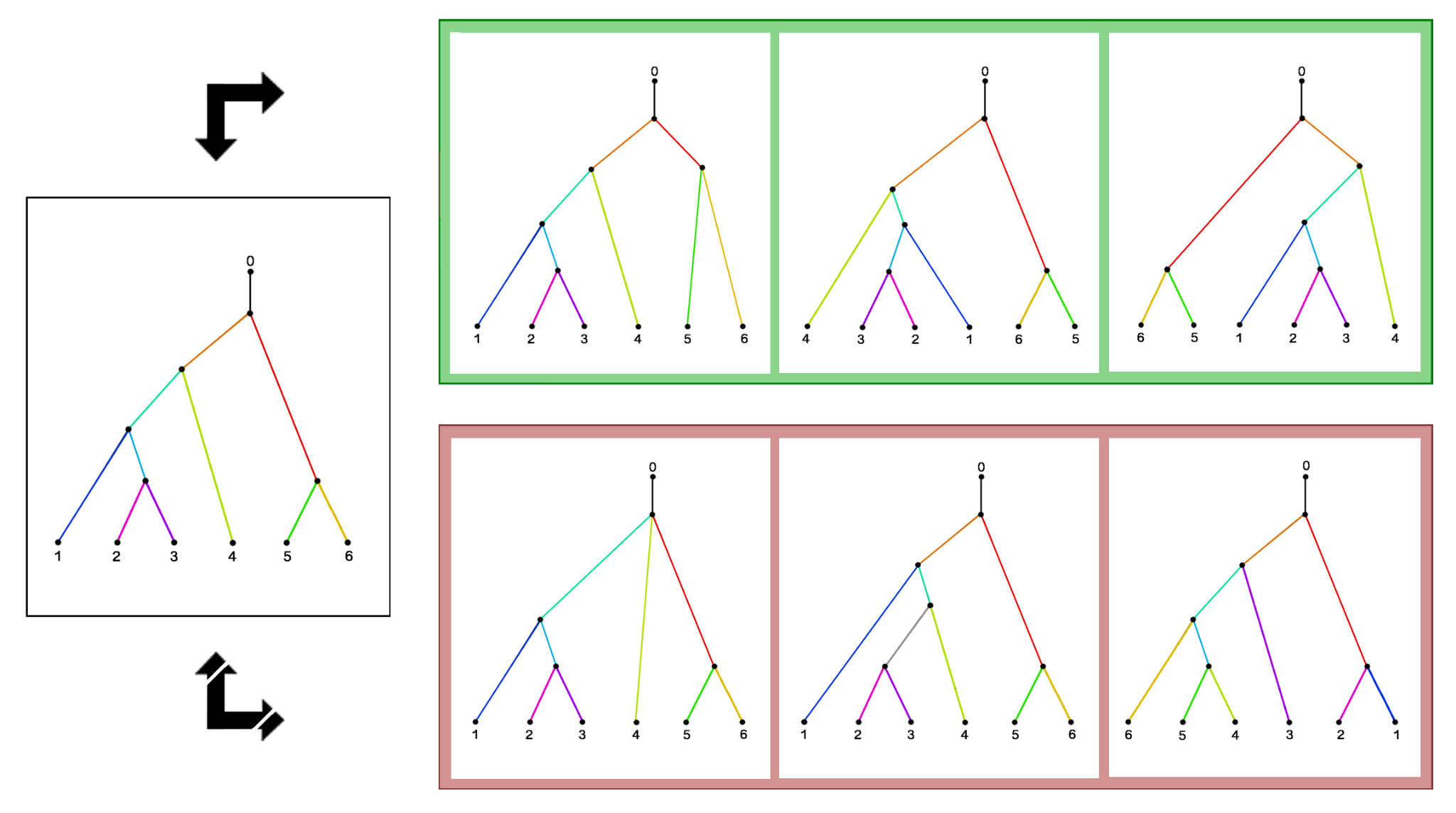
A real data analysis is now presented. In the paper [18], the authors used hemagglutinin, an antigenic surface glycoprotein, coding sequences in RNA from flu samples collected in the United States between 1993 and 2016. These samples were originally obtained from the GI–SAID EpiFlu database and then processed. Small phylogenetic trees with three, four, and five leaves were constructed from randomly drawn sequential samples; i.e., representing samples from three, four, or five consecutive years, the result was empirical distributions in the BHV metric space of phylogenetic trees; see [3]. A phylogenetic tree in is an acyclic connected graph with a distinguished vertex (the root) and vertices of degree , the leaves, along with labels in for the leaves and weights in for the edges that are not incident to a leaf. For a given tree topology, a tree is then completely specified by a vector in with all coordinates non–negative. An illustration of a tree with 3 leaves is given in Fig 1.
Note that switching labels 2 and 3 results in the same tree; we do not take account of the embedding of the tree in the plane. More general illustrations of trees with the same and distinct topologies are given in Fig 2.
To form the metric space , we glue together these Euclidean orthants labelled by tree topologies so that two orthants are adjacent if the two topologies coincide after collapsing a single edge to in each one. Such a transformation is often referred to as a tree rotation.

The metric is now computed as the minimal piecewise linear path between trees; see Fig 3 for an example of a path across orthants in tree space. Note however that many paths go through the “cone point”, which is the tree with all internal edges of length . As another illustration of the distance, consider the tree from Fig 1 and the tree obtained by switching 1 and 2 (which is a distinct tree). To compute the distance we move the node for 2 and 3 in Fig 1 to the root by collapsing the edge between it and the root, so that now all the leaves hang from the same point, and then rearrange the leaves appropriately. The distance needed to move the nodes to the root and then out again constitutes the overall distance. In more complicated trees, the distance is harder to visualize; nonetheless, there are (polynomial-time) computer algorithms to compute it [14].
In order to interpret the results of our test, we need to understand the isometries of the space of phylogenetic trees. In [9], it is shown that the only isometries are given by permuting labels; a permutation on the labels for the leaves might transform the topology of a tree but clearly preserves distances between trees. As before, we do not see this as a problem as we would not anticipate the two generating mechanisms for the two sets of trees to be separated by such a permutation.


The purpose of looking at these distributions in the BHV metric spaces was to use the metric to compare distributions for different seasons; reliable ways to do this would lead to predictions about vaccine design and effectiveness. In [18], a crude test statistic involving the distance to the centroid turned out to be surprisingly effective for predicting vaccine efficacy. As a representative experiment to validate our distribution test, we compared empirical distributions computed from windows centered around the 1996 and the 2007 seasons, using data supplied by the authors of [18]. The metric distance was computed using software implementing the fast algorithm of [14]. We used 1000 samples from each distribution.
Both tests; i.e. the and tests rejected, at a 95% level of significance, the null hypothesis that the two distributions generating and are the same. The Kolmogorov–Smirnov test is remarkably quick to implement. However, for the two sample energy test there is an extremely time consuming computation of the critical value. To confirm the distribution of the distances are regular looking, we plot the distribution functions of and , with and chosen as described previously. The two together are shown in Fig 4.
Given the large number of data, we split the data matrix for the , the 1996 flu data, into two independent blocks forming data matrix based on real data and data matrix based on real data . We now perform the Kolmogorov–Smirnov test for these two matrices and in this case we accept the null hypothesis. We illustrate the two distribution functions in Fig 5.
5. Discussion
Hypothesis testing in the context of topological, non–Euclidean, data poses unique challenges. Even the problem of testing whether two sets of data have the same source is difficult. Our solution to this is based on theory presented by Gromov which allows us to use the Kolmogorov–Smirnov test on two carefully chosen sets of distances; being those from the minimum row sums of the reconstruction matrix.
On the other hand, an alternative test based on the energy distance is also possible. Problems with this are that in the two–sample test one has to compute the critical value using permutations and with large data sets this procedure can become prohibitively time consuming.
We have demonstrated that our test is substantially faster and moreover when there is a simple scale difference between the two samples, it has superior power to that of the energy test.
For further insights into the test, assume that and have the same Fréchet mean ; then we can test for using samples and A suitable test would be the Kolmogorov–Smirnov test with points.
Ruling out any isometries, we can assume that Not knowing we would use the empirical samples and where minimizes over the sum and similarly for . This can also be tested using the Kolmogorov–Smirnov test with now a reduction to points. This is of course the test we use. The theory attributable to Gromov says this is also the test of choice when may not exist and the point of the use of empirical samples and replacing allows for the rejection of the hypothesis when the means, if they exist, are different.
Another interesting example also arises in the context of topological data analysis; the space of “barcodes”, which is the output of the determination of persistent homology (e.g., see [17, 8]) forms a metric space which is not Euclidean.
Finally we mention that there is no reason why we can not handle and sample sizes from each measure; we simply chose to illustrate the test when sample sizes are equal.
Acknowledgements
The first author was supported in part by AFOSR grant FA9550-15-1-0302 and NIH grants 5U54CA193313 and GG010211-R01-HIV, and the third author from NSF grants DMS 1506879 and 1612891. The first author would like to thank Raul Rabadan, Sakellarios Zairis, and Hossein Khiabanian for helpful conversations.
References
- [1] D. J. Aldous. Probability distributions on cladograms. In Random Discrete Structures; (D.J.Aldous and R.Pemantle, eds.) Springer–Verlag, Berlin, pages 1–18, 1996.
- [2] D. J. Aldous. Stochastic models and descriptive statistics for phylogenetic trees, from yule to today. Stat. Sci., 16:23–34, 2001.
- [3] L. J. Billera, S. P. Holmes, and K. Vogtmann. Geometry of the space of phylogenetic trees. Advances in Applied Mathematics, 27(4):733–767, 2001.
- [4] B. Buet and G. P. Leonardi. Recovering measures from approximate values on balls. Ann. Acad. Sci. Fenn. Math., 41:947–972, 2016.
- [5] X. Cheng, A. Cloninger, and R. R. Coifman. Two–sample statistics based on anisotropic kernels. Preprint, arXiv:1709.05006v2, 2017.
- [6] G. W. Corder and D. I. Foreman. Nonparametric Statistics: A Step–by–Step Approach. John Wiley & Sons, 2014.
- [7] T. S. Ferguson. A Bayesian analysis of some nonparametric problems. Ann. Statist., 1:209–230, 1973.
- [8] R. Ghrist. Barcodes: The persistent topology of data. Bulletin of the American Mathematical Society, 45(1):61–75, 2008.
- [9] G. Grindstaff. Isometries of the space of phylogenetic trees. preprint, 2018.
- [10] M. Gromov. Hyperbolic Groups. Springer, 1987.
- [11] S. Holmes. Statistics for phylogenetic trees. Theor. Pop. Biol., 63:17–32, 2003.
- [12] S. Holmes. Statistical approach to tests involving phylogenies. In In Mathematics of Evolution and Phylogeny; (O. Gascuel, ed.) Oxford University Press, U.S.A., 2007.
- [13] R. Lyons. Distance covariance in metric spaces. Ann. Probab., 41(5):3284–3305, 2013.
- [14] M. Owen and J. S. Provan. A fast algorithm for computing geodesic distances in tree space. IEEE/ACM Transactions on Computational Biology and Bioinformatics, 8:2–13, 2011.
- [15] A. Ramdas, S. J. Reddi, B. Póczos, A. Singh, and L. Wasserman. On the decreasing power of kernel and distance based nonparametric hypothesis tests in high dimensions. In Twenty-Ninth AAAI Conference on Artificial Intelligence, 2015.
- [16] G. J. Székely and M. L. Rizzo. Energy statistics: A class of statistics based on distances. Journal of Statistical Planning and Inference, 143(8):1249–1272, 2013.
- [17] S. Weinberger. What is … persistent homology? Notices AMS, 58(01):36–39, 2011.
- [18] S. Zairis, H. Khiabanian, A.J. Blumberg, and R. Rabadan. Genomic data analysis in tree spaces. Preprint, arXiv:1607.07503, 2016.