Secure Range Queries for Multiple Users
Abstract
Order-preserving encryption allows encrypting data, while still enabling efficient range queries on the encrypted data. Moreover, it does not require any change to the database management system, because comparison operates on ciphertexts as on plaintexts. This makes order-preserving encryption schemes very suitable for data outsourcing in cloud computing scenarios. However, all order-preserving encryption schemes are necessarily symmetric limiting the use case to one client and one server. Imagine a scenario where a Data Owner encrypts its data before outsourcing it to the Cloud Service Provider and a Data Analyst wants to execute private range queries on this data. This scenario occurs in many cases of collaborative machine learning where data source and processor are different entities. Then either the Data Owner must reveal its encryption key or the Data Analyst must reveal the private queries. In this paper, we overcome this limitation by allowing the equivalent of a public-key order-preserving encryption. We present a secure multiparty protocol that enables secure range queries for multiple users. In this scheme, the Data Analyst cooperates with the Data Owner and the Cloud Service Provider in order to order-preserving encrypt the private range queries without revealing any other information to the parties. The basic idea of our scheme is to replace encryption with a secure, interactive protocol. In this protocol, we combine order-preserving encryption based on binary search trees with homomorphic encryption and garbled circuits achieving security against passive adversaries with sublinear communication and computation complexity. We apply our construction to different order-preserving encryption schemes including frequency-hiding order-preserving encryption which can withstand many of the popularized attacks on order-preserving encryption. We implemented our scheme and observed that if the database size of the Data Owner has 1 million entries it takes only about 0.3 s on average via a loopback interface (1.3 s via a LAN) to encrypt an input of the Data Analyst.
I Introduction
In cloud computing, companies use a network of remote servers hosted by a service provider on the Internet to store, manage, and process data, rather than a local server or a personal computer. Naively this would imply that Data Owners must give up either the security of the data or the functionality of processing the data. Therefore companies are reluctant to migrate their sensitive data to the cloud. However, different techniques, such as secure multiparty computation [38, 24, 16, 33, 27, 8], homomorphic encryption [15, 31, 9] or order-preserving encryption [1, 5, 6, 35, 34, 20, 19], exist that enable cloud users to encrypt their data before outsourcing it to the cloud while still be able to process and search on the outsourced and encrypted data without decrypting it. Order-preserving encryption (OPE) allows encrypting data, while still enabling efficient range queries on the encrypted data. Moreover it does not require any change to the database management system, because comparison operates on ciphertexts. This makes order-preserving encryption schemes very suitable for data outsourcing in cloud computing scenarios, since it can be retrofitted to existing applications.
However, all OPE schemes are necessarily symmetric limiting the use case to one client and one server. This is due to the fact that a public-key encryption would allow a binary search on the ciphertext. Imagine a scenario where a Data Owner (DO) encrypts its data before outsourcing it to the Cloud Service Provider (CSP) and a Data Analyst (DA) wants to execute private range queries on this data. Then either the Data Owner must reveal its encryption key, since order-preserving encryption is symmetric, or the Data Analyst must reveal the private queries.
This distinction between DO and DA occurs in many cases of collaborative data analysis, data mining and machine learning. In such scenarios, multiple parties need to jointly conduct data analysis tasks based on their private inputs. As concrete examples from the literature consider, e.g., supply chain management, collaborative forecasting, benchmarking, criminal investigation, smart metering, etc.) [11, 3, 2, 18]. Although in these scenarios plaintext information sharing would be a viable alternative, participants are reluctant to share their information with others. This reluctance is quite rational and commonly observed in practice. It is due to the fact that the implications of the information are unknown or hard to assess. For example, sharing the information could weaken their negotiation position, impact customers’ market information by revealing corporate performance and strategies or impact reputation [3, 2, 7].
In this paper, we overcome the limitation of private range querying on order-preserving encrypted data by allowing the equivalent of a public-key encryption. Our idea is to replace public-key encryption with a secure, interactive protocol. Non-interactive binary search on the ciphertext is no longer feasible, since every encryption requires the participation of the Data Owner who can rate limit (i.e., control the rate of query sent by) the Data Analyst.
Since neither the DA wants to reveal his query value nor the DO his encryption state (key), this is clearly an instance of a secure computation where two or more parties compute on their secret inputs without revealing anything but the result. In an ideal world the DA and DO would perform a two-party secure computation for the encryption of the query value and then the DA would send the encrypted value as part of an SQL query to the CSP. However, this two-party secure computation is necessarily linear in the encryption state (key) and hence the size of the database. Our key insight of this paper is that we can construct an encryption with logarithmic complexity in the size of the database by involving the CSP in a three-party secure computation without sacrificing any security, since the CSP will learn the encrypted query value in any case. One may conjecture that in this construction the encryption key of the DO may be outsourced to secure hardware in the CSP simplifying the protocol to two parties, but that would prevent the DO from rate limiting the encryption and the binary search attack would be a threat again, even if the protocol were otherwise secure.
We call our protocol oblivious order-preserving encryption. We implemented it and an encryption by the DA takes 0.3 seconds using the loopback interface and 1.3 seconds using a LAN in a large data center.
Our contributions are as follows:
- •
First, we introduce a novel notion of oblivious order-preserving encryption. This scheme allows a DA to execute private range queries on an order-preserving encrypted database.
- •
- •
- •
Finally, we implement and evaluate our scheme.
The remainder of the paper is structured as follows. We review related work in Section II and preliminaries in Section III before defining correctness and security of oblivious OPE in Section IV. Section V describes our scheme for the case where the underlying OPE scheme is deterministic and prove its correctness and security. In Section VI we discuss integer comparison and equality test with garbled circuit and how we use it in our schemes. The non-deterministic case is handled in Section VII. We discuss implementations details and evaluation in Section VIII before concluding our work in Section IX.
II Related Work
Order-preserving encryption can be classified into stateless schemes (see Section II-A) and stateful schemes (see Section II-B). Our work is concerned with stateful schemes and hence we introduce some of their algorithms in this section. However, we review stateless schemes and their security definitions first in order to distinguish them from stateful schemes.
II-A Stateless Order-preserving Encryption
Order-preserving encryption ensures that the order relation of the ciphertexts is the same as the order of the corresponding plaintexts. This allows to efficiently search on the ciphertexts using binary search or perform range queries without decrypting the ciphertexts. The concept of order-preserving encryption was introduced in the database community by Agrawal et al. [1]. The cryptographic study of Agrawal et al.’s scheme was first initiated by [5], which proposed an ideal security definition IND-OCPA11 1 IND-OCPA means indistinguishability under ordered chosen plaintext attacks and requires that OPE schemes must reveal no additional information about the plaintext values besides their order for OPE. The authors proved that under certain implicit assumptions IND-OCPA is infeasible to achieve. Their proposed scheme was first implemented in the CryptDB tool of Popa et al. [35] and attacked by Naveed et al. [30]. In [6] Boldyreva et al. further improved the security and introduced modular order-preserving encryption (MOPE). MOPE adds a secret modular offset to each plaintext value before it is encrypted. It improves the security of OPE, as it does not leak any information about plaintext location, but still does not provide ideal IND-OCPA security. Moreover Mavroforakis et al. showed that executing range queries via MOPE in a naive way allows the adversary to learn the secret offset and so negating any potential security gains. They address this vulnerability by introducing query execution algorithms for MOPE [29]. However, this algorithm assumes a uniform distribution of data and has already been attacked in [12]. In a different strand of work Teranishi et al. improve the security of stateless order-preserving encryption by randomly introducing larger gaps in the ciphertexts [37]. However, they necessarily also fail at providing ideal security.
II-B Stateful Order-preserving Encryption
Popa et al. were the first to observe that one can avoid the impossibility result of [5] by giving up certain restrictions of OPE. As result of their observations they introduced mutable OPE [34]. Their first observation was that most OPE applications only require a less restrictive interface than that of encryption schemes. Their encryption scheme is therefore implemented as an interactive protocol running between a client that also owns the data to be encrypted and an honest-but-curious server that stores the data. Moreover, it is acceptable that a small number of ciphertexts of already-encrypted values change over time as new plaintexts are encrypted. With this relaxed definition their scheme was the first OPE scheme to achieve ideal security.
Popa et al.’s scheme (mOPE1) [34]. The basic idea of Popa et al.’s scheme is to have the encoded values organized at the server in a binary search tree (OPE-tree). Specifically the server stores the state of the encryption scheme in a table (OPE-table). The state contains ciphertexts consisting of a deterministic AES ciphertext and the order (OPE Encoding) of the corresponding plaintext. To encrypt a new value the server reconstructs the OPE-tree from the OPE-table and traverses it. In each step of the traversal the client receives the current node of the search tree, decrypts and compares it with . If is smaller (resp. larger) then the client recursively proceeds with the left (resp. right) child node of . An edge to the left (resp. to the right) is encoded as 0 (resp. 1). The OPE encoding of is then the path from the root of the tree to padded with to the same length . To ensure that the length of OPE encoding do not exceed the defined length , the server must occasionally perform balancing operations. This updates some order in the OPE table (i.e. the OPE encoding of some already encrypted values mutate to another encoding).
Kerschbaum and Schröpfer’s scheme (mOPE2) [20]. The insertion cost of Popa et al’s scheme is high, because the tree traversal must be interactive between the client and the server. To tackle this problem Kerschbaum and Schröpfer proposed in [20] another ideal secure, but significantly more efficient, OPE scheme. Both schemes use binary search and are mutable, but the main difference is that in the scheme of [20] the state is not stored on the server but on the client. Moreover the client chooses a range for the order. For each plaintext and the corresponding OPE encoding the client maintains a pair in the state. To insert a new plaintext the client finds two pairs , in the state such that and computes the OPE encoding as follows:
- •
if then the OPE encoding of is
- •
The encryption algorithm is keyless and the only secret information is the state which grows with the number of encryptions of distinct plaintexts. The client uses a dictionary to keep the state small and hence does not need to store a copy of the data.
Kerschbaum’s scheme (mOPE3) [19]. Deterministic OPE schemes [1, 5, 34, 20, 37] are vulnerable to many attacks like: frequency analysis, sorting attack, cumulative attack [30, 17]. To increase the security of OPE Kerschbaum first introduced in [19] a new security definition called indistinguishability under frequency-analyzing ordered chosen plaintext attack (IND-FAOCPA) that is strictly stronger than IND-OCPA. Second he proposed a novel OPE scheme mOPE3 that is secure under this new security definition. The basic idea of this scheme is to randomize ciphertexts such that no frequency information from repeated ciphertexts leaks. It borrows the ideas of [20] with a modification that re-encrypts the same plaintext with a different ciphertext. First client and server state are as by mOPE2. The order ranges from to as by mOPE2. The algorithm traverses the OPE-tree by going to the left or to the right depending on the comparison between the new plaintext and nodes of the tree. However, if the value being encrypted is equal to some value in the tree then the algorithm traverses the tree depending on the outcome of a random coin. Finally, if there is no more node to traverse the algorithm rebalances the tree if necessary and then computes the ciphertext similarly to .
In subsequent independent analysis [17] this encryption scheme has been shown to be significantly more secure to the attacks against order-preserving encryption (albeit not perfectly secure).
III Preliminaries
III-A Problem Statement
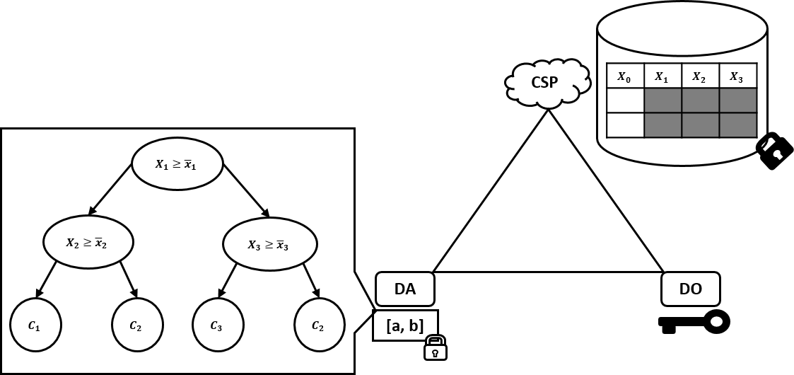
Our work is motivated by the following scenario. Assume a Data Owner encrypts its data with an order-preserving encryption, stores the encrypted data in a cloud database held by a Cloud Service Provider, and retains the encryption key. A Data Analyst wants to perform some analysis on the encrypted data. To this end it holds, e.g., a private machine learning model involving comparisons. In a supply chain scenario, the Data Analyst could be a supplier (manufacturer) wanting to optimize its manufacturing process based on data owned by its buyer (another supplier or distributor).
For instance, we assume the model to be a decision tree as pictured in Figure 1, where the are the thresholds and is the input vector (that maps to corresponding columns in the Data Owner’s database) to be classified. In order to use the model for classification the Data Analyst transforms the decision tree into range queries, e.g., for class we have the query . More precisely the Data Analyst wants to execute queries like in equations 1 and 2, where we assume to be public.
| (1) | |||
| (2) |
However, as the database is encrypted (i.e. columns , and are OPE encrypted) the Data Analyst needs ciphertexts of the thresholds . In [36], Taigel et. al. describes an approach that combines decision tree classification and OPE to enable privacy-preserving forecasting of maintenance demand based on distributed condition data. They consider the problem of a Maintenance, Repair, and Overhaul (MRO) provider from the aerospace industry that provides maintenance services to their customers’ (e.g., commercial airlines or air forces) jet engines. The customers as Data Owners consider the real condition data of their airliners as very sensitive and therefore this data is stored encrypted in a cloud database using OPE. The MRO provider as Data Analyst holds a decision tree that can predict the probability of maintenance, repair, and overhaul of spare parts. However, the classification of an individual spare part is not necessary, but only aggregated numbers such as returned by Equation 1. The aggregated numbers then allow the MRO to compute the forecast without violating the privacy of the real condition data. In [36], they provide privacy only for the customer, while we want to allow privacy for both customer and MRO provider.
Order-preserving encryption is necessarily symmetric, thus only the Data Owner can encrypt and decrypt the data stored on the cloud server. If the Data Analyst needs to obtain a ciphertext for a query, it can just send the plaintext threshold to the Data Owner. However, if the model contains intellectual property which the Data Analyst wants to remain protected, then this free sharing of information is no longer possible. Our goal is to allow the data analysis to be performed efficiently without revealing any sensitive information in the query and without revealing the key to the order-preserving encryption.
We now review a few building blocks used in our construction of oblivious order-preserving encryption.
III-B Secure Multiparty Computation
Secure multiparty computation (SMC) is a cryptographic technique that allows several parties to compute a function on their private inputs without revealing any information other than the function’s output. A classical example in the literature is the so called Yao’s millionaire’s problem introduced in [38]. Two millionaires are interested in knowing which of them is richer without revealing their actual wealth. Formally we have a set of parties , each with its own private input and they want to compute the function 33 3 The output of each party can also be private, in this case . without disclosing their private inputs.
Security of SMC protocols is often defined by comparison to an ideal model. In that model parties privately send their input to a trusted third party (TTP). Then the TTP computes the outcome of the function on their behalf, sends the corresponding result to each party and forgets about the private inputs. In the real model parties emulate the ideal model by executing a cryptographic protocol to perform the computation. At the end only the result should be revealed and nothing else. A SMC protocol is then said to be secure if the adversary can learn only the result of the computation and data that can be deduced from this result and known inputs [16, 8, 14].
An important issue to consider when defining the security of SMC is the adversary’s power. There exists many security models, but the semi-honest and the malicious adversary model are the most popular [16, 8]. In the semi-honest (a.k.a honest-but-curious) model parties behave passively and follow the protocol specification. However, the adversary can obtain the internal state of corrupted parties and uses this to learn more information. In contrast, a malicious adversary is active and instructs corrupted parties to deviate from the protocol specification.
III-C Yao’s Garbled Circuit
Yao’s initial protocol for secure two-party computation uses a technique called Garbled Circuits (GC). A GC can be used to execute a function over symmetrically encrypted inputs. In this section, we recall the idea of GC protocol and refer to [38, 26, 33, 27, 13, 4] for more technical description of circuit garbling and its implementation. Let be a function over two inputs and , then a garbling scheme consists of a five-tuple of algorithms . The original function is encoded as circuit that the function can evaluate. On input and security parameter , algorithm returns a triple of strings . The string describes a garbled function, , that maps each pair of garbled inputs to a garbled output . The string describes an encoding function, , that maps initial inputs to garbled inputs , . The String describes a decoding function, , that maps a garbled output to a final output . The garbling scheme is correct if [4].
A GC protocol is a 2-party protocol consisting of a generator (Gen) and an evaluator (Eva) with input and respectively. On input and , Gen runs and parses as . Then she sends and to Eva, where represents the -th bit of . Now the parties execute an oblivious transfer protocol with Eva having selection string and Gen having inputs (. As a result, Eva obtains and Gen learns nothing. Finally, Eva evaluates and outputs .
III-D Homomorphic Encryption
A homomorphic encryption scheme is an encryption scheme that allows computations on ciphertexts by generating an encrypted result whose decryption matches the result of operations on the corresponding plaintexts. With fully homomorphic encryption schemes [15] one can compute any efficiently computable function. However, with the current state of the art, their computational overhead is still too high for practical applications. Efficient alternatives are additive homomorphic encryption schemes, e.g.: Paillier [31, 9]. They allow specific arithmetic operations on plaintexts, by applying an efficient operation on the ciphertexts. Let denote the probabilistic encryption of a plaintext . Then the following addition property holds , i.e., by multiplying two ciphertexts one obtains a ciphertext of the sum. In our protocol we will use the public-key encryption scheme of Paillier [31].
III-E Overview of Our Construction
In theory generic SMC allows to compute any efficiently computable function. However, any generic SMC is at least linear in the input size, which in this case is the number of encrypted values in the database. The idea of our solution is to exploit the inherent, i.e. implied by input and output, leakage of Popa et. al.’s OPE scheme making our oblivious OPE sublinear in the database size. Furthermore, we exploit the advantage of (homomorphic) encryption allowing a unique, persistent OPE state stored at the CSP while being able to generate secure inputs for the SMC protocol and the advantage of garbled circuits allowing efficient, yet provably secure comparison. Our oblivious order-preserving encryption is therefore a mixed-technique, secure multi-party computation protocol between the Data Owner, the Data Analyst and the Cloud Service Provider in the semi-honest model.
In detail, our protocol proceeds as follows: The Data Owner outsources its OPE state to the cloud-service provider. As already described, the state consists of an OPE-table of ciphertext, order pairs. However, in oblivious order-preserving encryption the ciphertext is created using an additively homomorphic public-key encryption scheme instead of standard symmetric encryption. When the DA traverses the state in order to encrypt a query plaintext, the CSP creates secret shares44 4 Secret shares are random values that add up to the plaintext. using the homomorphic property. One secret share is sent to the DA and one to the DO. The DA and DO then engage in a secure two-party computation using Yao’s Garbled Circuits in order to compare the reconstruction of the secret shares (done in the garbled circuit) to the query plaintext of the DA. The result of this comparison is again secret shared between DA and DO, i.e., neither will know whether the query plaintext is above or below the current node in the traversal. Both parties – DA and DO – send their secret shares of the comparison result to the CSP which then can determine the next node in the traversal. These steps continue until the query plaintext has been sorted into the OPE-table and the CSP has an order-preserving encoding that can be sent to the DA. A significant complication arises from this order-preserving encoding, since it must not reveal the result of the comparison protocols to the DA (although it may be correlated to the results). In the next two sections we provide the detailed, step-by-step formalization of the construction.
IV Correctness and Security Definitions
In this section we first present the system architecture and then define correctness and security of oblivious order-preserving encryption.
IV-A System Architecture
Our oblivious OPE (OOPE) protocol extends the two-party protocols by Popa et al.’s [34] and by Kerschbaum and Schröpfer [20] to a three-party protocol.
The first party, a.k.a Data Owner (DO), encrypts its data with an order-preserving encryption as described in Section II-B and stores the encrypted data in a cloud database hosted by the second party, Cloud Service Provider (CSP). The third party, Data Analyst (DA), needs to execute analytic range queries, e.g. how many values are in a given range, on the Data Owner’s encrypted data. However, the DO’s data is encrypted with a symmetric key OPE and the DA’s queries contain sensitive information. Therefore, the DA interacts with the DO and the CSP to order-preserving encrypt the sensitive queries values without learning anything else or revealing any information on the sensitive queries values.
IV-B Definitions
Let be the finite data set of the DO, and . Let denote the ciphertext of under Paillier’s scheme with public key and corresponding private key that only the DO knows. Let be the order relation on defined as: if and only if . The relations are defined the same way with respectively. Let (e.g. ) and ( positive integer) be plaintext and order55 5 We will use order and OPE encoding interchangeably. range resp., i.e.: .
We begin by defining order-preserving encryption as used in this paper.
Definition IV.1.
Let be the security parameter of the public-key scheme of Paillier. An order-preserving encryption (OPE) consists of the three following algorithms:
- •
: Generates a public key and a private key according to ,
- •
: For a plain computes ciphertext and updates the state to , where is a Paillier ciphertext, mOPE (resp. mOPE) is the order of in the deterministic (resp. non-deterministic) case with .
- •
: Computes the plaintext of the ciphertext .
The encryption scheme is correct if:
for any valid state and . It is order-preserving if the order is preserved, i.e. for any and .
For a data set the encryption scheme generates an ordered set of ciphertexts. We formalize it with the following definition.
Definition IV.2.
Let be the ordering of (i.e ) then the OPE scheme generates an OPE-Table which is an ordered set , where is the order of .
The OPE-table is sent to the server and used to generate the following search tree during the oblivious order-preserving encryption protocol.
Definition IV.3.
An OPE-tree is a tree , where for some , and are OPE-trees such that: If is a node in the left subtree then and if is a node in the right subtree , then .
Definition IV.4.
For a data set generates the Data Owner state, the set of all such that and is the order of . The server state is the pair consisting of the OPE-tree and the OPE-table .
Remark IV.5.
The reason of using mOPE in Definition IV.1 instead of mOPE is that the DA will receive the order part of the ciphertext after the OOPE protocol. However, by mOPE the binary representation of this order always reveals the corresponding path in the tree, allowing the DA to infer more information from the protocol than required. In contrast, mOPE2 allows the DO to choose not just the length of the OPE encoding, but also the order range like . If is larger than the needed length of the OPE encoding and is not a power of two, then for a ciphertext does not reveal the position of in the tree. In Figure 2(a) for instance, when applying mOPE1 with , the order of 25 (i.e. 011 = 3) reveals the corresponding path in the tree. However, with mOPE2 and , 25 has order 11 = 1011.
Example IV.6.
Assume is the data set, and the insertion order is . Then the ciphertexts after executing algorithm EncryptOPE are , , , , . The OPE-tree, the OPE-table and the DO state are depicted in Figure 2.
Definition IV.7 (Inputs/Outputs).
The Inputs and Outputs of the oblivious OPE functionality are defined as follow:
- •
Inputs
- –
CSP: server’s state
- –
DA : , the input to be encrypted
- –
DO : , DO’s private key under Paillier
- –
- •
Outputs
- –
CSP: , the ciphertext to update the state
- –
DA : , the order of
- –
DO : , no output.
- –
Definition IV.8 (Correctness).
Let be the data set and the inputs of the protocol be defined as above. At the end of the protocol the Data Analyst obtains for its input the output such that is the order of in . The Cloud Provider obtains that is added to the OPE-table. The Data Owner obtains nothing:
Remark IV.9.
Updating the server state, i.e.: allowing the server to learn , is only necessary if the DA wants to encrypt several values, as the encryption depends on the state.
We say that two distributions and are computationally indistinguishable (denoted ) if no probabilistic polynomial time algorithm can distinguish them except with negligible probability. In SMC protocols the view of a party consists of its input and the sequence of messages that it has received during the protocol execution [16]. The protocol is said secure if for each party, one can construct a simulator that given only the input and the output can generate a distribution that is computationally indistinguishable to the party’s view.
Definition IV.10 (Semi-honest Security).
Let be the data set with cardinality and the inputs and outputs be as previously defined. Then a protocol securely implements the functionality OOPE in the semi-honest model with honest majority if the following conditions hold:
- •
there exists a probabilistic polynomial time algorithm that simulates the DO’s view of the protocol given and the private key only,
- •
there exists a probabilistic polynomial time algorithm that simulates the DA’s view of the protocol given , the input and the output only,
- •
there exists a probabilistic polynomial time algorithm that simulates the CSP’s view of the protocol given access to the server state and the output only.
Formally:
| (3) | |||||
| (4) | |||||
| (5) |
V Protocol for Oblivious OPE
In this section we present our scheme OOPE that consists of an initialization step and a computation step. The initialization step generates the server state and is run completely by the Data Owner. The server state and the ciphertexts are sent to the CSP afterward.
V-A Initialization
V-B Algorithms
In our oblivious OPE protocol the CSP traverses the OPE-tree (Figure 3). In each step it chooses the next node depending on a previous oblivious comparison step that involve the DA and the DO. If the comparison returns equality or the CSP reaches a null node then it computes the ciphertext based on the position of the current node in the OPE-table.
In the following we present our main protocol that repeatedly makes calls to a sub-protocol (Protocol 2). Both protocols run between the three parties. During the protocol’s execution the CSP runs Algorithm 3 to traverse the tree and Algorithm 4 to compute the order.
Our OOPE Protocol. As said before the protocol (Protocol 1) is executed between the three parties. First the CSP retrieves the root of the tree and sets it as current node. Then the protocol loops times. In each step of the loop the CSP increments the counter and the parties run an oblivious comparison protocol (Protocol 2) whose result enables the CSP to traverse the tree (Algorithm 3). If the inputs are equal or the next node is empty then the traversal stops. However, the CSP uses the current node as input to the next comparison until the counter reaches the value . After the loop the result is either the order of the current node in case of equality or it is computed by the CSP using Algorithm 4. In the last step, the DA computes using DO’s public key and sends it to the CSP as argued in Remark IV.9. Alternatively, the DA could generate an unique identifier (UID) for each element that is being inserted and send this UID instead. So if the corresponding node is later involved in a comparison step, the result is computed by the DA alone.

Input ():
Output ():
Functionality : OOPE()
Oblivious Comparison Protocol. The oblivious comparison (Protocol 2) is a protocol between the three parties as well, with input for the CSP, the DA and the DO respectively. First the CSP randomizes its input, with a random integer 66 6 Where is the security parameter that determines the statistical leakage, e.g. [10]., to , by first computing with DO’s public key, such that the DO will not be able to identify the position in the tree, and it sends to the DO and to the DA. Then the DO with input and the DA with input engage in a garbled circuit protocol for comparison as described in Section VI. For simplicity, the garbled circuit is implemented in Protocol 2 as ideal functionality. In reality the DO generates the garbled circuit and the DA evaluates it. The DA and the DO receive as output of this computation and resp. send and to the CSP. Finally the CSP evaluates Equation 6 and outputs . This will be used to traverse the OPE-tree.
| (6) |
Input ():
Output ():
Functionality : Compare()
Tree Traversal Algorithm. The tree traversal (Algorithm 3) runs only at the CSP. Depending on the output of the oblivious comparison the CSP either goes to the left (line 2) or to the the right (line 4). If the comparison step returns equality there is no need to traverse the current node and the protocol returns the corresponding ciphertext.
Input:
Output:
Encryption Algorithm. The encryption algorithm (Algorithm 4) runs at the CSP as well and is called only if the tree traversal (Algorithm 3) has to stop. Then the compared values are strictly ordered and depending on that the algorithm finds the closest element to the current node in the OPE-table. This element is either the predecessor if DA’s input is smaller (line 3) or the successor if DA’s input is larger (line 6). Then if necessary (line 10) rebalance the tree and compute the ciphertext as in line 13.
V-C Correctness and Security Proofs
The security of Yao’s protocol is proven in [26] and provides a simulator, that will be used to construct simulators for DO and DA.
Theorem V.1 (Correctness).
The protocol OOPE is correct.
Proof.
Let and . From inputs of the DA and of the DO the garbled circuit returns to the DA and to the DO. Then the DA resp. the DO sends resp. to the CSP. With Equation 6 the CSP can correctly deduce and . ∎
Theorem V.2 (Security).
The protocol OOPE securely implements the OOPE functionality in the semi-honest model with honest majority.
V-D Dealing with a malicious activities
As above we assume honest majority. In fact malicious DA or DO can only cheat in Yao’s protocol or by returning a fake output of the comparison step to the CSP. Results of the comparison step can be checked with Equation 6. For cheating in Yao’s protocol, there are solutions based on the cut-and-choose technique that deal with malicious parties [25, 28, 23]. So in this section we concentrate on the malicious CSP. Recall that the CSP holds the OPE-table that is a set of ciphertexts , where is a Paillier ciphertext under public key . Our goal is to prevent a malicious CSP to replace the with self-generated ciphertexts . The solution consists in computing for each ciphertexts a message authentication code (MAC) that will constraint the CSP to use valid in the OOPE protocol.
Discrete Logarithm. Our first solution is to use discrete logarithm. In the initialization step the DO computes for each node a MAC where and the prime number are unknown to the CSP. Then in each comparison step the CSP sends to the DO and to the DA. The DO reveals , and to the DA after decryption. Finally the DA computes and checks if it is the same as . Only if the check succeeds they engage in the oblivious comparison protocol. Besides the OOPE protocol the DO can also use the discrete logarithm solution to check the integrity of its database.
Pedersen Commitment. The above solution with discrete logarithm is not perfectly hiding and only based on the fact that solving discrete logarithm is computationally difficult. However if the space of possible value of is small, anyone who knows and could simply try them all. Hence, this solution hide only to the CSP, because the CSP does not know and . However, the solution is vulnerable to the DA. To perfectly hide the hiding scheme must be semantically secure. We therefore propose a solution based on Pedersen commitment [32]. The DO chooses and as above and another number and reveals them only to the DA. In the initialization step the DO stores each node with the pair ), where is random. In the first step of the comparison protocol the CSP chooses two random numbers , , computes and sends , to the DO. Then the CSP sends , and to the DA. Next the DO decrypts both ciphertexts and sends to the DA. Finally the DA computes and checks if and are equal.
Notice that, a malicious CSP can still corrupt the homomorphic ciphertext in the OPE-table, as homomorphic encryption is malleable. Additionally, the server may also alter its responses to the client in an attempt to learn additional information on top of the order of encrypted values [34]. To force the server to perform these operations correctly, we can adapt the idea of [34] that consists of adding Merkle hashing on top of the OPE-tree and to use it to check the correctness of the server’s responses.
VI Protocol for Integer Comparison
For our oblivious OPE protocol we needed garbled circuit for comparison and equality test and adapted the garbled circuits of [22, 21] to our needs. Firstly, instead of implementing one garbled circuit for comparison and another one for equality test, we combined both in the same circuit. This allows to use the advantage that almost the entire cost of garbled circuit protocols can be shifted into the setup phase. In Yao’s protocol the setup phase contains all expensive operations (i.e., computationally expensive OT and creation of GC, as well as the transfer of GC that dominates the communication complexity) [21]. Hence, by implementing both circuits in only one we reduce the two costly setup phases to one as well. Secondly, in our oblivious OPE protocol, integer comparison is an intermediate step, hence the output should not be revealed to the parties participating in the protocol, since this will leak information. Thus the input of the circuit contains a masking bit for each party that is used to mask the actual output. Only the party that receives the masked output and both masking bits can therefore recover the actual output. Let GC=,> denote this circuit.
Let , be party one and two resp. and let , be their respective inputs in binary representation. Parties and choose masking bits , , , and extend their input to , respectively. An overview of the circuit is illustrated in Figure 4.
For equality test we use Equation77 7 In and , stands for equality test and is the bit index 7. The two first lines are from [22] and test from to if the bits are pairwise different (i.e their exclusive-or is 1). If not we use the result of the previous bit test. Initially, this bit is set to .
| (7) |
The actual output of the circuit is if and are different and otherwise (i.e. ). Then we blind by applying exclusive-or operations with the masking bits and .
The comparison functionality is defined as (if then else ) (i.e ). In [21] the circuit is based on the fact that and is summarized in Equation88 8 In and , stands for greater than and is as above 8, where again the two first are from [21]. The second line represents the 1-bit comparator which depends on the previous bit comparison. This is initially .
| (8) |
Again the actual output is blinded by applying exclusive-or operations with the masking bits and .
VII OOPE with Frequency-hiding OPE
In this section we consider the case where the underlying OPE is not deterministic as in [19]. As above the first step is the initialization procedure (Section V-A). It remains the same with the difference that the tree traversal and the encryption algorithms work as in Kerschbaum’s scheme mOPE3. Hence if the equality test returns true (line 14 of Protocol 1), the CSP chooses a random coin and then traverses the tree to the left or to the right depending on the outcome of the coin. The order of is computed as resp. if the algorithm is inserting left resp. right to a node with corresponding order . However, the equality test leaks some information, as it allows the CSP to deduce from the OPE-table that certain nodes have the same plaintext. Therefore it would be preferable to implement the random coin in the secure computation.
VII-A Implementing the random coin in garbled circuit
In the following and represent as before the inputs of the DA and the DO in the oblivious comparison respectively, and GC represents the unmasked comparison circuit99 9 This is the sub-circuit of Figure 4 that operates on the real input bits (from 0 to ) without the masking bits. that outputs the bits as result of the equality test and as result of the greater than comparison. The idea is to adapt the garbled circuit for integer comparison (Section VI) such that its output allows to traverse the tree randomly as in [19], but without revealing the result of the equality test to the CSP.
Lemma VII.1.
Let and be some DA’s and DO’s random bits and . Then extending the circuit GC to the circuit GC with additional input bits , and with output traverses the tree as required.
Proof.
If then and , hence the algorithm traverses the tree depending on the greater than comparison. Otherwise , hence is the random bit and the tree traversal depends on a random coin. In each case the circuit returns either 0 or 1, and does not reveal if the inputs are equal. ∎
Now the circuit GC can also be extended to the circuit GCb by using the masking bits and for the DA and the DO respectively as described in Section VI. The output is then .
However, care has to be taken when returning the random bit. Recall that the protocol loops times to prevent the DA and DO from learning the right number of comparisons. Hence if we reach equality before having performed comparisons the garbled circuit computation must keep returning the same random bit to prevent leaking that information to the CSP. Therefore DA and DO must keep track on shares of and which are extra inputs to the circuit. Let be the previous equality bit (initially 1, e.g. 0 for DO and 1 for DA) and random bit (initially 0), then the garbled circuit must execute the following procedure: If then check if and return otherwise return . If then return .
VII-B Dealing with queries
So far we have computed the ciphertext in the non-deterministic case. However, as Kerschbaum pointed out [19] this ciphertext cannot be directly used to query the database. As in the deterministic case let and be symbols for plaintext and order respectively. Since a plaintext might have many ciphertexts let and be respectively the minimum and maximum order of , hence:
| (9) |
Thus, a query must be rewritten in . Unfortunately, in Kerschbaum’s scheme the are only known to the DO, because they reveal to the server the frequency of plaintexts. Recall that the goal of [19] was precisely to hide this frequency from the CSP.
Instead of returning to the DA, which is useless for queries, our goal is to allow the DA to learn and and nothing else. The CSP learns only as before and the DO learns nothing besides the intermediate messages of the protocol. We begin by proving the following lemma.
Lemma VII.2.
Let , be the order (i.e. ) of already encrypted plaintexts (i.e. ). Let be a new plaintext with corresponding order such that . Then it holds: and .
Proof.
If then by definition of we have . If and then occurs only once in the data set and it holds . Otherwise is equal to , but since is new and by assumption the algorithm is inserting right to and left to hence must hold. Then by definition again .
For the case of max the proof is similar.
∎
Corollary VII.3.
Let be as above and let resp. then it holds: , resp. .
Now we are ready to describe the solution. First we assume that tree rebalancing never happens, because it might update and for some ciphertexts. The CSP cannot update and without knowing the frequency. According to [19] the probability of rebalancing is negligible in for uniform inputs if the maximum order is larger than . For non-uniform input, smaller values of are likely.
The first step is to store besides each ciphertext two ciphertexts and . This is done by the DO during the initialization. Let be a ciphertext of encrypted with a Paillier public key, whose corresponding private key belongs to the DA. After the computation of (Protocol 1) the CSP learns . Then the parties execute Protocol 5 with and as input for the CSP and the DO respectively. The DA does not have any input, but receives alone the output of the protocol.
Input ():
Output ():
Functionality : MinMaxOrder()
| (10) |
Notice that for an input of the DA the ciphertext is not inserted in the database, but only in the OPE-table, because it cannot be included in the result of a query. Particularly, if is no longer needed (e.g.: after the data analysis) it must be removed from the OPE-table. As stated in Lemma VII.2, if it happens that the new with corresponding order is inserted between and such that then implies that the previous should be updated to . However, as explained before this update is not necessary.
In Protocol 5 the DO sees two semantically secure ciphertexts and , which it cannot decrypt, and four randomized plaintexts . The DA sees two random integers and the output of the protocol. The CSP receives no new message. Hence simulating the protocol is straightforward.
VIII Implementation
We have implemented our scheme using SCAPI (Secure Computation API)[13]. SCAPI is an open-source Java library for implementing secure two-party and multiparty computation protocols. It provides a reliable, efficient, and highly flexible cryptographic infrastructure. It also provides many optimizations of garbled circuits construction such as OT extensions, free-XOR, garbled row reduction [13]. Furthermore, there is a built-in communication layer that provides communication services for any interactive cryptographic protocol. This layer is comprised of two basic communication types: a two-party communication channel and a multiparty layer that arranges communication between multiple parties.
VIII-A Parameters
The first parameter that should be defined for the experiment is the security parameter (i.e. bit length of the public key) of Paillier’s scheme (e.g. 2048 or 4096). Paillier’s scheme requires to choose two large prime numbers and of equal length and to compute a modulus and the private key . Then select a random such that if is the smallest integer with , then divides . The public key is . To encrypt a plaintext select a random and compute Equation 11. To decrypt a ciphertext compute Equation 12 with and .
| (11) | |||||
| (12) |
The other parameters of the OOPE protocol are the length of the inputs (e.g. 32, 64, 128, 256 bits integer), the length of the order - with the maximal order - (e.g. 32, 64, 128 bits), and the size of the database (e.g. , , , entries).
VIII-B Optimization
To reduce the execution cost of our scheme we applied optimizations of Paillier’s scheme as recommended in [31]. We implemented our scheme with . This transforms the modular exponentiation to a multiplication, since . Moreover, we precomputed in Equation 12, used Chinese remaindering for decryption and pre-generated randomness for encryption and homomorphic plaintext randomization (Protocol 2). As a result, encryption, decryption and homomorphic addition take respectively 52, 12 and 67 when the key length is 2048 bits.
VIII-C Evaluation
To evaluate the performance of our scheme we answer the following questions:
- •
What time does the scheme take to encrypt an input of the DA?
- •
How does the network communication influence the protocol?
- •
What is the average generation time and the storage cost of the OPE-tree?
Experimental Setup. We chose 2048 bits as security parameter for Paillier’s scheme and ran experiments via loopback address and via LAN using 3 machines with Intel(R) Xeon(R) CPU E7-4880 v2 at 2.50GHz. For the LAN experiment, the first machine with 4 CPUs and 8 GB RAM ran the CSP, the second machine with 4 CPUs and 4 GB RAM ran the DO and the last machine with 2 CPUs and 2 GB RAM ran the DA. For the loopback experiment we used the first machine.
We generated the OPE-tree with random inputs, balanced it and encrypted the plaintexts with Paillier encryption. For the DA, we generated 100 random inputs. Then we executed the OOPE protocol 100 times and computed the average time spent in the overall protocol, in the oblivious comparison, in Yao’s protocol, in Paillier’s decryption.


Encryption Cost. Figure 5 shows the average cost (y-axis) needed to encrypt a value with the OOPE protocol for database sizes (x-axis) between 100 and 1,000,000. Overall, the cost for OOPE goes up as the size of the database increases. This is because the depth of the tree increases with its size. Hence, this implies larger number of oblivious comparisons for larger trees. The average encryption time of OOPE for a database with one million entries is about 0.3 s via loopback (1.3 s via LAN). This cost corresponds to the cost of comparison multiply by the number of comparisons (e.g. 20 comparisons for 1000000 entries).
The inherent sub-protocol for oblivious comparison does not depend on the database size but on the input length and the security parameter . Figure 6 shows that this cost is almost constant for each database size. Via loopback (Figure 6(a)) the comparison costs about 14 ms which is dominated by the time (about 12 ms to the DO) to decrypt in step 4 of Protocol 2. The remaining 2 ms are due to the garbled circuit execution, since the overhead due to network communication is negligible. Figure 6(b) shows how the network communication affects the protocol. Via LAN (Figure 6(b)) the comparison costs about 60 ms where the computation is still dominated
by the 12 ms for decryption. However, the network traffic causes an overhead of about 46 ms.


OPE-tree costs. The time to generate the OPE-tree also increases with the number of entries in the database and it is dominated by the time needed to encrypt the input data with Paillier’s scheme. However, the above optimizations (i.e. choice of and pre-generated randomness) enable a fast generation of the OPE-tree. Figure 7(a) illustrates the generation time on the y-axis for databases with size between 100 and 1,000,000 on the x-axis. For 1 million entries, the generation costs on average only about 4.5 seconds.
The storage cost of the tree depends on , the bit length of the order and the database size. Since Paillier ciphertexts are twice longer than , each OPE ciphertext needs bits storage. This is illustrated in Figure 7(b), with the x-axis representing the database size. The scheme needs 492.1 MB to store 1 million OPE ciphertexts, when the security parameter is 2048 and the order is 32-bit long.
IX Conclusion
Since order-preserving encryption (OPE) schemes are limited to the use case to one server and one client, we introduced a novel notion of oblivious order-preserving encryption (OOPE) as an equivalent of a public-key order-preserving encryption. Then we presented a protocol for OOPE that combines deterministic OPE schemes based on binary tree search with Paillier’s homomorphic encryption scheme and garbled circuits. We also applied our technique to the case where the underlying OPE scheme is probabilistic. Finally, we implemented our scheme with SCAPI and an optimized Paillier’s scheme and showed that it achieves acceptable performance for interactive use.
References
- [1] R. Agrawal, J. Kiernan, R. Srikant, and Y. Xu, “Order preserving encryption for numeric data,” in Proceedings of the 2004 ACM SIGMOD International Conference on Management of Data, ser. SIGMOD ’04. New York, NY, USA: ACM, 2004, pp. 563–574.
- [2] M. J. Atallah, M. Bykova, J. Li, K. B. Frikken, and M. Topkara, “Private collaborative forecasting and benchmarking,” in Proceedings of the 2004 ACM Workshop on Privacy in the Electronic Society, WPES 2004, Washington, DC, USA, October 28, 2004, 2004, pp. 103–114.
- [3] M. J. Atallah, H. G. Elmongui, V. Deshpande, and L. B. Schwarz, “Secure supply-chain protocols,” in 2003 IEEE International Conference on Electronic Commerce (CEC 2003), 24-27 June 2003, Newport Beach, CA, USA, 2003, pp. 293–302.
- [4] M. Bellare, V. T. Hoang, and P. Rogaway, “Foundations of garbled circuits,” in Proceedings of the 2012 ACM Conference on Computer and Communications Security, ser. CCS ’12. New York, NY, USA: ACM, 2012, pp. 784–796. [Online]. Available: http://doi.acm.org/10.1145/2382196.2382279
- [5] A. Boldyreva, N. Chenette, Y. Lee, and A. O’Neill, “Order-preserving symmetric encryption,” in Proceedings of the 28th Annual International Conference on Advances in Cryptology: The Theory and Applications of Cryptographic Techniques, ser. EUROCRYPT ’09. Berlin, Heidelberg: Springer-Verlag, 2009, pp. 224–241.
- [6] A. Boldyreva, N. Chenette, and A. O’Neill, “Order-preserving encryption revisited: Improved security analysis and alternative solutions,” in Proceedings of the 31st Annual Conference on Advances in Cryptology, ser. CRYPTO’11. Berlin, Heidelberg: Springer-Verlag, 2011, pp. 578–595.
- [7] O. Catrina and F. Kerschbaum, “Fostering the uptake of secure multiparty computation in e-commerce,” in Proceedings of the The Third International Conference on Availability, Reliability and Security, ARES 2008, March 4-7, 2008, Technical University of Catalonia, Barcelona , Spain, 2008, pp. 693–700.
- [8] R. Cramer, I. Damgård, and J. B. Nielsen, Secure Multiparty Computation and Secret Sharing. New York, NY, USA: Cambridge University Press, 2015.
- [9] I. Damgård and M. Jurik, “A generalisation, a simplification and some applications of paillier’s probabilistic public-key system,” in Proceedings of the 4th International Workshop on Practice and Theory in Public Key Cryptography: Public Key Cryptography, ser. PKC ’01. London, UK, UK: Springer-Verlag, 2001, pp. 119–136.
- [10] I. Damgård and R. Thorbek, “Efficient conversion of secret-shared values between different fields,” IACR Cryptology ePrint Archive, vol. 2008, p. 221, 2008.
- [11] W. Du and M. J. Atallah, “Privacy-preserving cooperative scientific computations,” in Proceedings of the 14th IEEE Workshop on Computer Security Foundations, ser. CSFW ’01. Washington, DC, USA: IEEE Computer Society, 2001, pp. 273–.
- [12] B. Durak, T. DuBuisson, and D. Cash, “What else is revealed by order-revealing encryption?” IACR Cryptology ePrint Archive, Tech. Rep. 786, 2016.
- [13] Y. Ejgenberg, M. Farbstein, M. Levy, and Y. Lindell, “SCAPI: the secure computation application programming interface,” IACR Cryptology ePrint Archive, vol. 2012, p. 629, 2012.
- [14] K. B. Frikken, “Secure multiparty computation,” in Algorithms and Theory of Computation Handbook. Chapman & Hall/CRC, 2010, pp. 14–14.
- [15] C. Gentry, “Fully homomorphic encryption using ideal lattices,” in Proceedings of the Forty-first Annual ACM Symposium on Theory of Computing, ser. STOC ’09. New York, NY, USA: ACM, 2009, pp. 169–178.
- [16] O. Goldreich, Foundations of Cryptography: Volume 2, Basic Applications. New York, NY, USA: Cambridge University Press, 2004.
- [17] P. Grubbs, K. Sekniqi, V. Bindschaedler, M. Naveed, and T. Ristenpart, “Leakage-abuse attacks against order-revealing encryption,” IACR Cryptology ePrint Archive, Tech. Rep. 895, 2016.
- [18] F. Kerschbaum, “Privacy-preserving computation - (position paper),” in Privacy Technologies and Policy - First Annual Privacy Forum, APF 2012, Limassol, Cyprus, October 10-11, 2012, Revised Selected Papers, 2012, pp. 41–54.
- [19] ——, “Frequency-hiding order-preserving encryption,” in Proceedings of the 22Nd ACM SIGSAC Conference on Computer and Communications Security, ser. CCS ’15. New York, NY, USA: ACM, 2015, pp. 656–667.
- [20] F. Kerschbaum and A. Schröpfer, “Optimal average-complexity ideal-security order-preserving encryption,” in Proceedings of the 2014 ACM SIGSAC Conference on Computer and Communications Security, Scottsdale, AZ, USA, November 3-7, 2014, 2014, pp. 275–286.
- [21] V. Kolesnikov, A. Sadeghi, and T. Schneider, “Improved garbled circuit building blocks and applications to auctions and computing minima,” in Cryptology and Network Security, 8th International Conference, CANS 2009, Kanazawa, Japan, December 12-14, 2009. Proceedings, 2009, pp. 1–20.
- [22] V. Kolesnikov and T. Schneider, “Improved garbled circuit: Free XOR gates and applications,” in Automata, Languages and Programming, 35th International Colloquium, ICALP 2008, Reykjavik, Iceland, July 7-11, 2008, Proceedings, Part II - Track B: Logic, Semantics, and Theory of Programming & Track C: Security and Cryptography Foundations, 2008, pp. 486–498.
- [23] Y. Lindell, “Fast cut-and-choose-based protocols for malicious and covert adversaries,” J. Cryptology, vol. 29, no. 2, pp. 456–490, 2016.
- [24] Y. Lindell and B. Pinkas, “Privacy preserving data mining,” Journal of Cryptology, vol. 15, no. 3, pp. 177–206, 2002.
- [25] ——, “An efficient protocol for secure two-party computation in the presence of malicious adversaries,” in Proceedings of the 26th Annual International Conference on Advances in Cryptology, ser. EUROCRYPT ’07. Berlin, Heidelberg: Springer-Verlag, 2007, pp. 52–78.
- [26] ——, “A proof of security of yao’s protocol for two-party computation,” J. Cryptol., vol. 22, no. 2, pp. 161–188, Apr. 2009.
- [27] ——, “Secure multiparty computation for privacy-preserving data mining,” The Journal of Privacy and Confidentiality, vol. 2009, no. 1, pp. 59–98, 2009.
- [28] Y. Lindell and B. Riva, “Cut-and-choose yao-based secure computation in the online/offline and batch settings,” in Advances in Cryptology - CRYPTO 2014 - 34th Annual Cryptology Conference, Santa Barbara, CA, USA, August 17-21, 2014, Proceedings, Part II, 2014, pp. 476–494.
- [29] C. Mavroforakis, N. Chenette, A. O’Neill, G. Kollios, and R. Canetti, “Modular order-preserving encryption, revisited,” in Proceedings of the 2015 ACM SIGMOD International Conference on Management of Data, Melbourne, Victoria, Australia, May 31 - June 4, 2015, 2015, pp. 763–777.
- [30] M. Naveed, S. Kamara, and C. V. Wright, “Inference attacks on property-preserving encrypted databases,” in Proceedings of the 22Nd ACM SIGSAC Conference on Computer and Communications Security, ser. CCS ’15. New York, NY, USA: ACM, 2015, pp. 644–655.
- [31] P. Paillier, “Public-key cryptosystems based on composite degree residuosity classes,” in Proceedings of the 17th International Conference on Theory and Application of Cryptographic Techniques, ser. EUROCRYPT’99. Berlin, Heidelberg: Springer-Verlag, 1999, pp. 223–238.
- [32] T. P. Pedersen, “Non-interactive and information-theoretic secure verifiable secret sharing,” in Proceedings of the 11th Annual International Cryptology Conference on Advances in Cryptology, ser. CRYPTO ’91. London, UK, UK: Springer-Verlag, 1992, pp. 129–140.
- [33] B. Pinkas, T. Schneider, N. P. Smart, and S. C. Williams, “Secure two-party computation is practical,” IACR Cryptology ePrint Archive, vol. 2009, p. 314, 2009.
- [34] R. A. Popa, F. H. Li, and N. Zeldovich, “An ideal-security protocol for order-preserving encoding,” in Proceedings of the 2013 IEEE Symposium on Security and Privacy, ser. SP ’13. Washington, DC, USA: IEEE Computer Society, 2013, pp. 463–477.
- [35] R. A. Popa, C. M. S. Redfield, N. Zeldovich, and H. Balakrishnan, “Cryptdb: Protecting confidentiality with encrypted query processing,” in Proceedings of the Twenty-Third ACM Symposium on Operating Systems Principles, ser. SOSP ’11. New York, NY, USA: ACM, 2011, pp. 85–100.
- [36] F. Taigel, A. K. Tueno, and R. Pibernik, “Privacy-preserving condition-based forecasting using machine learning,” Journal of Business Economics, Jan 2018. [Online]. Available: https://doi.org/10.1007/s11573-017-0889-x
- [37] I. Teranishi, M. Yung, and T. Malkin, “Order-preserving encryption secure beyond one-wayness,” in Proceedings of the 20th International Conference on Advances in Cryptology, ser. ASIACRYPT, 2014.
- [38] A. C. Yao, “Protocols for secure computations,” in Proceedings of the 23rd Annual Symposium on Foundations of Computer Science, ser. SFCS ’82. Washington, DC, USA: IEEE Computer Society, 1982, pp. 160–164.
-A Proof of Theorem V.2
Theorem V.2 (Security). The protocol OOPE securely implements the OOPE functionality in the semi-honest model with honest majority.
Proof.
Since the protocol makes a call to the comparison functionality involving the DO and the DA, the proof will use the simulators of Theorem 7 of [26] to generate the view of the Data Owner and the Data Analyst. Let and be respectively the simulators of the DO and the DA in the comparison protocol. We follow the idea of [26] by proving the cases separately, when the DO is corrupted, when the DA is corrupted and when the CSP is corrupted. Let denote the comparison functionality of the garbled circuit protocol, in which the DO and the DA are respectively generator and evaluator, then the view of DA and DO in the comparison protocol are denoted by and respectively.
Case 1 - DO is corrupted
The view of the Data Owner consists of a sequence of randomized inputs and its view in the comparison steps needed to compute the output. Let be the number of comparisons
required to encrypt , then contains:
| (13) |
for . Notice that, in contradiction to a normal comparison protocol, neither the real input nor the real output are revealed to the DO. They are completely random to the DO. The input is randomized by the CSP and the output is randomly blinded by the DA. Upon input generates for each the following:
| (14) |
where is a random integer and are random bits.
Clearly the outputs of Equation 13 and Equation 14 are indistinguishable from each other (Equation 3). This is because are just as random as respectively. Furthermore, since and are randomly chosen by the DA, are also just as random as respectively. The security of Yao’s protocol (Theorem 7 of [26]) finishes the proof.
Case 2 - DA is corrupted
This case is similar to the DO’s case with the only difference that the DA knows which is the same in each protocol round. The view contains:
| (15) |
for . Notice that also the DA is unaware of the result of the comparison, because the output is randomized by a bit of the DO. The simulator for the DA works in the same way as . On input generates for each the following:
| (16) |
where are random bits.
Case 3 - CSP is corrupted
The view of the CSP consists of random integers and outputs of the garbled circuit, that it receives from the DA and the DO:
| (17) |
is given the server state and a valid ciphertext . Then it chooses two elements , from the OPE-table, such that . The next step is to insert in the tree and simulate the path from the root to . There are three possible cases:
- •
if then is the same as
- •
else if then insert right to
- •
else , insert left to
where represents the depth of the node , i.e. the number of edges from the root node of the tree to . For all ancestors of , is (resp. ) if the path goes to the left (resp. to the right). The value of is for all ancestors of . For the node itself, there are two possible cases:
- •
is not a leaf: this occurs if one is trying to insert a value, that was already in the tree. It holds because is equal to .
- •
is a leaf: this occurs either because is inserted at a leaf node or holds as in the first case. For the former case and are undefined because no comparison was done. For the latter one is which also implies . Hence the simulator chooses randomly between and undefined.
To simulate the CSP’s view, chooses a random integer and random bits and and outputs
| (18) |
Since depend on the path they are the same in Equation 17 and Equantion 18 and are indistinguishable from . ∎