跳到论文正文
W Papers独立论文阅读器 arXiv:1802.00767 论文正文 计算阅读时间 · 0%
引用这篇论文根据当前论文元数据生成,正式投稿前建议核对。


License: arXiv.org perpetual non-exclusive license
arXiv:1802.00767v3 [math.AP] 29 Sep 2020

On optimal decay estimates for ODEs and PDEs with modal decompositionThanks: All authors were supported by the FWF-funded SFB #F65. The second author was partially supported by the FWF-doctoral school W1245 “Dissipation and dispersion in nonlinear partial differential equations”. We are grateful to the anonymous referee who led us to better distinguish the different cases studied in §3 and §4.

Franz Achleitner Address: Faculty of Mathematics, University of Vienna,
Oskar-Morgenstern-Platz 1, 1090 Vienna, Austria
Email address: franz.achleitner@univie.ac.at
, Anton Arnold Address: TU Wien, Institute for Analysis and Scientific Computing, Wiedner Hauptstrasse 8-10, 1040 Vienna, Austria Email address: anton.arnold@tuwien.ac.at and Beatrice Signorello Address: TU Wien, Institute for Analysis and Scientific Computing, Wiedner Hauptstrasse 8-10, 1040 Vienna, Austria Email address: beatrice.signorello@tuwien.ac.at
Abstract.

We consider the Goldstein-Taylor model, which is a 2-velocity BGK model, and construct the “optimal” Lyapunov functional to quantify the convergence to the unique normalized steady state. The Lyapunov functional is optimal in the sense that it yields decay estimates in L2L^{2}-norm with the sharp exponential decay rate and minimal multiplicative constant. The modal decomposition of the Goldstein-Taylor model leads to the study of a family of 2-dimensional ODE systems. Therefore we discuss the characterization of “optimal” Lyapunov functionals for linear ODE systems with positive stable diagonalizable matrices. We give a complete answer for optimal decay rates of 2-dimensional ODE systems, and a partial answer for higher dimensional ODE systems.

Key words and phrases:
Lyapunov functionals, sharp decay estimates, Goldstein-Taylor model

1. Introduction

This note is concerned with optimal decay estimates of hypocoercive evolution equations that allow for a modal decomposition. The notion hypocoercivity was introduced by Villani in [16] for equations of the form dd⁡t​f=−L​f\frac{\,\operatorname{d}\!}{\,\operatorname{d}\!t}{f}=-Lf on some Hilbert space HH, where the generator LL is not coercive, but where solutions still exhibit exponential decay in time. More precisely, there should exist constants λ>0\lambda>0 and c≥1c\geq 1, such that

(1.1) ‖e−L​t​fI‖H~≤c​e−λ​t​‖fI‖H~∀fI∈H~,\|e^{-Lt}f^{I}\|_{\widetilde{H}}\leq c\,e^{-\lambda t}\|f^{I}\|_{\widetilde{H}}\qquad\forall\,f^{I}\in\widetilde{H}\,,

where H~\widetilde{H} is a second Hilbert space, densely embedded in (ker⁡L)⟂⊂H(\ker L)^{\perp}\subset H.

The large-time behavior of many hypocoercive equations have been studied in recent years, including Fokker-Planck equations [16, 5, 4], kinetic equations [12] and BGK equations [2, 3]. Determining the sharp (i.e. maximal) exponential decay rate λ\lambda was an issue in some of these works, in particular [5, 2, 3]. But finding at the same time the smallest multiplicative constant c≥1c\geq 1, is so far an open problem. And this is the topic of this note. For simple cases we shall describe a procedure to construct the “optimal” Lyapunov functional that will imply (1.1) with the sharp constants λ\lambda and cc.

For illustration purposes we shall focus here only on the following 2-velocity BGK-model (referring to the physicists Bhatnagar, Gross and Krook [8]) for the two functions f±​(x,t)≥0f_{\pm}(x,t)\geq 0 on the one-dimensional torus x∈𝕋x\in\mathbb{T} and for t≥0t\geq 0. It reads

(1.2) {∂tf+=−∂xf++12(f−−f+),∂tf−=∂xf−−12​(f−−f+).\begin{cases}\partial_{t}f_{+}&=-\partial_{x}f_{+}+\frac{1}{2}(f_{-}-f_{+})\,,\\ \partial_{t}f_{-}&=\partial_{x}f_{-}-\frac{1}{2}(f_{-}-f_{+})\,.\end{cases}

This system of two transport-reaction equations is also called Goldstein-Taylor model.

For initial conditions normalized as ∫02​π[f+I​(x)+f−I​(x)]​d⁡x=2​π\int_{0}^{2\pi}\left[f^{I}_{+}(x)+f^{I}_{-}(x)\right]\,\operatorname{d}\!x=2\pi, the solution f⁡(t)=(f+​(t),f−​(t))⊤f(t)=(f_{+}(t),f_{-}(t))^{\top} converges to its unique (normalized) steady state with f+∞=f−∞=12f_{+}^{\infty}=f_{-}^{\infty}=\frac{1}{2}. The operator norm of the propagator for (1.2) can be computed explicitly from the Fourier modes, see [14]. By contrast, the goal of this paper and of [2, 12] is to refrain from explicit computations of the solution and to use Lyapunov functionals instead. Following this strategy, an explicit exponential decay rate of this two velocity model was shown in [12, §1.4]. The sharp exponential decay estimate was found in [2, §4.1] via a refined functional, yielding the following result:

Theorem 1.1 ([2, Th. 6]).

Let fI∈L2​(0,2​π,ℝ2)f^{I}\in L^{2}(0,2\pi;\mathbb{R}^{2}). Then the solution to (1.2) satisfies

‖f⁡(t)−f∞‖L2​(0,2​π,ℝ2)≤c​e−λ​t​‖fI−f∞‖L2​(0,2​π,ℝ2),t≥0,\|f(t)-f^{\infty}\|_{L^{2}(0,2\pi;\mathbb{R}^{2})}\leq c\,e^{-\lambda t}\|f^{I}-f^{\infty}\|_{L^{2}(0,2\pi;\mathbb{R}^{2})}\,,\qquad t\geq 0\,,

with the optimal constants λ=12\lambda=\frac{1}{2} and c=3c=\sqrt{3}.

Remark 1.2.
  1. a)

    Actually, the optimal cc was not specified in [2], but will be the result of Theorem 3.7 below.

  2. b)

    As we shall illustrate in §5, it does not make sense to optimize these two constants at the same time. The optimality in Theorem 1.1 refers to first maximizing the exponential rate λ\lambda, and then to minimize the multiplicative constant cc.

The proof of Theorem 1.1 is based on the spatial Fourier transform of (1.2), cf. [12, 2]. We denote the Fourier modes in the discrete velocity basis {(11),(1−1)}\{\binom{1}{1},\,\binom{1}{-1}\} by uk​(t)∈ℂ2,k∈ℤu_{k}(t)\in\mathbb{C}^{2},\,k\in\mathbb{Z}. They evolve according to the ODE systems

(1.3) dd⁡t​uk=−𝐂k​uk,𝐂k=(0i​ki​k1),k∈ℤ,\frac{\,\operatorname{d}\!}{\,\operatorname{d}\!t}{u_{k}}=-\mathbf{C}_{k}\,u_{k}\,,\quad\mathbf{C}_{k}=\left(\begin{array}[]{cc}0&ik\\ ik&1\end{array}\right)\,,\quad k\in\mathbb{Z}\,,

and their (normalized) steady states are

u0∞=(10);uk∞=(00),k≠0.u_{0}^{\infty}=\binom{1}{0}\,;\qquad u_{k}^{\infty}=\binom{0}{0},\quad k\neq 0\,.

In the main body of this note we shall construct appropriate Lyapunov functionals for such ODEs, in order to obtain sharp decay rates of the form (1.1). In the context of the BGK-model (1.2), combining such decay estimates for all modes uku_{k} then yields Theorem 1.1, as they are uniform in kk. We remark that the construction of Lyapunov functionals to reveal optimal decay rates in ODEs was already included in the classical textbook [7, §22.4], but optimality of the multiplicative constant cc was not an issue there.

In this article we shall first review, from [2, 3], the construction of Lyapunov functionals for linear first order ODE systems that reveal the sharp decay rate. They are quadratic functionals represented by some Hermitian matrix 𝐏\mathbf{P}. As these functionals are not uniquely determined, we shall then discuss a strategy to find the “best Lyapunov” functional in §3—by minimizing the condition number κ⁡(𝐏)\kappa(\mathbf{P}). The method of §3 always yields an upper bound for the minimal multiplicative constant cc and the sharp constant in certain subcases (see Theorem 3.7). The refined method of §4 covers another subclass (see Theorem 4.1). Overall we shall determine the optimal constant cc for 2-dimensional ODE systems, and give estimates for it in higher dimensions. In the final section §5 we shall illustrate how to obtain a whole family of decay estimates—with suboptimal decay rates, but improved constant cc. For small time this improves the estimate obtained in §3.

2. Lyapunov Functionals for Hypocoercive ODEs

In this section we review decay estimates for linear ODEs with constant coefficients of the form

(2.1) {dd⁡tf=−𝐂f,t≥0,f⁡(0)=fI∈ℂn,\begin{cases}\frac{\,\operatorname{d}\!}{\,\operatorname{d}\!t}{f}=-\mathbf{C}f,\quad t\geq 0\,,\\ f(0)=f^{I}\in\mathbb{C}^{n}\,,\end{cases}

for some (typically non-Hermitian) matrix 𝐂∈ℂn×n\mathbf{C}\in\mathbb{C}^{n\times n}. To ensure that the origin is the unique asymptotically stable steady state, we assume that the matrix 𝐂\mathbf{C} is hypocoercive (i.e. positive stable, meaning that all eigenvalues have positive real part). Since we shall not require that 𝐂\mathbf{C} is coercive (meaning that its Hermitian part would be positive definite), we cannot expect that all solutions to (2.1) satisfy for the Euclidean norm: ‖f⁡(t)‖2≤e−λ~​t​‖fI‖2\|f(t)\|_{2}\leq e^{-\widetilde{\lambda}t}\|f^{I}\|_{2} for some λ~>0\widetilde{\lambda}>0. However, such an exponential decay estimate does hold in an adapted norm that can be used as a Lyapunov functional.

The construction of this Lyapunov functional is based on the following lemma:

Lemma 2.1 ([2, Lemma 2], [5, Lemma 4.3]).

For any fixed matrix 𝐂∈ℂn×n\mathbf{C}\in\mathbb{C}^{n\times n}, let μ:=min{ℜ(λ)|λ\mu:=\min\{\Re(\lambda)|\lambda is an eigenvalue of 𝐂}\mathbf{C}\}. Let {λj|1≤j≤j0}\{\lambda_{j}|1\leq j\leq j_{0}\} be all the eigenvalues of 𝐂\mathbf{C} with ℜ⁡(λj)=μ\Re(\lambda_{j})=\mu. If all λj\lambda_{j} (j=1,…,j0j=1,\dots,j_{0}) are non-defective11 1 An eigenvalue is defective if its geometric multiplicity is strictly less than its algebraic multiplicity., then there exists a positive definite Hermitian matrix 𝐏∈ℂn×n\mathbf{P}\in\mathbb{C}^{n\times n} with

(2.2) 𝐂∗​𝐏+𝐏𝐂\displaystyle\mathbf{C}^{*}\mathbf{P}+\mathbf{P}\mathbf{C} ≥2​μ​𝐏,\displaystyle\geq 2\mu\mathbf{P}\,,

but 𝐏\mathbf{P} is not uniquely determined.

Moreover, if all eigenvalues of 𝐂\mathbf{C} are non-defective, examples of such matrices 𝐏\mathbf{P} satisfying (2.2) are given by

(2.3) 𝐏:=∑j=1nbj​wj⊗wj∗,\displaystyle\mathbf{P}:=\sum\limits_{j=1}^{n}b_{j}\,w_{j}\otimes w_{j}^{*}\,,

where wj∈ℂnw_{j}\in\mathbb{C}^{n} (j=1,…,nj=1,\dots,n) denote the (right) normalized eigenvectors of 𝐂∗\mathbf{C}^{*} (i.e. 𝐂∗​wj=λ¯j​wj\mathbf{C}^{*}w_{j}=\bar{\lambda}_{j}w_{j}), and bj∈ℝ+b_{j}\in\mathbb{R}^{+} (j=1,…,nj=1,\dots,n) are arbitrary weights.

For n=2n=2 all positive definite Hermitian matrices 𝐏\mathbf{P} satisfying (2.2) have the form (2.3), but for n≥3n\geq 3 this is not true (see Lemma 3.1 and Example 3.2, respectively).

In this article, for simplicity, we shall only consider the case when all eigenvalues of 𝐂\mathbf{C} are non-defective. For the extension of Lemma 2.1 and of the corresponding decay estimates to the defective case we refer to [4, Prop. 2.2] and [6].

Due to the positive stability of 𝐂\mathbf{C}, the origin is the unique and asymptotically stable steady state f∞=0f^{\infty}=0 of (2.1): Due to Lemma 2.1, there exists a positive definite Hermitian matrix 𝐏∈ℂn×n\mathbf{P}\in\mathbb{C}^{n\times n} such that 𝐂∗​𝐏+𝐏𝐂≥2​μ​𝐏\mathbf{C}^{*}\mathbf{P}+\mathbf{P}\mathbf{C}\geq 2\mu\mathbf{P} where μ=min⁡ℜ⁡(λj)>0\mu=\min\Re(\lambda_{j})>0. Thus, the time derivative of the adapted norm ‖f‖𝐏2:=⟨f,𝐏​f⟩\|f\|^{2}_{\mathbf{P}}:=\langle{f},\,{\mathbf{P}f}\rangle along solutions of (2.1) satisfies

dd⁡t​‖f⁡(t)‖𝐏2\displaystyle\frac{\,\operatorname{d}\!}{\,\operatorname{d}\!t}\|f(t)\|^{2}_{\mathbf{P}} ≤−2​μ​‖f⁡(t)‖𝐏2.\displaystyle\leq-2\mu\|f(t)\|^{2}_{\mathbf{P}}\,.

Hence the evolution becomes a contraction in the adapted norm:

(2.4) ‖f⁡(t)‖𝐏2≤e−2​μ​t​‖fI‖𝐏2,t≥0.\|f(t)\|^{2}_{\mathbf{P}}\leq e^{-2\mu t}\|f^{I}\|^{2}_{\mathbf{P}}\,,\qquad t\geq 0\,.

Clearly, this procedure can yield the sharp decay rate μ\mu, only if 𝐏\mathbf{P} satisfies (2.2).

Next we translate this decay in 𝐏\mathbf{P}-norm into a decay in the Euclidean norm:

(2.5) ‖f⁡(t)‖22≤(λmin𝐏)−1​‖f⁡(t)‖𝐏2≤(λmin𝐏)−1​e−2​μ​t​‖fI‖𝐏2≤κ⁡(𝐏)​e−2​μ​t​‖fI‖22,t≥0,\|f(t)\|^{2}_{2}\leq(\lambda^{\mathbf{P}}_{\min})^{-1}\|f(t)\|^{2}_{\mathbf{P}}\leq(\lambda^{\mathbf{P}}_{\min})^{-1}e^{-2\mu t}\|f^{I}\|^{2}_{\mathbf{P}}\leq\kappa(\mathbf{P})\,e^{-2\mu t}\|f^{I}\|^{2}_{2}\,,\quad t\geq 0\,,

where 0<λmin𝐏≤λmax𝐏0<\lambda^{\mathbf{P}}_{\min}\leq\lambda^{\mathbf{P}}_{\max} are, respectively, the smallest and largest eigenvalues of 𝐏\mathbf{P}, and κ⁡(𝐏)=λmax𝐏/λmin𝐏\kappa(\mathbf{P})={\lambda^{\mathbf{P}}_{\max}}/{\lambda^{\mathbf{P}}_{\min}} is the (numerical) condition number of 𝐏\mathbf{P} with respect to the Euclidean norm. While (2.4) is sharp, (2.5) is not necessarily sharp: Given the spectrum of 𝐂\mathbf{C}, the exponential decay rate in (2.5) is optimal, but the multiplicative constant not necessarily. For the optimality of the chain of inequalities in (2.5) we have to distinguish two scenarios: Does there exist an initial datum fIf^{I} such that each inequality will be (simultaneously) an equality for some finite t0≥0t_{0}\geq 0 ? Or is this only possible asymptotically as t→∞t\to\infty ? We shall start the discussion with the former case, which is simpler, and defer the latter case to §4. The first scenario allows to find the optimal multiplicative constant for 𝐂∈ℝ2×2\mathbf{C}\in\mathbb{R}^{2\times 2}, based on (2.5). But in other cases it may only yield an explicit upper bound for it, as we shall discuss in §4.

Concerning the first inequality of (2.5), a solution f⁡(t0)f(t_{0}) will satisfy ‖f⁡(t0)‖22=(λmin𝐏)−1​‖f⁡(t0)‖𝐏2\|f(t_{0})\|^{2}_{2}=(\lambda^{\mathbf{P}}_{\min})^{-1}\|f(t_{0})\|^{2}_{\mathbf{P}} for some t0≥0t_{0}\geq 0 only if f⁡(t0)f(t_{0}) is in the eigenspace associated to the eigenvalue λmin𝐏\lambda^{\mathbf{P}}_{\min} of 𝐏\mathbf{P}. Moreover, the initial datum fIf^{I} satisfies ‖fI‖𝐏2=λmax𝐏​‖fI‖22\|f^{I}\|^{2}_{\mathbf{P}}=\lambda^{\mathbf{P}}_{\max}\|f^{I}\|^{2}_{2} if fIf^{I} is in the eigenspace associated to the eigenvalue λmax𝐏\lambda^{\mathbf{P}}_{\max} of 𝐏\mathbf{P}. Finally we consider the second inequality of (2.5): If the matrix 𝐂\mathbf{C} satisfies, e.g., ℜλj=μ>0;j=1,…,n\Re\lambda_{j}=\mu>0;\,j=1,...,n, with all eigenvalues non-defective, then we always have

(2.6) ‖f⁡(t)‖𝐏2=e−2​μ​t​‖fI‖𝐏2∀t≥0,\|f(t)\|^{2}_{\mathbf{P}}=e^{-2\mu t}\|f^{I}\|^{2}_{\mathbf{P}}\qquad\forall t\geq 0\,,

since (2.2) is an equality then. This is the case for our main example (1.3) with k≠0k\neq 0.

Since the matrix 𝐏\mathbf{P} is not unique, we shall now discuss the choice of 𝐏\mathbf{P} as to minimize the multiplicative constant in (2.5). To this end we need to find the matrix 𝐏\mathbf{P} with minimal condition number that satisfies (2.2). Clearly, the answer can only be unique up to a positive multiplicative constant, since 𝐏~:=τ​𝐏\widetilde{\mathbf{P}}:=\tau\mathbf{P} with τ>0\tau>0 would reproduce the estimate (2.5).

As we shall prove in §3, the answer to this minimization problem is very easy in 2 dimensions: The best 𝐏\mathbf{P} corresponds to equal weights in (2.3), e.g. choosing b1=b2=1b_{1}=b_{2}=1.

3. Optimal Constant via Minimization of the Condition Number

In this section, we describe a procedure towards constructing “optimal” Lyapunov functionals: For solutions f⁡(t)f(t) of ODE (2.1) they will imply

(3.1) ‖f⁡(t)‖2≤c​e−μ​t​‖fI‖2\|f(t)\|_{2}\leq c\,e^{-\mu t}\|f^{I}\|_{2}

with the sharp constant μ\mu and partly also the sharp constant cc.

We shall describe the procedure for ODEs (2.1) with positive stable matrices 𝐂\mathbf{C}. For simplicity we confine ourselves to diagonalizable matrices 𝐂\mathbf{C} (i.e. all eigenvalues are non-defective). In this case, Lemma 2.1 states that there exist positive definite Hermitian matrices 𝐏\mathbf{P} satisfying the matrix inequality (2.2). Following (2.5), κ⁡(𝐏)\sqrt{\kappa(\mathbf{P})} is always an upper bound for the constant cc in (3.1). Our strategy is now to minimize κ⁡(𝐏)\kappa(\mathbf{P}) on the set of all admissible matrices 𝐏\mathbf{P}. We shall prove that this actually yields the minimal constant cc in certain cases (see Theorem 3.7). In 2 dimensions this minimization problem can be solved very easily thanks to Lemma 3.1 and Lemma 3.3:

Lemma 3.1.

Let 𝐂∈ℂ2×2\mathbf{C}\in\mathbb{C}^{2\times 2} be a diagonalizable, positive stable matrix. Then all matrices 𝐏\mathbf{P} satisfying (2.2) are of the form (2.3).

Proof.

We use again the matrix 𝐖\mathbf{W} whose columns are the normalized (right) eigenvectors of 𝐂∗\mathbf{C}^{*} such that

(3.2) 𝐂∗​𝐖=𝐖𝐃∗,\mathbf{C}^{*}\mathbf{W}=\mathbf{W}\mathbf{D}^{*}\,,

with 𝐃=diag⁡(λ1𝐂,λ2𝐂)\mathbf{D}=\diag(\lambda_{1}^{\mathbf{C}},\lambda_{2}^{\mathbf{C}}) where λj𝐂\lambda_{j}^{\mathbf{C}} (j∈{1,2}j\in\{1,2\}) are the eigenvalues of 𝐂\mathbf{C}. Since 𝐖\mathbf{W} is regular, 𝐏\mathbf{P} can be written as

𝐏=𝐖𝐁𝐖∗,\mathbf{P}=\mathbf{W}\mathbf{B}\mathbf{W}^{*}\,,

with some positive definite Hermitian matrix 𝐁\mathbf{B}. Then the matrix inequality (2.2) can be written as

2​μ​𝐖𝐁𝐖∗\displaystyle 2\mu\mathbf{W}\mathbf{B}\mathbf{W}^{*} ≤𝐂∗​𝐖𝐁𝐖∗+𝐖𝐁𝐖∗​𝐂=𝐖⁡(𝐃∗​𝐁+𝐁𝐃)​𝐖∗.\displaystyle\leq\mathbf{C}^{*}\mathbf{W}\mathbf{B}\mathbf{W}^{*}+\mathbf{W}\mathbf{B}\mathbf{W}^{*}\mathbf{C}=\mathbf{W}(\mathbf{D}^{*}\mathbf{B}+\mathbf{B}\mathbf{D})\mathbf{W}^{*}\,.

This matrix inequality is equivalent to

(3.3) 0≤(𝐃∗−μ​𝐈)​𝐁+𝐁⁡(𝐃−μ​𝐈).0\leq(\mathbf{D}^{*}-\mu\mathbf{I})\mathbf{B}+\mathbf{B}(\mathbf{D}-\mu\mathbf{I})\,.

Next we order the eigenvalues λj𝐂\lambda_{j}^{\mathbf{C}} (j∈{1,2}j\in\{1,2\}) of 𝐂\mathbf{C} increasingly with respect to their real parts, such that ℜ⁡(λ1𝐂)=μ\Re(\lambda_{1}^{\mathbf{C}})=\mu. Moreover, we consider

𝐁=(b1ββ¯b2)\mathbf{B}=\begin{pmatrix}b_{1}&\beta\\ \overline{\beta}&b_{2}\end{pmatrix}

where b1,b2>0b_{1},b_{2}>0 and β∈ℂ\beta\in\mathbb{C} with |β|2<b1​b2|\beta|^{2}<b_{1}b_{2}. Then the right hand side of (3.3) is

(3.4) (𝐃∗−μ​𝐈)​𝐁+𝐁⁡(𝐃−μ​𝐈)=(0(λ2𝐂−λ1𝐂)​β(λ2𝐂−λ1𝐂)​β¯2​b2​ℜ⁡(λ2𝐂−λ1𝐂))(\mathbf{D}^{*}-\mu\mathbf{I})\mathbf{B}+\mathbf{B}(\mathbf{D}-\mu\mathbf{I})=\begin{pmatrix}0&(\lambda_{2}^{\mathbf{C}}-\lambda_{1}^{\mathbf{C}})\beta\\ \overline{(\lambda_{2}^{\mathbf{C}}-\lambda_{1}^{\mathbf{C}})\beta}\ &2b_{2}\Re(\lambda_{2}^{\mathbf{C}}-\lambda_{1}^{\mathbf{C}})\end{pmatrix}

with Tr⁡[(𝐃∗−μ​𝐈)​𝐁+𝐁⁡(𝐃−μ​𝐈)]=2​b2​ℜ⁡(λ2𝐂−λ1𝐂)\trace[(\mathbf{D}^{*}-\mu\mathbf{I})\mathbf{B}+\mathbf{B}(\mathbf{D}-\mu\mathbf{I})]=2b_{2}\Re(\lambda_{2}^{\mathbf{C}}-\lambda_{1}^{\mathbf{C}}) and

det[(𝐃∗−μ​𝐈)​𝐁+𝐁⁡(𝐃−μ​𝐈)]=−|λ2𝐂−λ1𝐂|2​|β|2.\det[(\mathbf{D}^{*}-\mu\mathbf{I})\mathbf{B}+\mathbf{B}(\mathbf{D}-\mu\mathbf{I})]=-\big|\lambda_{2}^{\mathbf{C}}-\lambda_{1}^{\mathbf{C}}\big|^{2}|\beta|^{2}\,.

Condition (3.3) is satisfied if and only if Tr⁡[(𝐃∗−μ​𝐈)​𝐁+𝐁⁡(𝐃−μ​𝐈)]≥0\trace[(\mathbf{D}^{*}-\mu\mathbf{I})\mathbf{B}+\mathbf{B}(\mathbf{D}-\mu\mathbf{I})]\geq 0 which holds due to our assumptions on λ2𝐂\lambda_{2}^{\mathbf{C}} and b2b_{2}, and det[(𝐃∗−μ​𝐈)​𝐁+𝐁⁡(𝐃−μ​𝐈)]≥0\det[(\mathbf{D}^{*}-\mu\mathbf{I})\mathbf{B}+\mathbf{B}(\mathbf{D}-\mu\mathbf{I})]\geq 0. The last condition holds if and only if

λ2𝐂=λ1𝐂or ​β=0.\lambda_{2}^{\mathbf{C}}=\lambda_{1}^{\mathbf{C}}\quad\text{or }\beta=0\,.

In the latter case 𝐁\mathbf{B} is diagonal and hence 𝐏\mathbf{P} is of the form (2.3). In the former case, (3.2) shows that 𝐂=λ1𝐂​𝐈\mathbf{C}=\lambda_{1}^{\mathbf{C}}\mathbf{I}, and the inequality (2.2) is trivial. Now any positive definite Hermitian matrix 𝐏\mathbf{P} has a diagonalization 𝐏=𝐕𝐄𝐕∗\mathbf{P}=\mathbf{V}\mathbf{E}\mathbf{V}^{*}, with a diagonal real matrix 𝐄\mathbf{E} and an orthogonal matrix 𝐕\mathbf{V}, whose columns are –of course– eigenvectors of 𝐂\mathbf{C}. Thus, 𝐏\mathbf{P} is again of the form (2.3). ∎∎

In contrast to this 2D result, in dimensions n≥3n\geq 3 there exist matrices 𝐏\mathbf{P} satisfying (2.2) which are not of form (2.3):

Example 3.2.

Consider the matrix 𝐂=diag⁡(1,2,3)\mathbf{C}=\diag(1,2,3). Then, all matrices

(3.5) 𝐏⁡(b1,b2,b3,β)=(b1000b2β0βb3)\mathbf{P}(b_{1},b_{2},b_{3},\beta)=\begin{pmatrix}b_{1}&0&0\\ 0&b_{2}&\beta\\ 0&\beta&b_{3}\end{pmatrix}

with positive bjb_{j} (j∈{1,2,3}j\in\{1,2,3\}) and β∈ℝ\beta\in\mathbb{R} such that 8​b2​b3−9​β2≥08b_{2}b_{3}-9\beta^{2}\geq 0, are positive definite Hermitian matrices and satisfy (2.2) for 𝐂=diag⁡(1,2,3)\mathbf{C}=\diag(1,2,3) and μ=1\mu=1. But the eigenvectors of 𝐂∗\mathbf{C}^{*} are the canonical unit vectors. Hence, matrices of form (2.3) would all be diagonal. ∎

Restricting the minimization problem to admissible matrices 𝐏\mathbf{P} of form (2.3) we find: Defining a matrix 𝐖:=(w1​|…|​wn)\mathbf{W}:=(w_{1}|\ldots|w_{n}) whose columns are the (right) normalized eigenvectors of 𝐂∗\mathbf{C}^{*} allows to rewrite formula (2.3) as

(3.6) 𝐏=∑j=1nbj​wj⊗wj∗=𝐖​diag⁡(b1,b2,…,bn)​𝐖∗=(𝐖​diag⁡(b1,b2,…,bn))​(𝐖​diag⁡(b1,b2,…,bn))∗\begin{split}\mathbf{P}&=\sum\limits_{j=1}^{n}b_{j}\,w_{j}\otimes w_{j}^{*}=\mathbf{W}\diag(b_{1},b_{2},\ldots,b_{n})\mathbf{W}^{*}\\ &=\big(\mathbf{W}\diag(\sqrt{b_{1}},\sqrt{b_{2}},\ldots,\sqrt{b_{n}})\big)\big(\mathbf{W}\diag(\sqrt{b_{1}},\sqrt{b_{2}},\ldots,\sqrt{b_{n}})\big)^{*}\end{split}

with positive constants bjb_{j} (j=1,…,nj=1,\ldots,n). The identity

𝐖​diag⁡(b1,b2,…,bn)=(b1​w1​|…|​bn​wn)\mathbf{W}\diag(\sqrt{b_{1}},\sqrt{b_{2}},\ldots,\sqrt{b_{n}})=(\sqrt{b_{1}}w_{1}|\ldots|\sqrt{b_{n}}w_{n})

shows that the weights are just rescalings of the eigenvectors. Finally, the condition number of 𝐏\mathbf{P} is the squared condition number of (𝐖​diag⁡(b1,b2,…,bn))(\mathbf{W}\diag(\sqrt{b_{1}},\sqrt{b_{2}},\ldots,\sqrt{b_{n}})). Hence, to find matrices 𝐏\mathbf{P} of form (3.6) with minimal condition number, is equivalent to identifying (right) precondition matrices among the positive definite diagonal matrices which minimize the condition number of 𝐖\mathbf{W}. This minimization problem can be formulated as a convex optimization problem [10] based on the result [15]. Due to [11, Theorem 1], the minimum is attained (i.e. an optimal scaling matrix exists) since our matrix 𝐖\mathbf{W} is non-singular. (Note that its column vectors form a basis of ℂn\mathbb{C}^{n}.) The convex optimization problem can be solved by standard software providing also the exact scaling matrix which minimizes the condition number of 𝐏\mathbf{P}, see the discussion and references in [10]. For more information on convex optimization and numerical solvers, see e.g. [9].

We return to the minimization of κ⁡(𝐏)\kappa(\mathbf{P}) in 2 dimensions:

Lemma 3.3.

Let 𝐂∈ℂ2×2\mathbf{C}\in\mathbb{C}^{2\times 2} be a diagonalizable, positive stable matrix. Then the condition number of the associated matrix 𝐏\mathbf{P} in (2.3) is minimal by choosing equal weights, e.g. b1=b2=1b_{1}=b_{2}=1.

Proof.

A diagonalizable matrix 𝐂\mathbf{C} has only non-defective eigenvalues. Up to a unitary transformation, we can assume w.l.o.g. that the eigenvectors of 𝐂∗\mathbf{C}^{*} are

(3.7) w1=(10),w2=(α1−α2)for some α∈[0,1).w_{1}=\begin{pmatrix}1\\ 0\end{pmatrix}\,,\quad w_{2}=\begin{pmatrix}\alpha\\ \sqrt{1-\alpha^{2}}\end{pmatrix}\quad\text{for some $\alpha\in[0,1)$.}

This unitary transformation describes the change of the coordinate system. To construct the new basis, we choose one of the normalized eigenvectors w1w_{1} as first basis vector, and recall that the second normalized eigenvector w2w_{2} is only determined up to a scalar factor γ∈ℂ\gamma\in\mathbb{C} with |γ|=1|\gamma|=1. The right choice for the scalar factor γ\gamma allows to fulfill the above restriction on α\alpha.

We use the representation of the positive definite matrix 𝐏\mathbf{P} in (3.6):

(3.8) 𝐏=𝐖​diag⁡(b1,b2)​𝐖∗with ​𝐖=(1α01−α2).\mathbf{P}=\mathbf{W}\diag(b_{1},b_{2})\mathbf{W}^{*}\quad\text{with }\mathbf{W}=\begin{pmatrix}1&\alpha\\ 0&\sqrt{1-\alpha^{2}}\end{pmatrix}\,.

Since 𝐏\mathbf{P} and τ​𝐏\tau\mathbf{P} have the same condition number, we consider w.l.o.g. b1=1/bb_{1}=1/b and b2=bb_{2}=b. Thus, we have to determine the positive parameter b>0b>0 which minimizes the condition number of

(3.9) 𝐏⁡(b)=𝐖​diag⁡(1/b,b)​𝐖∗=(1b+b​α2b​α​1−α2b​α​1−α2b⁡(1−α2)).\mathbf{P}(b)=\mathbf{W}\diag(1/b,b)\mathbf{W}^{*}=\begin{pmatrix}\tfrac{1}{b}+b\alpha^{2}&b\alpha\sqrt{1-\alpha^{2}}\\ b\alpha\sqrt{1-\alpha^{2}}&b(1-\alpha^{2})\end{pmatrix}\,.

The condition number of matrix 𝐏⁡(b)\mathbf{P}(b) is given by

κ⁡(𝐏⁡(b))=λ+𝐏​(b)/λ−𝐏​(b)≥1,\kappa(\mathbf{P}(b))=\lambda^{\mathbf{P}}_{+}(b)/\lambda^{\mathbf{P}}_{-}(b)\geq 1\,,

where

λ±𝐏​(b)=Tr⁡𝐏⁡(b)±(Tr⁡𝐏⁡(b))2−4​det𝐏⁡(b)2\lambda_{\pm}^{\mathbf{P}}(b)=\frac{\trace\mathbf{P}(b)\pm\sqrt{(\trace\mathbf{P}(b))^{2}-4\det\mathbf{P}(b)}}{2}

are the (positive) eigenvalues of 𝐏⁡(b)\mathbf{P}(b). We notice that Tr⁡𝐏⁡(b)=b+1/b\trace\mathbf{P}(b)=b+1/b is independent of α\alpha and is a convex function of b∈(0,∞)b\in(0,\infty) which attains its minimum for b=1b=1. Moreover, det𝐏⁡(b)=1−α2\det\mathbf{P}(b)=1-\alpha^{2} is independent of bb. This implies that the condition number

κ⁡(𝐏⁡(b))=λ+𝐏​(b)λ−𝐏​(b)=1+1−4​det𝐏⁡(b)(Tr⁡𝐏⁡(b))21−1−4​det𝐏⁡(b)(Tr⁡𝐏⁡(b))2\kappa(\mathbf{P}(b))=\frac{\lambda^{\mathbf{P}}_{+}(b)}{\lambda^{\mathbf{P}}_{-}(b)}=\frac{1+\sqrt{1-\frac{4\det\mathbf{P}(b)}{(\trace\mathbf{P}(b))^{2}}}}{1-\sqrt{1-\frac{4\det\mathbf{P}(b)}{(\trace\mathbf{P}(b))^{2}}}}

attains its unique minimum at b=1b=1, taking the value

(3.10) κmin=1+α1−α.\kappa_{\min}=\frac{1+\alpha}{1-\alpha}\,.

∎∎

This 2D-result does not generalize to higher dimensions. In dimensions n≥3n\geq 3 there exist diagonalizable positive stable matrices 𝐂\mathbf{C}, such that the matrix 𝐏\mathbf{P} with equal weights bjb_{j} does not yield the lowest condition number among all matrices of form (2.3). We give a counterexample in 3 dimensions:

Example 3.4.

For some 𝐂∗\mathbf{C}^{*}, consider its eigenvector matrix

(3.11) 𝐖:=(111011001)​diag⁡(1,12,13),\mathbf{W}:=\begin{pmatrix}1&1&1\\ 0&1&1\\ 0&0&1\end{pmatrix}\diag\Bigg(1,\frac{1}{\sqrt{2}},\frac{1}{\sqrt{3}}\Bigg)\,,

which has normalized column vectors. We define the matrices 𝐏⁡(b1,b2,b3):=𝐖​diag⁡(b1,b2,b3)​𝐖∗\mathbf{P}(b_{1},b_{2},b_{3}):=\mathbf{W}\diag(b_{1},b_{2},b_{3})\mathbf{W}^{*} for positive parameters b1b_{1}, b2b_{2} and b3b_{3}, which are of form (2.3) and hence satisfy the inequality (2.2). In case of equal weights b1=b2=b3b_{1}=b_{2}=b_{3} the condition number is κ⁡(𝐏⁡(b1,b1,b1))≈15.12825876\kappa(\mathbf{P}(b_{1},b_{1},b_{1}))\approx 15.12825876. But using [13, Theorem 3.3], the minimal condition number minbj⁡κ⁡(𝐏⁡(b1,b2,b3))≈13.92820324\min_{b_{j}}\kappa(\mathbf{P}(b_{1},b_{2},b_{3}))\approx 13.92820324 is attained for the weights b1=2b_{1}=2, b2=4b_{2}=4 and b3=3b_{3}=3. ∎

Combining Lemma 3.1 and Lemma 3.3 we have

Corollary 3.5.

Let 𝐂∈ℂ2×2\mathbf{C}\in\mathbb{C}^{2\times 2} be a diagonalizable, positive stable matrix. Then the condition number is minimal among all matrices 𝐏\mathbf{P} satisfying (2.2), if 𝐏\mathbf{P} is of form (2.3) with equal weights, e.g. b1=b2=1b_{1}=b_{2}=1.

This 2D-result does not generalize to higher dimensions. Extending the conclusion of Example 3.4, we shall now show that 𝐏\mathbf{P} does not necessarily have to be of form (2.3), if its condition number should be minimal:

Example 3.6.

We consider a special case of Example 3.4, with

𝐂~=(𝐖∗)−1​diag⁡(1,2,3)​𝐖∗\widetilde{\mathbf{C}}=(\mathbf{W}^{*})^{-1}\diag(1,2,3)\mathbf{W}^{*}

with 𝐖\mathbf{W}, the eigenvector matrix of 𝐂~∗\widetilde{\mathbf{C}}^{*}, given by (3.11). Then the matrices 𝐂~\widetilde{\mathbf{C}} and

𝐏~​(b1,b2,b3,β):=𝐖𝐏⁡(b1,b2,b3,β)​𝐖∗\widetilde{\mathbf{P}}(b_{1},b_{2},b_{3},\beta):=\mathbf{W}\mathbf{P}(b_{1},b_{2},b_{3},\beta)\mathbf{W}^{*}

with matrix 𝐏⁡(b1,b2,b3,β)\mathbf{P}(b_{1},b_{2},b_{3},\beta) in (3.5) satisfy the matrix inequality (2.2) with μ=1\mu=1. But 𝐏~\widetilde{\mathbf{P}} is not of form (2.3) if β≠0\beta\neq 0. Nevertheless, the condition number κ⁡(𝐏~​(b1,b2,b3,β))≈5.82842780720132\kappa(\widetilde{\mathbf{P}}(b_{1},b_{2},b_{3},\beta))\approx 5.82842780720132 for the weights b1=2b_{1}=2, b2=4b_{2}=4, b3=3b_{3}=3, and β=−2.45\beta=-2.45, is much lower than with β=0\beta=0 (i.e. κ⁡(𝐏~​(2,4,3,0))≈13.92820324\kappa(\widetilde{\mathbf{P}}(2,4,3,0))\approx 13.92820324, cf. Example 3.4). ∎

Lemma 3.3 and inequality (2.5) show that κmin\sqrt{\kappa_{\min}} from (3.10) is an upper bound for the best constant in (3.1) for the 2D case. For matrices with eigenvalues that have the same real part it actually yields the minimal multiplicative constant cc, as we shall show now. Other cases will be discussed in §4.

For a diagonalizable matrix 𝐂∈ℂ2×2\mathbf{C}\in\mathbb{C}^{2\times 2} with λ1𝐂=λ2𝐂\lambda_{1}^{\mathbf{C}}=\lambda_{2}^{\mathbf{C}} it holds that ‖f⁡(t)‖2=e−ℜ⁡λ1𝐂​t​‖fI‖2\|f(t)\|_{2}=e^{-\Re\lambda_{1}^{\mathbf{C}}t}\|f^{I}\|_{2}. And for the general case we have:

Theorem 3.7.

Let 𝐂∈ℂ2×2\mathbf{C}\in\mathbb{C}^{2\times 2} be a diagonalizable, positive stable matrix with eigenvalues λ1𝐂≠λ2𝐂\lambda_{1}^{\mathbf{C}}\neq\lambda_{2}^{\mathbf{C}}, and associated eigenvectors v1v_{1} and v2v_{2}, resp. If the eigenvalues have identical real parts, i.e. ℜ⁡λ1𝐂=ℜ⁡λ2𝐂\Re\lambda_{1}^{\mathbf{C}}=\Re\lambda_{2}^{\mathbf{C}}, then the condition number of the associated matrix 𝐏\mathbf{P} in (2.3) with equal weights, e.g. b1=b2=1b_{1}=b_{2}=1, yields the minimal constant in the decay estimate (3.1) for the ODE (2.1):

(3.12) c=κ⁡(𝐏)=1+α1−αwhere ​α:=|⟨v1‖v1‖,v2‖v2‖⟩|.c=\sqrt{\kappa(\mathbf{P})}=\sqrt{\frac{1+\alpha}{1-\alpha}}\quad\text{where }\alpha:=\Big|\Big\langle{\frac{v_{1}}{\|v_{1}\|}}\,,{\frac{v_{2}}{\|v_{2}\|}}\Big\rangle\Big|\,.
Proof.

With the notation from the proof of Lemma 3.3 we have

𝐏⁡(1)=(1+α2α​1−α2α​1−α21−α2),\mathbf{P}(1)=\begin{pmatrix}1+\alpha^{2}&\alpha\sqrt{1-\alpha^{2}}\\ \alpha\sqrt{1-\alpha^{2}}&1-\alpha^{2}\end{pmatrix}\,,

with the eigenvectors y+𝐏=(1−α2,1−α)⊤y_{+}^{\mathbf{P}}=(\sqrt{1-\alpha^{2}},1-\alpha)^{\top}, y−𝐏=(1−α2,−1−α)⊤y_{-}^{\mathbf{P}}=(\sqrt{1-\alpha^{2}},-1-\alpha)^{\top}. According to the discussion after (2.5) we choose the initial condition fI=y+𝐏f^{I}=y_{+}^{\mathbf{P}}. From the diagonalization (3.2) of 𝐂\mathbf{C} we get

f⁡(t)=(𝐖∗)−1​e−𝐃​t​𝐖∗​fI.f(t)=(\mathbf{W}^{*})^{-1}e^{-\mathbf{D}t}\mathbf{W}^{*}f^{I}\,.

Using (3.8) and 𝐖∗​y±𝐏=1−α2​(1±1)\mathbf{W}^{*}y_{\pm}^{\mathbf{P}}=\sqrt{1-\alpha^{2}}\binom{1}{\pm 1} we obtain directly that

f⁡(t0)=e−λ1𝐂​t0​y−𝐏with ​t0=π|ℑ⁡(λ2𝐂−λ1𝐂)|.f(t_{0})=e^{-\lambda_{1}^{\mathbf{C}}\,t_{0}}y_{-}^{\mathbf{P}}\quad\mbox{with }\>t_{0}=\frac{\pi}{|\Im(\lambda_{2}^{\mathbf{C}}-\lambda_{1}^{\mathbf{C}})|}\,.

Hence, also the first inequality in (2.5) is sharp at t0t_{0}. Sharpness of the whole chain of inequalities then follows from (2.6), and this finishes the proof. ∎∎

This theorem now allows us to identify the minimal constant cc in Theorem 1.1 on the Goldstein-Taylor model: The eigenvalues of the matrices 𝐂k,k≠0\mathbf{C}_{k},\,k\neq 0 from (1.3) are λ=12±i​k2−14\lambda=\frac{1}{2}\pm i\sqrt{k^{2}-\frac{1}{4}}. The corresponding transformation matrices 𝐏k\mathbf{P}_{k} with b1=b2=1b_{1}=b_{2}=1 are given by 𝐏0=𝐈\mathbf{P}_{0}=\mathbf{I} and

𝐏k=(1−i2​ki2​k1), with κ⁡(𝐏k)=2​|k|+12​|k|−1,k≠0.\mathbf{P}_{k}=\begin{pmatrix}1&-\frac{i}{2k}\\ \frac{i}{2k}&1\end{pmatrix}\,,\quad\mbox{ with }\quad\kappa(\mathbf{P}_{k})=\frac{2|k|+1}{2|k|-1}\,,\qquad k\neq 0\,.

Combining the decay estimates for all Fourier modes uk​(t)u_{k}(t) shows that the minimal multiplicative constant in Theorem 1.1 is given by c=κ⁡(𝐏±1)=3c=\sqrt{\kappa(\mathbf{P}_{\pm 1})}=\sqrt{3}. For a more detailed presentation how to recombine the modal estimates we refer to §4.1 in [2].

4. Optimal Constant for 2D Systems

The optimal constant cc in (3.1) for 𝐂∈ℂ2×2\mathbf{C}\in\mathbb{C}^{2\times 2} with ℜ⁡λ1𝐂=ℜ⁡λ2𝐂\Re\lambda_{1}^{\mathbf{C}}=\Re\lambda_{2}^{\mathbf{C}} was determined in Theorem 3.7. In this section we shall discuss the remaining 2D cases. We start to derive the minimal multiplicative constant cc for matrices 𝐂\mathbf{C} with eigenvalues that have distinct real parts but identical imaginary parts.

Theorem 4.1.

Let 𝐂∈ℂ2×2\mathbf{C}\in\mathbb{C}^{2\times 2} be a diagonalizable, positive stable matrix with eigenvalues λ1𝐂\lambda_{1}^{\mathbf{C}} and λ2𝐂\lambda_{2}^{\mathbf{C}}, and associated eigenvectors v1v_{1} and v2v_{2}, resp. If the eigenvalues have distinct real parts ℜ⁡λ1𝐂<ℜ⁡λ2𝐂\Re\lambda_{1}^{\mathbf{C}}<\Re\lambda_{2}^{\mathbf{C}} and identical imaginary parts ℑ⁡λ1𝐂=ℑ⁡λ2𝐂\Im\lambda_{1}^{\mathbf{C}}=\Im\lambda_{2}^{\mathbf{C}}, then the minimal multiplicative constant cc in (3.1) for the ODE (2.1) is given by

(4.1) c=11−α2where ​α:=|⟨v1‖v1‖,v2‖v2‖⟩|.c=\frac{1}{\sqrt{1-\alpha^{2}}}\quad\text{where }\alpha:=\Big|\Big\langle{\frac{v_{1}}{\|v_{1}\|}}\,,{\frac{v_{2}}{\|v_{2}\|}}\Big\rangle\Big|\,.
Proof.

We use again the unitary transformation as in the proof of Lemma 3.3, such that the eigenvectors w1w_{1} and w2w_{2} of 𝐂∗\mathbf{C}^{*} are given in (3.7). If f⁡(t)f(t) is a solution of (2.1), then f~​(t):=ei​ℑ⁡λ1𝐂​t​f​(t)\tilde{f}(t):=e^{i\Im\lambda_{1}^{\mathbf{C}}t}f(t) satisfies

(4.2) dd⁡t​f~​(t)=−𝐂~​f~​(t),f~​(0)=fI,\frac{\,\operatorname{d}\!}{\,\operatorname{d}\!t}\tilde{f}(t)=-\widetilde{\mathbf{C}}\tilde{f}(t)\,,\quad\tilde{f}(0)=f^{I}\,,

with

𝐂~:=(𝐂−i​ℑ⁡λ1𝐂​𝐈)=(𝐖∗)−1​(ℜ⁡λ1𝐂00ℜ⁡λ2𝐂)​𝐖∗.\widetilde{\mathbf{C}}:=(\mathbf{C}-i\Im\lambda_{1}^{\mathbf{C}}\mathbf{I})=(\mathbf{W}^{*})^{-1}\begin{pmatrix}\Re\lambda_{1}^{\mathbf{C}}&0\\ 0&\Re\lambda_{2}^{\mathbf{C}}\end{pmatrix}\mathbf{W}^{*}\,.

The multiplication with ei​ℑ⁡λ1𝐂​te^{i\Im\lambda_{1}^{\mathbf{C}}t} is another unitary transformation and does not change the norm, i.e. ‖f⁡(t)‖2=‖f~​(t)‖2\|f(t)\|_{2}=\|\tilde{f}(t)\|_{2}. Therefore, we can assume w.l.o.g. that matrix 𝐂\mathbf{C} has real coefficients and distinct real eigenvalues. Then, the solution f⁡(t)f(t) of the ODE (2.1) satisfies ℜ⁡f⁡(t)=fr​e​(t)\Re f(t)=f_{re}(t) and ℑ⁡f⁡(t)=fi​m​(t)\Im f(t)=f_{im}(t) where fr​e​(t)f_{re}(t) and fi​m​(t)f_{im}(t) are the solutions of the ODE (2.1) with initial data ℜ⁡fI\Re f^{I} and ℑ⁡fI\Im f^{I}, resp. Altogether, we can assume w.l.o.g. that all quantities are real valued:
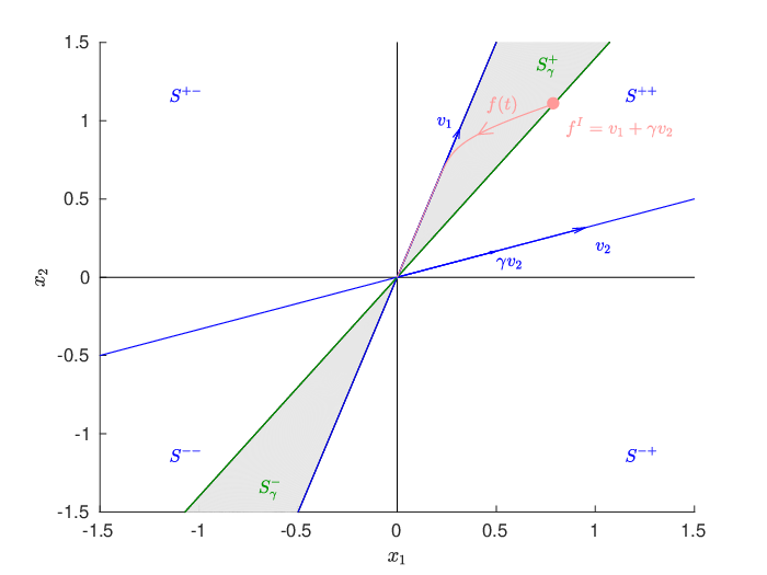
Considering a matrix 𝐂∈ℝ2×2\mathbf{C}\in\mathbb{R}^{2\times 2} with two distinct real eigenvalues λ1<λ2\lambda_{1}<\lambda_{2} and real eigenvectors v1v_{1} and v2v_{2}, then the associated eigenspaces span⁡{v1}\linspan\{v_{1}\} and span⁡{v2}\linspan\{v_{2}\} dissect the plane into four sectors

(4.3) 𝒮±⁣∓:={z1v1+z2v2|z1∈ℝ±,z2∈ℝ∓},\mathcal{S}^{\pm\mp}:=\{z_{1}v_{1}+z_{2}v_{2}\ |\ z_{1}\in\mathbb{R}^{\pm}\,,\ z_{2}\in\mathbb{R}^{\mp}\}\,,

see Fig. 1. A solution f⁡(t)f(t) of ODE (2.1) starting in an eigenspace will approach the origin in a straight line, such that

(4.4) ‖f⁡(t)‖22=e−2​λj𝐂​t​‖fI‖22∀t≥0.\|f(t)\|^{2}_{2}=e^{-2\lambda_{j}^{\mathbf{C}}t}\|f^{I}\|^{2}_{2}\qquad\forall t\geq 0\,.

If a solution starts instead in one of the four (open) sectors 𝒮±⁣∓\mathcal{S}^{\pm\mp}, it will remain in that sector while approaching the origin. In fact, since λ1𝐂<λ2𝐂\lambda_{1}^{\mathbf{C}}<\lambda_{2}^{\mathbf{C}}, if fI=z1​(v1+γ​v2)f^{I}=z_{1}(v_{1}+\gamma v_{2}) for some z1∈ℝ∖{0}z_{1}\in\mathbb{R}\setminus\{0\} and γ∈ℝ\gamma\in\mathbb{R}, then the solution

f⁡(t)=z1​(e−λ1𝐂​t​v1+γ​e−λ2𝐂​t​v2)=z1​e−λ1𝐂​t​(v1+γ​e−(λ2𝐂−λ1𝐂)​t​v2)f(t)=z_{1}\big(e^{-\lambda_{1}^{\mathbf{C}}t}v_{1}+\gamma e^{-\lambda_{2}^{\mathbf{C}}t}v_{2}\big)=z_{1}e^{-\lambda_{1}^{\mathbf{C}}t}\big(v_{1}+\gamma e^{-(\lambda_{2}^{\mathbf{C}}-\lambda_{1}^{\mathbf{C}})t}v_{2}\big)

of the ODE (2.1) will remain in the sector

(4.5) 𝒮γ±:={z1(v1+z2v2)|z1∈ℝ±,z2∈[min(0,γ),max(0,γ)]},\mathcal{S}^{\pm}_{\gamma}:=\{z_{1}(v_{1}+z_{2}v_{2})\ |\ z_{1}\in\mathbb{R}^{\pm}\,,\ z_{2}\in[\min(0,\gamma),\max(0,\gamma)]\}\,,

see Fig. 1.

Refer to caption
Figure 1. The blue (black) lines are the eigenspaces span⁡{v1}\linspan\{v_{1}\} and span⁡{v2}\linspan\{v_{2}\} of matrix 𝐂\mathbf{C}. The red (grey) curve is a solution f⁡(t)f(t) of the ODE (2.1) with initial datum fIf^{I}. The shaded regions are the sectors Sγ+S^{+}_{\gamma}, Sγ−S^{-}_{\gamma} with the choice γ=1/2\gamma=1/2. Note: The curves are colored only in the electronic version of this article.

For a fixed fI=z1​(v1+γ​v2)f^{I}=z_{1}(v_{1}+\gamma v_{2}), let 𝒮\mathcal{S} be the corresponding sector 𝒮γ±\mathcal{S}^{\pm}_{\gamma}. Then estimate (2.5) can be improved as follows

(4.6) ‖f⁡(t)‖22≤1λmin,𝒮𝐏​‖f⁡(t)‖𝐏2≤e−2​μ​tλmin,𝒮𝐏​‖fI‖𝐏2≤c𝒮​(𝐏)​e−2​μ​t​‖fI‖22,t≥0,\|f(t)\|^{2}_{2}\leq\frac{1}{\lambda^{\mathbf{P}}_{\min,\,\mathcal{S}}}\|f(t)\|^{2}_{\mathbf{P}}\leq\frac{e^{-2\mu t}}{\lambda^{\mathbf{P}}_{\min,\,\mathcal{S}}}\|f^{I}\|^{2}_{\mathbf{P}}\leq c_{\mathcal{S}}(\mathbf{P})\,e^{-2\mu t}\|f^{I}\|^{2}_{2}\,,\quad t\geq 0\,,

where

(4.7) λmin,𝒮𝐏:=infx∈𝒮⟨x,𝐏​x⟩⟨x,x⟩,λi​n​i​t,𝒮𝐏:=⟨fI,𝐏​fI⟩⟨fI,fI⟩,c𝒮​(𝐏):=λi​n​i​t,𝒮𝐏λmin,𝒮𝐏.\lambda^{\mathbf{P}}_{\min,\,\mathcal{S}}:=\inf_{x\in\mathcal{S}}\frac{\langle{x},\,{\mathbf{P}x}\rangle}{\langle{x},\,{x}\rangle}\,,\quad\lambda^{\mathbf{P}}_{init,\,\mathcal{S}}:=\frac{\langle{f^{I}},\,{\mathbf{P}f^{I}}\rangle}{\langle{f^{I}},\,{f^{I}}\rangle}\,,\quad c_{\mathcal{S}}(\mathbf{P}):=\frac{\lambda^{\mathbf{P}}_{init,\,\mathcal{S}}}{\lambda^{\mathbf{P}}_{\min,\,\mathcal{S}}}\,.

Note that, in the definition of λi​n​i​t,𝒮𝐏\lambda^{\mathbf{P}}_{init,\,\mathcal{S}} the sector 𝒮∈{𝒮γ±|γ∈ℝ}\mathcal{S}\in\left\{\mathcal{S}_{\gamma}^{\pm}\big|\gamma\in\mathbb{R}\right\} also determines corresponding initial conditions fI∈∂𝒮f^{I}\in\partial\mathcal{S} via fI=z1​(v1+γ​v2)f^{I}=z_{1}(v_{1}+\gamma v_{2}) (up to the constant z1≠0z_{1}\neq 0 which drops out in λi​n​i​t,𝒮𝐏\lambda^{\mathbf{P}}_{init,\,\mathcal{S}}).

For (4.6) to hold for all trajectories and one fixed constant on the right hand side, we have to take the supremum over all initial conditions or, equivalently, over all sectors 𝒮∈{𝒮γ±|γ∈ℝ}\mathcal{S}\in\left\{\mathcal{S}_{\gamma}^{\pm}\big|\gamma\in\mathbb{R}\right\}. Although fI=z2​v2f^{I}=z_{2}v_{2} is not included in any sector 𝒮γ+\mathcal{S}_{\gamma}^{+}, its corresponding multiplicative constant 1 (see (4.4)) is still covered. Then, the minimal multiplicative constant in (3.1) using (4.6) is

(4.8) c~=inf𝐏sup𝒮c𝒮​(𝐏),\widetilde{c}=\sqrt{\inf_{\mathbf{P}}\,\sup_{\mathcal{S}}\,c_{\mathcal{S}}(\mathbf{P})}\,,

where 𝐏\mathbf{P} ranges over all matrices of the form (2.3).

Step 1 (computation of λmin,𝒮γ+𝐏\lambda_{\min,\,\mathcal{S}^{+}_{\gamma}}^{\mathbf{P}} for γ\gamma fixed): To find an explicit expression for this minimal constant cc, we first determine c𝒮​(𝐏)c_{\mathcal{S}}(\mathbf{P}) for a given admissible matrix 𝐏\mathbf{P}. As an example of sectors, we consider only 𝒮γ+\mathcal{S}^{+}_{\gamma} for fixed γ≤0\gamma\leq 0 and compute

λmin,𝒮γ+𝐏\displaystyle\lambda_{\min,\,\mathcal{S}^{+}_{\gamma}}^{\mathbf{P}} =infx∈𝒮γ+⟨x,𝐏​x⟩‖x‖2=infz1∈ℝ+,z2∈[γ,0]⟨z1​(v1+z2​v2),𝐏⁡(z1​(v1+z2​v2))⟩‖z1​(v1+z2​v2)‖2\displaystyle=\inf_{x\in\mathcal{S}^{+}_{\gamma}}\frac{\langle{x},\,{\mathbf{P}x}\rangle}{\|{x}\|^{2}}=\inf_{z_{1}\in\mathbb{R}^{+},\,z_{2}\in[\gamma,0]}\frac{\langle{z_{1}(v_{1}+z_{2}v_{2})},\,{\mathbf{P}(z_{1}(v_{1}+z_{2}v_{2}))}\rangle}{\|{z_{1}(v_{1}+z_{2}v_{2})}\|^{2}}
=infz2∈[γ,0]⟨v1+z2​v2,𝐏⁡(v1+z2​v2)⟩‖v1+z2​v2‖2.\displaystyle=\inf_{z_{2}\in[\gamma,0]}\frac{\langle{v_{1}+z_{2}v_{2}},\,{\mathbf{P}(v_{1}+z_{2}v_{2})}\rangle}{\|{v_{1}+z_{2}v_{2}}\|^{2}}\,.

This also shows that λmin,𝒮γ+𝐏=λmin,𝒮γ−𝐏\lambda_{\min,\,\mathcal{S}^{+}_{\gamma}}^{\mathbf{P}}=\lambda_{\min,\,\mathcal{S}^{-}_{\gamma}}^{\mathbf{P}} for any fixed γ∈ℝ\gamma\in\mathbb{R}. Next, we use the result of Lemma 3.1 and (3.6), stating that the only admissible matrices are 𝐏=𝐖​diag⁡(b1,b2)​𝐖∗\mathbf{P}=\mathbf{W}\diag(b_{1},b_{2})\mathbf{W}^{*} for b1,b2>0b_{1},b_{2}>0. Since c𝒮​(b​𝐏)=c𝒮​(𝐏)c_{\mathcal{S}}(b\mathbf{P})=c_{\mathcal{S}}(\mathbf{P}) for all b>0b>0, we consider w.l.o.g. b1=1/bb_{1}=1/b and b2=bb_{2}=b for b>0b>0. Then, we deduce

λmin,𝒮γ+𝐏\displaystyle\lambda_{\min,\,\mathcal{S}^{+}_{\gamma}}^{\mathbf{P}} =infz∈[γ,0]⟨v1+z​v2,𝐏⁡(v1+z​v2)⟩‖v1+z​v2‖2\displaystyle=\inf_{z\in[\gamma,0]}\frac{\langle{v_{1}+zv_{2}},\,{\mathbf{P}(v_{1}+zv_{2})}\rangle}{\|{v_{1}+zv_{2}}\|^{2}}
=infz∈[γ,0]⟨𝐖∗​(v1+z​v2),diag⁡(1/b,b)​𝐖∗​(v1+zv2)⟩‖v1+z​v2‖2.\displaystyle=\inf_{z\in[\gamma,0]}\frac{\langle{\mathbf{W}^{*}(v_{1}+zv_{2})},\,{\diag(1/b,b)\mathbf{W}^{*}(v_{1}+zv_{2})}\rangle}{\|{v_{1}+zv_{2}}\|^{2}}\,.

In our case of a real matrix 𝐂\mathbf{C} with distinct real eigenvalues, the left and right eigenvectors are related as follows: Up to a change of orientation, ⟨wj,vk⟩=δj​k\langle{w_{j}},\,{v_{k}}\rangle=\delta_{jk} (j,k∈{1,2}j,k\in\{1,2\}). Considering ⟨wj,vj⟩=1\langle{w_{j}},\,{v_{j}}\rangle=1 for j=1,2j=1,2, implies that the vectors wjw_{j} and vjv_{j} can be normalized simultaneously only if matrix 𝐂\mathbf{C} is symmetric. Therefore, using a coordinate system such that the normalized eigenvectors of 𝐂∗\mathbf{C}^{*} are given as (3.7) and 𝐕:=(v1|v2)=(𝐖∗)−1\mathbf{V}:=(v_{1}|v_{2})=(\mathbf{W}^{*})^{-1} yields

v1=11−α2(1−α2−α),v2=11−α2(01)for α in (3.7).v_{1}=\frac{1}{\sqrt{1-\alpha^{2}}}\begin{pmatrix}\sqrt{1-\alpha^{2}}\\ -\alpha\end{pmatrix}\,,\quad v_{2}=\frac{1}{\sqrt{1-\alpha^{2}}}\begin{pmatrix}0\\ 1\end{pmatrix}\quad\text{for $\alpha$ in\penalty\ \eqref{eigenvectors:newBasis}.}

Finally, we obtain

λmin,𝒮γ+𝐏=infz∈[γ,0]⟨𝐖∗​(v1+z​v2),diag⁡(1/b,b)​𝐖∗​(v1+zv2)⟩‖v1+z​v2‖2=infz∈[γ,0]g⁡(z)\lambda_{\min,\,\mathcal{S}^{+}_{\gamma}}^{\mathbf{P}}=\inf_{z\in[\gamma,0]}\frac{\langle{\mathbf{W}^{*}(v_{1}+zv_{2})},\,{\diag(1/b,b)\mathbf{W}^{*}(v_{1}+zv_{2})}\rangle}{\|{v_{1}+zv_{2}}\|^{2}}=\inf_{z\in[\gamma,0]}g(z)

and λi​n​i​t,𝒮γ+𝐏=g⁡(γ)\lambda^{\mathbf{P}}_{init,\,\mathcal{S}^{+}_{\gamma}}=g(\gamma) with

(4.9) g⁡(z):=(1−α2)​(1b+b​z2)1−2​α​z+z2.g(z):=\frac{(1-\alpha^{2})\,(\frac{1}{b}+bz^{2})}{1-2\alpha z+z^{2}}\,.

Step 2 (extrema of the function gg): The function gg has local extrema at

z±=12​α​b​(b−1b±(b−1b)2+4​α2)z_{\pm}=\frac{1}{2\alpha b}\Big(b-\frac{1}{b}\pm\sqrt{\big(b-\frac{1}{b}\big)^{2}+4\alpha^{2}}\Big)

which satisfy z−<0<z+z_{-}<0<z_{+}. Writing g′​(z)=h1​(z)/h2​(z)g^{\prime}(z)=h_{1}(z)/h_{2}(z) with h1​(z):=(−2​α​b​z2+2​(b−1b)​z+2b​α)h_{1}(z):=\big(-2\alpha bz^{2}+2\big(b-\frac{1}{b}\big)z+\frac{2}{b}\alpha\big) and h2​(z):=(1−2​α​z+z2)2/(1−α2)>0h_{2}(z):=(1-2\alpha z+z^{2})^{2}/(1-\alpha^{2})>0, we derive

g′′​(z±)=h1′​(z±)h2​(z±)=∓2​1h2​(z±)​(b−1b)2+4​α2.g^{\prime\prime}(z_{\pm})=\frac{h_{1}^{\prime}(z_{\pm})}{h_{2}(z_{\pm})}=\mp 2\frac{1}{h_{2}(z_{\pm})}\sqrt{\big(b-\frac{1}{b}\big)^{2}+4\alpha^{2}}\,.

In fact, the function gg attains its global minimum on ℝ\mathbb{R} (and on ℝ0−\mathbb{R}_{0}^{-}) at z−z_{-}, and its global maximum on ℝ\mathbb{R} at z+z_{+}. The global supremum of g⁡(z)g(z) on ℝ−\mathbb{R}^{-} exists and satisfies

supz∈ℝ−g⁡(z)={g⁡(0)=(1−α2)/bif ​b∈(0,1),g⁡(0)=limz→−∞g⁡(z)=1−α2if ​b=1,limz→−∞g⁡(z)=(1−α2)​bif ​b∈(1,∞).\sup_{z\in\mathbb{R}^{-}}g(z)=\begin{cases}g(0)=(1-\alpha^{2})/b&\text{if }b\in(0,1)\,,\\ g(0)=\lim_{z\to-\infty}g(z)=1-\alpha^{2}&\text{if }b=1\,,\\ \lim_{z\to-\infty}g(z)=(1-\alpha^{2})b&\text{if }b\in(1,\infty)\,.\end{cases}

Step 3 (optimization of c𝒮γ±​(𝐏)c_{\mathcal{S}^{\pm}_{\gamma}}(\mathbf{P}) w.r.t. γ\gamma): We obtain

c𝒮γ±​(𝐏⁡(b))=g⁡(γ)λmin,𝒮γ+𝐏⁡(b)={1if ​z−≤γ<0,g⁡(γ)/g⁡(z−)if ​γ≤z−.c_{\mathcal{S}^{\pm}_{\gamma}}(\mathbf{P}(b))=\frac{g(\gamma)}{\lambda_{\min,\,\mathcal{S}^{+}_{\gamma}}^{\mathbf{P}(b)}}=\begin{cases}1&\text{if }z_{-}\leq\gamma<0\,,\\ g(\gamma)/g(z_{-})&\text{if }\gamma\leq z_{-}\,.\end{cases}

Finally, we derive

(4.10) supγ∈ℝ−c𝒮γ±​(𝐏⁡(b))=limγ→−∞g⁡(γ)g⁡(z−)=(1−α2)​bg⁡(z−),\sup_{\gamma\in\mathbb{R}^{-}}c_{\mathcal{S}^{\pm}_{\gamma}}(\mathbf{P}(b))=\lim_{\gamma\to-\infty}\frac{g(\gamma)}{g(z_{-})}=\frac{(1-\alpha^{2})b}{g(z_{-})}\,,

and in a similar way,

(4.11) supγ∈ℝ+c𝒮γ±​(𝐏⁡(b))=g⁡(z+)g⁡(0)=b​g​(z+)1−α2.\sup_{\gamma\in\mathbb{R}^{+}}c_{\mathcal{S}^{\pm}_{\gamma}}(\mathbf{P}(b))=\frac{g(z_{+})}{g(0)}=\frac{bg(z_{+})}{1-\alpha^{2}}\,.

To finish this analysis we note that c𝒮0±​(𝐏​(b))=1c_{\mathcal{S}^{\pm}_{0}}(\mathbf{P}(b))=1, due to (4.4) and fI=z1​v1f^{I}=z_{1}v_{1}.

Step 4 (minimization of sup𝒮c𝒮​(𝐏)\sup_{\mathcal{S}}\,c_{\mathcal{S}}(\mathbf{P}) w.r.t. 𝐏\mathbf{P}): We obtain

inf𝐏sup𝒮c𝒮​(𝐏)=infb∈(0,∞)supγ∈ℝc𝒮γ±​(𝐏⁡(b))=infb∈(0,∞)max⁡{(1−α2)​bg⁡(z−), 1,b​g​(z+)1−α2}.\inf_{\mathbf{P}}\,\sup_{\mathcal{S}}\,c_{\mathcal{S}}(\mathbf{P})=\inf_{b\in(0,\infty)}\sup_{\gamma\in\mathbb{R}}c_{\mathcal{S}^{\pm}_{\gamma}}(\mathbf{P}(b))\\ =\inf_{b\in(0,\infty)}\max\Big\{\frac{(1-\alpha^{2})b}{g(z_{-})},\,1,\,\frac{bg(z_{+})}{1-\alpha^{2}}\Big\}\,.

Taking into account the bb-dependence of z±z_{\pm}, the functions (1−α2)​bg⁡(z−)\frac{(1-\alpha^{2})b}{g(z_{-})} and b​g​(z+)1−α2\frac{bg(z_{+})}{1-\alpha^{2}} are monotone increasing in bb, since

∂∂b​(1−α2)​bg⁡(z−)>0,∂∂b​b​g​(z+)1−α2>0.\frac{\partial}{\partial b}\frac{(1-\alpha^{2})b}{g(z_{-})}>0\,,\qquad\frac{\partial}{\partial b}\frac{bg(z_{+})}{1-\alpha^{2}}>0\,.

Therefore we have to study their limits as b→0b\to 0: We derive

(4.12) limb→0(1−α2)​bg⁡(z−)=1usinglimb→0z−​(b)=−∞,limb→0b​g​(z+)1−α2=11−α2>1usinglimb→0z+​(b)=α.\begin{split}&\lim_{b\to 0}\frac{(1-\alpha^{2})b}{g(z_{-})}=1\qquad\qquad\text{using}\quad\lim_{b\to 0}z_{-}(b)=-\infty\,,\\ &\lim_{b\to 0}\frac{bg(z_{+})}{1-\alpha^{2}}=\frac{1}{1-\alpha^{2}}>1\qquad\text{using}\quad\lim_{b\to 0}z_{+}(b)=\alpha\,.\end{split}

Hence, infb∈(0,∞)supγ∈ℝc𝒮γ±​(𝐏⁡(b))\inf_{b\in(0,\infty)}\,\sup_{\gamma\in\mathbb{R}}\,c_{\mathcal{S}^{\pm}_{\gamma}}(\mathbf{P}(b)) is realized by the sector 𝒮γ±\mathcal{S}^{\pm}_{\gamma} with γ=z+​(b)>0\gamma=z_{+}(b)>0 and in the limit b→0b\to 0. Altogether we obtain

c~=inf𝐏sup𝒮c𝒮​(𝐏)=11−α2,\widetilde{c}=\sqrt{\inf_{\mathbf{P}}\,\sup_{\mathcal{S}}\,c_{\mathcal{S}}(\mathbf{P})}=\frac{1}{\sqrt{1-\alpha^{2}}}\,,

where the first equality holds since we discussed all solutions. This finishes the proof.

Step 5: Finally we have to verify that c~\widetilde{c} is minimal in (3.1). We shall show that it is attained asymptotically (as t→∞t\to\infty) for a concrete trajectory: For fixed b∈(0,∞)b\in(0,\infty), the minimal multiplicative constant in (4.6) is attained for the solution with initial datum fI=v1+z+​(b)​v2=y+𝐏⁡(b)f^{I}=v_{1}+z_{+}(b)v_{2}=y_{+}^{\mathbf{P}(b)}, which is the eigenvector pertaining to the largest eigenvalue of 𝐏⁡(b)\mathbf{P}(b) (cp. to the proof of Theorem 3.7). The formula for fIf^{I} holds since sup𝒮c𝒮​(𝐏⁡(b))=b​g​(z+​(b))/(1−α2)\sup_{\mathcal{S}}\,c_{\mathcal{S}}(\mathbf{P}(b))=bg(z_{+}(b))/(1-\alpha^{2}). This can be verified by a direct comparison of (4.10) and (4.11). For bb small it also follows from (4.12). In the limit b→0b\to 0, 𝐏⁡(b)\mathbf{P}(b) in (3.9) approaches a multiple of w1⊗w1∗w_{1}\otimes w_{1}^{*} and

fI=v1+z+​(b)​v2⟶v1+α​v2=w1.f^{I}=v_{1}+z_{+}(b)v_{2}\longrightarrow v_{1}+\alpha v_{2}=w_{1}\,.

The solution f⁡(t)f(t) of the ODE (2.1) with fI=w1f^{I}=w_{1} satisfies

(4.13) f⁡(t)=e−𝐂​t​w1=𝐕​(e−λ1​t00e−λ2​t)​𝐖∗​w1=e−λ1​t​v1+α​e−λ2​t​v2.f(t)=e^{-\mathbf{C}t}w_{1}=\mathbf{V}\begin{pmatrix}e^{-\lambda_{1}t}&0\\ 0&e^{-\lambda_{2}t}\end{pmatrix}\mathbf{W}^{*}w_{1}=e^{-\lambda_{1}t}v_{1}+\alpha e^{-\lambda_{2}t}v_{2}\,.

This implies

eℜ⁡λ1​t​‖f⁡(t)‖2‖fI‖2≤‖v1+α​e−ℜ⁡(λ2−λ1)​t​v2‖2⟶t→∞‖v1‖2=11−α2e^{\Re\lambda_{1}t}\frac{\|f(t)\|_{2}}{\|f^{I}\|_{2}}\leq\|v_{1}+\alpha e^{-\Re(\lambda_{2}-\lambda_{1})t}v_{2}\|_{2}\stackrel{{\scriptstyle t\to\infty}}{{\longrightarrow}}\|v_{1}\|_{2}=\tfrac{1}{\sqrt{1-\alpha^{2}}}

and it finishes the proof. ∎ ∎

After the analysis in Theorems 3.7 and 4.1, we are left with the case of a matrix 𝐂∈ℂ2×2\mathbf{C}\in\mathbb{C}^{2\times 2} with eigenvalues λ1\lambda_{1} and λ2\lambda_{2} such that the real and imaginary parts are distinct. This case can not occur for real matrices 𝐂\mathbf{C}. The proof of Lemma 3.3 gives an upper bound 1+α1−α\sqrt{\tfrac{1+\alpha}{1-\alpha}} for the multiplicative constant in (3.1). On the other hand, the solution f⁡(t)f(t) of the ODE (2.1) with fI=w1f^{I}=w_{1} satisfies (4.13), hence,

‖f⁡(t)‖22\displaystyle\|f(t)\|_{2}^{2} =e−2​ℜ⁡λ1​t​‖v1+α​e−(λ2−λ1)​t​v2‖22\displaystyle=e^{-2\Re\lambda_{1}t}\|v_{1}+\alpha e^{-(\lambda_{2}-\lambda_{1})t}v_{2}\|_{2}^{2}
=11−α2​e−2​ℜ⁡λ1​t​(1−2​α2​e−ℜ⁡(λ2−λ1)​t​cos⁡(ℑ⁡(λ2−λ1)​t)+α2​e−2​ℜ⁡(λ2−λ1)​t).\displaystyle=\tfrac{1}{1-\alpha^{2}}e^{-2\Re\lambda_{1}t}\Big(1-2\alpha^{2}e^{-\Re(\lambda_{2}-\lambda_{1})t}\cos\big(\Im(\lambda_{2}-\lambda_{1})t\big)+\alpha^{2}e^{-2\Re(\lambda_{2}-\lambda_{1})t}\Big)\,.

The expression in the bracket is bigger than 1, e.g. at time t=π/ℑ⁡(λ2−λ1)t=\pi/\Im(\lambda_{2}-\lambda_{1}). Thus the minimal multiplicative constant cc is definitely bigger than 11−α2\tfrac{1}{\sqrt{1-\alpha^{2}}}, which is the best constant for ℑ⁡λ1=ℑ⁡λ2\Im\lambda_{1}=\Im\lambda_{2} (see Theorem 4.1).

Next, we derive the upper and lower envelopes for the norm of solutions f⁡(t)f(t) of ODE (2.1) in order to determine the sharp constant cc. For a diagonalizable matrix 𝐂∈ℂ2×2\mathbf{C}\in\mathbb{C}^{2\times 2} with λ1𝐂=λ2𝐂\lambda_{1}^{\mathbf{C}}=\lambda_{2}^{\mathbf{C}} it holds that ‖f⁡(t)‖2=e−ℜ⁡λ1𝐂​t​‖fI‖2\|f(t)\|_{2}=e^{-\Re\lambda_{1}^{\mathbf{C}}t}\|f^{I}\|_{2}. And for the general case we have:

Proposition 4.2.

Let 𝐂∈ℂ2×2\mathbf{C}\in\mathbb{C}^{2\times 2} be a diagonalizable, positive stable matrix with eigenvalues λ1𝐂≠λ2𝐂\lambda_{1}^{\mathbf{C}}\neq\lambda_{2}^{\mathbf{C}}, and associated eigenvectors v1v_{1} and v2v_{2}, resp. Then the norm of solutions f⁡(t)f(t) of ODE (2.1) satisfies

h−​(t)​‖fI‖22≤‖f⁡(t)‖22≤h+​(t)​‖fI‖22,∀t≥0,h_{-}(t)\|f^{I}\|^{2}_{2}\leq\|f(t)\|^{2}_{2}\leq h_{+}(t)\|f^{I}\|^{2}_{2}\,,\qquad\forall t\geq 0\,,

where the envelopes h±​(t)h_{\pm}(t) are given by

h±​(t):=e−2​ℜ⁡λ1𝐂​t​m±​(t)h_{\pm}(t):=e^{-2\Re\lambda_{1}^{\mathbf{C}}t}m_{\pm}(t)

with

m±​(t):=±e−γ​t​((cosh⁡(γ​t)−α2​cos⁡(δ​t))2(1−α2)2−1±(cosh⁡(γ​t)−α2​cos⁡(δ​t))1−α2),m_{\pm}(t):=\pm e^{-\gamma t}\Big(\sqrt{\frac{\big(\cosh(\gamma t)-\alpha^{2}\cos(\delta t)\big)^{2}}{(1-\alpha^{2})^{2}}-1}\pm\frac{\big(\cosh(\gamma t)-\alpha^{2}\cos(\delta t)\big)}{1-\alpha^{2}}\Big)\,,

where γ:=ℜ⁡(λ2𝐂−λ1𝐂)\gamma:=\Re(\lambda_{2}^{\mathbf{C}}-\lambda_{1}^{\mathbf{C}}), δ:=ℑ⁡(λ2𝐂−λ1𝐂)\delta:=\Im(\lambda_{2}^{\mathbf{C}}-\lambda_{1}^{\mathbf{C}}), α:=|⟨v1‖v1‖,v2‖v2‖⟩|\alpha:=\Big|\Big\langle{\frac{v_{1}}{\|v_{1}\|}}\,,{\frac{v_{2}}{\|v_{2}\|}}\Big\rangle\Big| and α∈[0,1)\alpha\in[0,1).

While the rest of the article is based on estimating Lyapunov functionals, the following proof will use the explicit solution formula of the ODE.

Proof.

We use again the unitary transformation as in the proof of Lemma 3.3, such that the eigenvectors w1w_{1} and w2w_{2} of 𝐂∗\mathbf{C}^{*} are given in (3.7). If f⁡(t)f(t) is a solution of (2.1), then f~​(t)=eλ1𝐂​t​f​(t)\tilde{f}(t)=e^{\lambda_{1}^{\mathbf{C}}t}f(t) satisfies

(4.14) dd⁡t​f~​(t)=−𝐂~​f~​(t),f~​(0)=fI,\frac{\,\operatorname{d}\!}{\,\operatorname{d}\!t}\tilde{f}(t)=-\widetilde{\mathbf{C}}\tilde{f}(t)\,,\quad\tilde{f}(0)=f^{I}\,,

with

𝐂~=(𝐂−λ1𝐂​𝐈)=(𝐖∗)−1​(000λ2𝐂−λ1𝐂)​𝐖∗.\widetilde{\mathbf{C}}=(\mathbf{C}-\lambda_{1}^{\mathbf{C}}\mathbf{I})=(\mathbf{W}^{*})^{-1}\begin{pmatrix}0&0\\ 0&\lambda_{2}^{\mathbf{C}}-\lambda_{1}^{\mathbf{C}}\end{pmatrix}\mathbf{W}^{*}\,.

The explicit solution f~​(t)\tilde{f}(t) of (4.14) is

f~​(t)=(𝐖∗)−1​(100e−(γ+i​δ)​t)​𝐖∗​fI=(f1Iα1−α2​(e−(γ+i​δ)​t−1)​f1I+e−(γ+i​δ)​t​f2I),\tilde{f}(t)=(\mathbf{W}^{*})^{-1}\begin{pmatrix}1&0\\ 0&e^{-(\gamma+i\delta)t}\end{pmatrix}\mathbf{W}^{*}f^{I}=\begin{pmatrix}f^{I}_{1}\\ \tfrac{\alpha}{\sqrt{1-\alpha^{2}}}(e^{-(\gamma+i\delta)t}-1)f^{I}_{1}+e^{-(\gamma+i\delta)t}f^{I}_{2}\end{pmatrix}\,,

where γ=ℜ⁡(λ2𝐂−λ1𝐂)\gamma=\Re(\lambda_{2}^{\mathbf{C}}-\lambda_{1}^{\mathbf{C}}) and δ=ℑ⁡(λ2𝐂−λ1𝐂)\delta=\Im(\lambda_{2}^{\mathbf{C}}-\lambda_{1}^{\mathbf{C}}). If the initial data fIf^{I} lies in ℝ×ℂ\mathbb{R}\times\mathbb{C} then the solution will satisfy f~​(t)∈ℝ×ℂ\tilde{f}(t)\in\mathbb{R}\times\mathbb{C} for all t≥0t\geq 0. The multiplication with f1I¯/|f1I|\overline{f^{I}_{1}}/|f^{I}_{1}| is another unitary transformation and does not change the norm. Therefore, to compute the envelope for the norm of solutions f~​(t)\tilde{f}(t) of ODE (4.14) we assume w.l.o.g. that

(4.15) fϕ,θI=(cos⁡(ϕ)sin⁡(ϕ)​ei​θ)∈ℝ×ℂ,where ​ϕ,θ∈[0,2​π),f^{I}_{\phi,\theta}=\begin{pmatrix}\cos(\phi)\\ \sin(\phi)e^{i\theta}\end{pmatrix}\in\mathbb{R}\times\mathbb{C}\,,\qquad\text{where }\phi,\theta\in[0,2\pi)\,,

such that ‖fϕ,θI‖=1\|f^{I}_{\phi,\theta}\|=1. We consider the solution f~ϕ,θ​(t)\tilde{f}_{\phi,\theta}(t) for (4.14) with fI=fϕ,θIf^{I}=f^{I}_{\phi,\theta}. To compute the envelopes (for fixed tt), we solve ∂ϕ‖f~ϕ,θ‖2=0\partial_{\phi}\|\tilde{f}_{\phi,\theta}\|^{2}=0 and ∂θ‖f~ϕ,θ‖2=0\partial_{\theta}\|\tilde{f}_{\phi,\theta}\|^{2}=0 in terms of ϕ\phi and θ\theta. Evaluating ‖f~ϕ,θ​(t)‖2\|\tilde{f}_{\phi,\theta}(t)\|^{2} at ϕ=ϕ⁡(t)\phi=\phi(t) and θ=θ⁡(t)\theta=\theta(t) yields the envelopes for the norm of solutions f~​(t)\tilde{f}(t) of ODE (4.14). Consequently, we derive the envelopes h±​(t)​‖fI‖2h_{\pm}(t)\|f^{I}\|^{2} for the original problem, since ‖f⁡(t)‖2=e−ℜ⁡λ1𝐂​t​‖f~​(t)‖2\|f(t)\|_{2}=e^{-\Re\lambda_{1}^{\mathbf{C}}t}\|\tilde{f}(t)\|_{2}. ∎ ∎

Corollary 4.3.

Let 𝐂∈ℂ2×2\mathbf{C}\in\mathbb{C}^{2\times 2} be a diagonalizable, positive stable matrix. Then the minimal multiplicative constant cc in (3.1) for the ODE (2.1) is given by

(4.16) c=supt≥0m+​(t),c=\sqrt{\sup_{t\geq 0}m_{+}(t)}\,,

where m+​(t)m_{+}(t) is the function given in Proposition 4.2.

In general we could not find an explicit formula for supt≥0m+​(t)\sup_{t\geq 0}m_{+}(t).

5. A Family of Decay Estimates for Hypocoercive ODEs

In this section we shall illustrate the interdependence of maximizing the decay rate λ\lambda and minimizing the multiplicative constant cc in estimates like (3.1). For the ODE-system (2.1), the procedure described in Remark 1.2(b) yields the optimal bound for large time, with the sharp decay rate μ:=min{ℜ(λ)|λ\mu:=\min\{\Re(\lambda)|\lambda is an eigenvalue of 𝐂}\mathbf{C}\}. But for non-coercive 𝐂\mathbf{C} we must have c>1c>1. Hence, such a bound cannot be sharp for short time. As a counterexample we consider the simple energy estimate (obtained by premultiplying (2.1) with f∗f^{*})

‖f⁡(t)‖2≤e−μs​t​‖fI‖2,t≥0,\|f(t)\|_{2}\leq e^{-\mu_{s}t}\|f^{I}\|_{2}\,,\quad t\geq 0\,,

with 𝐂s:=12​(𝐂+𝐂∗)\mathbf{C}_{s}:=\frac{1}{2}(\mathbf{C}+\mathbf{C}^{*}) and μs:=min{λ|λ\mu_{s}:=\min\{\lambda|\lambda is an eigenvalue of 𝐂s}\mathbf{C}_{s}\}.

The goal of this section is to derive decay estimates for (2.1) with rates in between this weakest rate μs\mu_{s} and the optimal rate μ\mu from (2.5). It holds that μs≤μ\mu_{s}\leq\mu. At the same time we shall also present lower bounds on ‖f⁡(t)‖2\|f(t)\|_{2}. The energy method again provides the simplest example of it, in the form

‖f⁡(t)‖2≥e−νs​t​‖fI‖2,t≥0,\|f(t)\|_{2}\geq e^{-\nu_{s}t}\|f^{I}\|_{2}\,,\quad t\geq 0\,,

with νs:=max{λ|λ\nu_{s}:=\max\{\lambda|\lambda is an eigenvalue of 𝐂s}\mathbf{C}_{s}\}. Clearly, estimates with decay rates outside of [μs,νs][\mu_{s},\nu_{s}] are irrelevant.

We present our main result only for the two-dimensional case, as the best multiplicative constant is not yet known explicitly in higher dimensions (cf. §3):

Proposition 5.1.

Let 𝐂∈ℂ2×2\mathbf{C}\in\mathbb{C}^{2\times 2} be a diagonalizable positive stable matrix with spectral gap μ:=min{ℜ(λj𝐂)|j=1,2}\mu:=\min\{\Re(\lambda_{j}^{\mathbf{C}})|\,j=1,2\}. Then, all solutions to (2.1) satisfy the following upper and lower bounds:

  • a)
    (5.1) ‖f⁡(t)‖2≤c1​(μ~)​e−μ~​t​‖fI‖2,t≥0,μs≤μ~≤μ,\|f(t)\|_{2}\leq c_{1}(\tilde{\mu})\,e^{-\tilde{\mu}t}\|f^{I}\|_{2}\,,\quad t\geq 0\,,\quad\mu_{s}\leq\tilde{\mu}\leq\mu\,,

    with

    c12​(μ~)=κmin​(β⁡(μ~))c_{1}^{2}(\tilde{\mu})=\kappa_{\min}(\beta(\tilde{\mu}))

    given explicitly in (5.8) below. There, α∈[0,1)\alpha\in[0,1) is the cos\cos of the (minimal) angle of the eigenvectors of 𝐂∗\mathbf{C}^{*} (cf. the proof of Lemma 3.3), and β⁡(μ~)=max⁡(−α,−β0)\beta(\tilde{\mu})=\max(-\alpha,-\beta_{0}), with β0\beta_{0} defined in (5.6), (5.7) below.

  • b)
    (5.2) ‖f⁡(t)‖2≥c2​(μ~)​e−μ~​t​‖fI‖2,t≥0,ν≤μ~≤νs,\|f(t)\|_{2}\geq c_{2}(\tilde{\mu})\,e^{-\tilde{\mu}t}\|f^{I}\|_{2}\,,\quad t\geq 0\,,\quad\nu\leq\tilde{\mu}\leq\nu_{s}\,,

    with ν:=max{ℜ(λj𝐂)|j=1,2}\nu:=\max\{\Re(\lambda_{j}^{\mathbf{C}})|\,j=1,2\}. The maximal constant

    c22​(μ~)=κmin​(β⁡(μ~))−1c_{2}^{2}(\tilde{\mu})=\kappa_{\min}(\beta(\tilde{\mu}))^{-1}

    is given again by (5.8), with α\alpha, β⁡(μ~)\beta(\tilde{\mu}) defined as in Part (a).

Proof.

Part (a): For a fixed μ~∈[μs,μ]\tilde{\mu}\in[\mu_{s},\mu] we have to determine the smallest constant c1c_{1} for the estimate (5.1), following the strategy of proof from §3. To this end, we use a unitary transformation of the coordinate system and write 𝐏⁡(μ~)=𝐖𝐁u​𝐖∗\mathbf{P}(\tilde{\mu})=\mathbf{W}\mathbf{B}_{u}\mathbf{W}^{*} with

(5.3) 𝐖=(1α01−α2),𝐁u=(1/bβ⁡(μ~)β¯​(μ~)b),\mathbf{W}=\begin{pmatrix}1&\alpha\\ 0&\sqrt{1-\alpha^{2}}\end{pmatrix}\,,\quad\mathbf{B}_{u}=\begin{pmatrix}1/b&\beta(\tilde{\mu})\\ \bar{\beta}(\tilde{\mu})&b\end{pmatrix}\,,

where we set w.l.o.g. b1=1/bb_{1}=1/b, b2=bb_{2}=b with b>0b>0. Moreover, |β|2<1|\beta|^{2}<1 has to hold. Now, we have to find the positive definite Hermitian matrix 𝐁u\mathbf{B}_{u}, such that the analog of (3.3), (3.4) holds, i.e.:

(5.4) 𝐀:=(2​(ℜ⁡(λ1𝐂)−μ~)/b(λ¯1𝐂+λ2𝐂−2​μ~)​β(λ1𝐂+λ¯2𝐂−2​μ~)​β¯2​(ℜ⁡(λ2𝐂)−μ~)​b)≥0,\mathbf{A}:=\begin{pmatrix}2(\Re(\lambda_{1}^{\mathbf{C}})-\tilde{\mu})/b&(\bar{\lambda}_{1}^{\mathbf{C}}+\lambda_{2}^{\mathbf{C}}-2\tilde{\mu})\beta\\ (\lambda_{1}^{\mathbf{C}}+\bar{\lambda}_{2}^{\mathbf{C}}-2\tilde{\mu})\bar{\beta}&2(\Re(\lambda_{2}^{\mathbf{C}})-\tilde{\mu})b\end{pmatrix}\geq 0\,,

As in the proof of Lemma 3.1, we assume that the eigenvalues of 𝐂\mathbf{C} are ordered as ℜ⁡(λ2𝐂)≥ℜ⁡(λ1𝐂)=μ≥μ~\Re(\lambda_{2}^{\mathbf{C}})\geq\Re(\lambda_{1}^{\mathbf{C}})=\mu\geq\tilde{\mu}. Hence, Tr⁡𝐀≥0\trace\mathbf{A}\geq 0. For the non-negativity of the determinant to hold, i.e.

(5.5) det𝐀=4​(ℜ⁡(λ1𝐂)−μ~)​(ℜ⁡(λ2𝐂)−μ~)−|λ1𝐂+λ¯2𝐂−2​μ~|2​|β|2≥0,\det\mathbf{A}=4\big(\Re(\lambda_{1}^{\mathbf{C}})-\tilde{\mu}\big)\big(\Re(\lambda_{2}^{\mathbf{C}})-\tilde{\mu}\big)-|\lambda_{1}^{\mathbf{C}}+\bar{\lambda}_{2}^{\mathbf{C}}-2\tilde{\mu}|^{2}|\beta|^{2}\geq 0\,,

we have the following restriction on β\beta:

(5.6) |β|2≤β02:=4​(ℜ⁡(λ1𝐂)−μ~)​(ℜ⁡(λ2𝐂)−μ~)|λ1𝐂+λ¯2𝐂−2​μ~|2.|\beta|^{2}\leq\beta_{0}^{2}:=\frac{4\big(\Re(\lambda_{1}^{\mathbf{C}})-\tilde{\mu}\big)\big(\Re(\lambda_{2}^{\mathbf{C}})-\tilde{\mu}\big)}{|\lambda_{1}^{\mathbf{C}}+\bar{\lambda}_{2}^{\mathbf{C}}-2\tilde{\mu}|^{2}}\,.

If λ1𝐂+λ¯2𝐂−2​μ~=0\lambda_{1}^{\mathbf{C}}+\bar{\lambda}_{2}^{\mathbf{C}}-2\tilde{\mu}=0, we conclude λ1𝐂=λ2𝐂\lambda_{1}^{\mathbf{C}}=\lambda_{2}^{\mathbf{C}} and that we have chosen the sharp decay rate μ~=μ\tilde{\mu}=\mu. As the associated, minimal condition number κ⁡(𝐏)\kappa(\mathbf{P}) was already determined in Lemma 3.3, we shall not rediscuss this case here. But to include this case into the statement of the theorem, we set

(5.7) β0:=1,if ​λ1𝐂=λ2𝐂​ and ​μ~=μ.\beta_{0}:=1\,,\quad\mbox{if }\lambda_{1}^{\mathbf{C}}=\lambda_{2}^{\mathbf{C}}\mbox{ and }\tilde{\mu}=\mu\,.

From (5.6) we conclude that β0∈[0,1]\beta_{0}\in[0,1]. Note that β0=1\beta_{0}=1 is only possible for μ~=μ\tilde{\mu}=\mu and λ1𝐂=λ2𝐂\lambda_{1}^{\mathbf{C}}=\lambda_{2}^{\mathbf{C}}, i.e. the case that we just sorted out. For the rest of the proof we hence assume that condition (5.6) holds with β0∈[0,1)\beta_{0}\in[0,1).

For admissible matrices 𝐁u\mathbf{B}_{u} (i.e. with b>0b>0 and |β|≤β0|\beta|\leq\beta_{0}) it remains to determine the matrix

𝐏⁡(b,β)=𝐖𝐁u​𝐖∗=(1b+2​α​ℜ⁡β+b​α2(β+b​α)​1−α2(β¯+b​α)​1−α2b⁡(1−α2)),\mathbf{P}(b,\beta)=\mathbf{W}\mathbf{B}_{u}\mathbf{W}^{*}=\begin{pmatrix}\tfrac{1}{b}+2\alpha\Re\beta+b\alpha^{2}&\;\;(\beta+b\alpha)\sqrt{1-\alpha^{2}}\\ (\bar{\beta}+b\alpha)\sqrt{1-\alpha^{2}}&b(1-\alpha^{2})\end{pmatrix}\,,

(with 𝐖\mathbf{W} and 𝐁u\mathbf{B}_{u} given in (5.3)), having the minimal condition number κ⁡(𝐏⁡(b,β))=λ+𝐏​(b,β)/λ−𝐏​(b,β)\kappa\big(\mathbf{P}(b,\beta)\big)=\lambda^{\mathbf{P}}_{+}(b,\beta)/\lambda^{\mathbf{P}}_{-}(b,\beta). Here

λ±𝐏​(b,β)=Tr⁡𝐏⁡(b,β)±(Tr⁡𝐏⁡(b,β))2−4​det𝐏⁡(b,β)2\lambda_{\pm}^{\mathbf{P}}(b,\beta)=\frac{\trace\mathbf{P}(b,\beta)\pm\sqrt{(\trace\mathbf{P}(b,\beta))^{2}-4\det\mathbf{P}(b,\beta)}}{2}

are the (positive) eigenvalues of 𝐏⁡(b,β)\mathbf{P}(b,\beta).

As a first step we shall minimize κ⁡(𝐏⁡(b,β))\kappa\big(\mathbf{P}(b,\beta)\big) w.r.t. bb (and for β\beta fixed), since argminb>0⁡κ⁡(𝐏⁡(b,β))\argmin_{b>0}\kappa\big(\mathbf{P}(b,\beta)\big) will turn out to be independent of β\beta. We notice that Tr⁡𝐏⁡(b,β)=b+2​α​ℜ⁡β+1/b\trace\mathbf{P}(b,\beta)=b+2\alpha\Re\beta+1/b is a convex function of b∈(0,∞)b\in(0,\infty) which attains its minimum for b=1b=1. Moreover, det𝐏⁡(b,β)=(1−α2)​(1−|β|2)>0\det\mathbf{P}(b,\beta)=(1-\alpha^{2})(1-|\beta|^{2})>0 is independent of bb. This yields the condition number

κmin​(β)=λ+𝐏​(1,β)λ−𝐏​(1,β)=1+1−(1−α2)​(1−|β|2)(1+α​ℜ⁡β)21−1−(1−α2)​(1−|β|2)(1+α​ℜ⁡β)2.\kappa_{\min}(\beta)=\frac{\lambda^{\mathbf{P}}_{+}(1,\beta)}{\lambda^{\mathbf{P}}_{-}(1,\beta)}=\frac{1+\sqrt{1-\frac{(1-\alpha^{2})(1-|\beta|^{2})}{(1+\alpha\Re\beta)^{2}}}}{1-\sqrt{1-\frac{(1-\alpha^{2})(1-|\beta|^{2})}{(1+\alpha\Re\beta)^{2}}}}\,.

As a second step we minimize κmin​(β)\kappa_{\min}(\beta) on the disk |β|≤β0|\beta|\leq\beta_{0}. To this end, the quotient (1−α2)​(1−|β|2)(1+α​ℜ⁡β)2\frac{(1-\alpha^{2})(1-|\beta|^{2})}{(1+\alpha\Re\beta)^{2}} should be as large as possible. For any fixed |β|≤β0|\beta|\leq\beta_{0}, this happens by choosing β=−|β|\beta=-|\beta|, since α∈[0,1)\alpha\in[0,1). Hence it remains to maximize the function g⁡(β):=1−β2(1+α​β)2g(\beta):=\frac{1-\beta^{2}}{(1+\alpha\beta)^{2}} on the interval [−β0,0][-\beta_{0},0]. It is elementary to verify that gg is maximal at β~:=max⁡(−α,−β0)\tilde{\beta}:=\max(-\alpha,-\beta_{0}). Then, the minimal condition number is

(5.8) κmin​(β~)=κ⁡(𝐏⁡(1,β~))=1+1−(1−α2)​(1−β~2)(1+α​β~)21−1−(1−α2)​(1−β~2)(1+α​β~)2.\kappa_{\min}(\tilde{\beta})=\kappa\big(\mathbf{P}(1,\tilde{\beta})\big)=\frac{1+\sqrt{1-\frac{(1-\alpha^{2})(1-\tilde{\beta}^{2})}{(1+\alpha\tilde{\beta})^{2}}}}{1-\sqrt{1-\frac{(1-\alpha^{2})(1-\tilde{\beta}^{2})}{(1+\alpha\tilde{\beta})^{2}}}}\,.

Part (b): Since the proof of the lower bound is very similar to Part (a), we shall just sketch it. For a fixed μ~∈[ν,νs]\tilde{\mu}\in[\nu,\nu_{s}] we have to determine the largest constant c2c_{2} for the estimate (5.2). To this end we need to satisfy the inequality

𝐂∗​𝐏+𝐏𝐂≤2​μ~​𝐏\mathbf{C}^{*}\mathbf{P}+\mathbf{P}\mathbf{C}\leq 2\tilde{\mu}\mathbf{P}

with a positive definite Hermitian matrix 𝐏\mathbf{P} with minimal condition number κ⁡(𝐏)\kappa(\mathbf{P}). In analogy to §2 this would imply

dd⁡t​‖f⁡(t)‖𝐏2≥−2​μ~​‖f⁡(t)‖𝐏2,\frac{\,\operatorname{d}\!}{\,\operatorname{d}\!t}\|f(t)\|^{2}_{\mathbf{P}}\geq-2\tilde{\mu}\|f(t)\|^{2}_{\mathbf{P}}\,,

and hence the desired lower bound

‖f⁡(t)‖22≥(λmax𝐏)−1​‖f⁡(t)‖𝐏2≥(λmax𝐏)−1​e−2​μ~​t​‖fI‖𝐏2≥(κ⁡(𝐏))−1​e−2​μ~​t​‖fI‖22.\|f(t)\|^{2}_{2}\geq(\lambda^{\mathbf{P}}_{\max})^{-1}\|f(t)\|^{2}_{\mathbf{P}}\geq(\lambda^{\mathbf{P}}_{\max})^{-1}e^{-2\tilde{\mu}t}\|f^{I}\|^{2}_{\mathbf{P}}\geq(\kappa(\mathbf{P}))^{-1}\,e^{-2\tilde{\mu}t}\|f^{I}\|^{2}_{2}\,.

For minimizing κ⁡(𝐏)\kappa(\mathbf{P}), we again use a unitary transformation of the coordinate system and write 𝐏\mathbf{P} as 𝐏⁡(μ~)=𝐖𝐁l​𝐖∗\mathbf{P}(\tilde{\mu})=\mathbf{W}\mathbf{B}_{l}\mathbf{W}^{*}, with 𝐖\mathbf{W} from (5.3) and the positive definite Hermitian matrix

𝐁l=(1/bβ⁡(μ~)β¯​(μ~)b),\mathbf{B}_{l}=\begin{pmatrix}1/b&\beta(\tilde{\mu})\\ \bar{\beta}(\tilde{\mu})&b\end{pmatrix}\,,

with b>0b>0 and |β|2<1|\beta|^{2}<1. Then, the matrix 𝐀\mathbf{A} from (5.4) has to satisfy 𝐀≤0\mathbf{A}\leq 0. Since we chose the eigenvalues of 𝐂\mathbf{C} to be ordered as ℜ⁡(λ1𝐂)≤ℜ⁡(λ2𝐂)=ν≤μ~\Re(\lambda_{1}^{\mathbf{C}})\leq\Re(\lambda_{2}^{\mathbf{C}})=\nu\leq\tilde{\mu}, we have Tr⁡𝐀≤0\trace\mathbf{A}\leq 0. The necessary non-negativity of its determinant again reads as (5.5).

In the special case λ1𝐂+λ¯2𝐂−2​μ~=0\lambda_{1}^{\mathbf{C}}+\bar{\lambda}_{2}^{\mathbf{C}}-2\tilde{\mu}=0, we conclude again λ1𝐂=λ2𝐂\lambda_{1}^{\mathbf{C}}=\lambda_{2}^{\mathbf{C}} and μ~=ν\tilde{\mu}=\nu. Hence 𝐀=0\mathbf{A}=0. Since β\beta is then only restricted by |β|<1|\beta|<1, we can again set β0=1\beta_{0}=1 and obtain the minimal κ⁡(𝐏)\kappa(\mathbf{P}) for β~​(ν)=−α\tilde{\beta}(\nu)=-\alpha, as in Part (a).

In the generic case, the minimal κ⁡(𝐏)\kappa(\mathbf{P}) is obtained for β~=max⁡(−α,−β0)\tilde{\beta}=\max(-\alpha,-\beta_{0}) with β0\beta_{0} given in (5.6). Hence, the maximal constant in the lower bound (5.2) is c22​(μ~)=κmin​(β~)−1c_{2}^{2}(\tilde{\mu})=\kappa_{\min}(\tilde{\beta})^{-1} where κmin\kappa_{\min} is given by (5.8). This finishes the proof. ∎∎

We illustrate the results of Proposition 5.1 with two examples.

Example 5.2.

We consider ODE (2.1) with the matrix

𝐂=(1−110)\mathbf{C}=\begin{pmatrix}1&-1\\ 1&0\end{pmatrix}

which has eigenvalues λ±=(1±i​3)/2\lambda_{\pm}=(1\pm i\sqrt{3})/2, and some normalized eigenvectors of 𝐂∗\mathbf{C}^{*} are, e.g.

(5.9) w+=12​(−1λ−),w−=12​(−λ−1).w_{+}=\frac{1}{\sqrt{2}}\begin{pmatrix}-1\\ \lambda_{-}\end{pmatrix}\,,\qquad w_{-}=\frac{1}{\sqrt{2}}\begin{pmatrix}-\lambda_{-}\\ 1\end{pmatrix}\,.

The optimal decay rate is μ=1/2\mu=1/2, whereas the minimal and maximal eigenvalues of 𝐂s\mathbf{C}_{s} are μs=0\mu_{s}=0 and νs=1\nu_{s}=1, respectively. To bring the eigenvectors of 𝐂∗\mathbf{C}^{*} in the canonical form used in the proof of Proposition 5.1, we fix the eigenvector w+w_{+}, and choose the unitary multiplicative factor for the second eigenvector w−w_{-} as in (5.9) such that ⟨w+,w−⟩\langle w_{+},w_{-}\rangle is a real number. Finally, we use the Gram-Schmidt process to obtain a new orthonormal basis such that the eigenvectors of 𝐂∗\mathbf{C}^{*} in the new orthonormal basis are of the form (3.7) with α=1/2\alpha=1/2. Then, the upper and lower bounds for the Euclidean norm of a solution of (2.1) are plotted in Fig. 2 and Fig. 3.

Refer to caption
Figure 2. The red (grey) curves are the squared norm of solutions f⁡(t)f(t) for ODE (2.1) with matrix 𝐂=[1,−1;1,0]\mathbf{C}=[1,-1;1,0] and various initial data fIf^{I} with norm 11. The blue (black) curves are the lower and upper bounds for the squared norm of solutions. Note: The curves are colored only in the electronic version of this article.
Refer to caption
Figure 3. Zoom of Fig. 2: The curves are the lower bounds for the squared norm of solutions for ODE (2.1) with matrix 𝐂=[1,−1;1,0]\mathbf{C}=[1,-1;1,0] and various initial data fIf^{I} with norm 11. This plot shows that these lower bounds do not intersect in a single point.

For both the upper and lower bounds, the respective family of decay curves does not intersect in a single point (see Fig. 3). Hence, the whole family of estimates provides a (slightly) better estimate on ‖f⁡(t)‖2\|f(t)\|_{2} than if just considering the two extremal decay rates. For the upper bound this means

‖f⁡(t)‖2≤minμ~∈[μs,μ]⁡c1​(μ~)​e−μ~​t​‖fI‖2≤min⁡{1,c1​(μ)​e−μ​t}​‖fI‖2,t≥0,\|f(t)\|_{2}\leq\min_{\tilde{\mu}\in[\mu_{s},\mu]}c_{1}(\tilde{\mu})\,e^{-\tilde{\mu}t}\,\|f^{I}\|_{2}\leq\min\{1\,,c_{1}(\mu)\,e^{-\mu t}\}\,\|f^{I}\|_{2}\,,\quad t\geq 0\,,

and for the lower bound

‖f⁡(t)‖2≥maxν~∈[ν,νs]⁡c2​(ν~)​e−ν~​t​‖fI‖2≥max⁡{c2​(ν)​e−ν​t,c2​(νs)​e−νs​t}​‖fI‖2,t≥0.\|f(t)\|_{2}\geq\max_{\tilde{\nu}\in[\nu,\nu_{s}]}c_{2}(\tilde{\nu})\,e^{-\tilde{\nu}t}\,\|f^{I}\|_{2}\geq\max\{c_{2}(\nu)\,e^{-\nu t}\,,c_{2}(\nu_{s})\,e^{-\nu_{s}t}\}\,\|f^{I}\|_{2}\,,\ \ t\geq 0\,.

Note that the upper bound 3e−t/2\sqrt{3}e^{-t/2} with the sharp decay rate μ=12\mu=\frac{1}{2} carries the optimal multiplicative constant c=3c=\sqrt{3}, as it touches the set of solutions (see Fig. 2). But this is not true for the estimates with smaller decay rates (except of μ~=0\tilde{\mu}=0). The reason for this lack of sharpness is the fact that the inequality ‖f⁡(t)‖𝐏2≤e−2​μ~​t​‖fI‖𝐏2\|f(t)\|^{2}_{\mathbf{P}}\leq e^{-2\tilde{\mu}t}\|f^{I}\|^{2}_{\mathbf{P}} used in the proof of Proposition 5.1 is, in general, not an equality (in contrast to (2.6)). ∎

In the next example we consider a matrix 𝐂∈ℝ2×2\mathbf{C}\in\mathbb{R}^{2\times 2} with ℜ⁡λ1≠ℜ⁡λ2\Re\lambda_{1}\neq\Re\lambda_{2}, which corresponds to the case analyzed in Theorem 4.1. For such cases the strategy of Proposition 5.1 (based on minimizing κ⁡(𝐏)\kappa(\mathbf{P})) could be improved in the spirit of Theorem 4.1, but we shall not carry this out here. Hence, the estimates of the following example will not be sharp, see Fig. 4.

Example 5.3.

We consider ODE (2.1) with the matrix

𝐂=(19/20−3/103/10−1/20)\mathbf{C}=\begin{pmatrix}19/20&-3/10\\ 3/10&-1/20\end{pmatrix}

which has the eigenvalues λ1=1/20\lambda_{1}=1/20 and λ2=17/20\lambda_{2}=17/20, and some normalized eigenvectors of 𝐂∗\mathbf{C}^{*} are, e.g.

w1=110​(1−3),w2=110​(3−1).w_{1}=\frac{1}{\sqrt{10}}\begin{pmatrix}1\\ -3\end{pmatrix}\,,\qquad w_{2}=\frac{1}{\sqrt{10}}\begin{pmatrix}3\\ -1\end{pmatrix}\,.

The optimal decay rate is μ=1/20\mu=1/20, whereas the minimal and maximal eigenvalues of 𝐂s\mathbf{C}_{s} are μs=−1/20\mu_{s}=-1/20 and νs=19/20\nu_{s}=19/20, respectively. Since the matrix 𝐂\mathbf{C} and its eigenvalues are real valued, the eigenvectors of 𝐂∗\mathbf{C}^{*} are already in the canonical form used in the Gram-Schmidt process to obtain a new orthogonal basis such that the eigenvectors of 𝐂∗\mathbf{C}^{*} in the new basis are of the form (3.7) with α=3/5\alpha=3/5. Then, the upper and lower bounds for the Euclidean norm of a solution of (2.1) are plotted in Fig. 4. Since μs<0\mu_{s}<0, solutions f⁡(t)f(t) to this example may initially increase in norm. ∎

Refer to caption
Figure 4. The red (grey) curves are the squared norm of solutions f⁡(t)f(t) for ODE (2.1) with matrix 𝐂=[19/20,−3/10;3/10,−1/20]\mathbf{C}=[19/20,-3/10;3/10,-1/20] and various initial data fIf^{I} with norm 11. The blue (black) curves are the lower and upper bounds for the squared norm of solutions derived from Proposition 5.1. The green (black) dash-dotted curve is the upper bound for the squared norm of solutions derived from Theorem 4.1. Note: The curves are colored only in the electronic version of this article.

Acknowledgments. All authors were supported by the FWF-funded SFB #F65. The second author was partially supported by the FWF-doctoral school W1245 “Dissipation and dispersion in nonlinear partial differential equations”. We are grateful to the anonymous referee who led us to better distinguish the different cases studied in §3 and §4.

References

  • [2] Achleitner, F., Arnold, A., Carlen, E.A.: On linear hypocoercive BGK models. Gonçalves P., Soares A. (eds) From Particle Systems to Partial Differential Equations III. Springer Proc. Math. Stat., vol 162, pp. 1–37. Springer, Cham (2016)
  • [3] Achleitner, F., Arnold, A., Carlen, E.A.: On multi-dimensional hypocoercive BGK models. Kinet. Relat. Models 11, 953–1009 (2018)
  • [4] Achleitner, F., Arnold, A., Stürzer, D.: Large-Time Behavior in Non-Symmetric Fokker-Planck Equations. Riv. Math. Univ. Parma (N.S.) 6, 1–68 (2015)
  • [5] Arnold, A., Erb, J.: Sharp entropy decay for hypocoercive and non-symmetric Fokker-Planck equations with linear drift. arXiv preprint, arXiv:1409.5425 (2014)
  • [6] Arnold, A., Jin, S., Wöhrer, T.: Sharp Decay Estimates in Defective Evolution Equations: from ODEs to Kinetic BGK Equations. preprint, (2018)
  • [7] Arnold, V.I.: Ordinary differential equations. MIT Press, Cambridge, Mass.-London (1978)
  • [8] Bhatnagar, P.L., Gross, E.P., Krook, M.: A Model for Collision Processes in Gases. I. Small Amplitude Processes in Charged and Neutral One-Component Systems. Phys. Rev. 94, 511–525 (1954)
  • [9] Boyd, S.P., Vandenberghe, L.: Convex Optimization. Cambridge University Press, Cambridge (2004)
  • [10] Braatz, R.D., Morari, M.: Minimizing the Euclidean condition number. SIAM J. Control Optim. 32, 1763–1768 (1994)
  • [11] Businger, P.A.: Matrices which can be optimally scaled. Numer. Math. 12, 346–348 (1968)
  • [12] Dolbeault, J., Mouhot, C., Schmeiser, C.: Hypocoercivity for linear kinetic equations conserving mass. Trans. Amer. Math. Soc. 367, 3807–3828 (2015)
  • [13] Kolotilina, L.Yu.: Solution of the problem of optimal diagonal scaling for quasireal Hermitian positive definite 3×33\times 3 matrices. J. Math. Sci. (N.Y.) 132, 190–213 (2006)
  • [14] Miclo, L., Monmarché, P.: Étude spectrale minutieuse de processus moins indécis que les autres, In: Donati-Martin C., Lejay A., Rouault A. (eds) Séminaire de Probabilités XLV, Lecture Notes in Mathematics, vol 2078, pp. 459–481. Springer, Heidelberg (2013). English summary available at https://www.ljll.math.upmc.fr/˜monmarche
  • [15] Sezginer, R.S., Overton, M.L.: The largest singular value of eX​A0​e−Xe^{X}A_{0}e^{-X} is convex on convex sets of commuting matrices, IEEE Trans. Automat. Control 35, 229–230 (1990)
  • [16] Villani, C.: Hypocoercivity. Mem. Amer. Math. Soc., 202 (2009)