跳到论文正文
W Papers独立论文阅读器 arXiv:1802.00581 论文正文 计算阅读时间 · 0%
引用这篇论文根据当前论文元数据生成,正式投稿前建议核对。


License: arXiv.org perpetual non-exclusive license
arXiv:1802.00581v1 [math.OC] 02 Feb 2018

Optimization of the porous material described by the Biot model

D. Hübner Email: daniel.huebner@fau.de Address: Department Mathematik, Friedrich-Alexander University Erlangen-Nürnberg, Cauerstrasse 11, 91058 Erlangen, Germany    E. Rohan Email: rohan@kme.zcu.cz Corresponding author: Corresponding author Address: Department of Mechanics & NTIS New Technologies for Information Society, Faculty of Applied Sciences, University of West Bohemia in Pilsen,
Univerzitní 22, 30614 Plzeň, Czech Republic
   V. Lukeš Email: vlukes@kme.zcu.cz Address: Department of Mechanics & NTIS New Technologies for Information Society, Faculty of Applied Sciences, University of West Bohemia in Pilsen,
Univerzitní 22, 30614 Plzeň, Czech Republic
   M. Stingl Email: stingl@am.uni-erlangen.de Address: Department Mathematik, Friedrich-Alexander University Erlangen-Nürnberg, Cauerstrasse 11, 91058 Erlangen, Germany
Abstract

The paper is devoted to the shape optimization of microstructures generating porous locally periodic materials saturated by viscous fluids. At the macroscopic level, the porous material is described by the Biot model defined in terms of the effective medium coefficients, involving the drained skeleton elasticity, the Biot stress coupling, the Biot compressibility coefficients, and by the hydraulic permeability of the Darcy flow model. By virtue of the homogenization, these coefficients are computed using characteristic responses of the representative unit cell consisting of an elastic solid skeleton and a viscous pore fluid. For the purpose of optimization, the sensitivity analysis on the continuous level of the problem is derived. We provide sensitivities of objective functions constituted by the Biot model coefficients with respect to the underlying pore shape described by a B-spline box which embeds the whole representative cell. We consider material design problems in the framework of which the layout of a single representative cell is optimized. Then we propose a sequential linearization approach to the two-scale problem in which local microstructures are optimized with respect to macroscopic design criteria. Numerical experiments are reported which include stiffness maximization with constraints allowing for a sufficient permeability, and vice versa. Issues of the design anisotropy, the spline box parametrization are discussed. In order to avoid remeshing a geometric regularization technique based on injectivity constraints is applied.

Keywords: 
porous media , shape optimization , material optimization , homogenization , Biot model , sensitivity analysis , two-scale modelling

1 Introduction

The paper deals with shape optimization of microstructures generating porous locally periodic materials saturated by viscous fluids. This topic is challenging in the context of new material design with obvious applications in many fields of engineering. The aim is to design optimal microstructures according to criteria related to the effective material properties. Potentially this enables to design optimal structures with nonuniform material properties at the macroscopic level, such that a desired functionality of the whole structure is achieved.

A comprehensive overview of shape optimization with the homogenization method is provided by Allaire in [1]. For a general summary of the homogenization method we refer to the first part of the review paper of Hassani and Hinton [14] and references therein. Shape optimization for periodic problems has been conducted also by Barbarosie and Toader [4]. The authors deduce the topological and, using the perturbation of identity method, also the shape derivative for elliptic problems in unbounded domains subject to periodicity conditions. This allows them to apply gradient-based methods to design problems involving homogenized material properties. In [5] this work is extended to design problems on two scales with locally periodic microstructures in linear elasticity.

In the context of fluid-saturated media, the problem of the material design is typically treated by the topology optimization methods [12, 25, 2]. To solve the inverse homogenization problem providing optimized microstructures featured by desired effective material properties relevant to the macroscopic scale, in [12] the fluid-structure interaction problem is considered as decomposed into two problems solved independently in the solid and fluid parts. This enables to employ the SIMP method of [6] as the tool for the topology optimization with a two-criteria objective function based on the compliance and permeability. The same approach based on the “design material density” related to the two phases was pursued in [25], where the seepage constitutes the constraint for the maximum stiffness design. Therein the sensitivity analysis was derived which enabled to use the method of moving asymptotes in the numerical optimization. A fairly two-scale optimization problem was reported by Andreasen and Sigmund in [2], where the homogenization approach to the topology optimization was employed to solve the fluid-structure interaction at the pore-level of the Biot type medium [7] filling a given domain. It is noted that in [2] neither the shape nor the topology of the base cell is optimized. Instead, a given layout is homogenized for different porosity values on a fixed grid and then macroscopic Biot coefficients are calculated by interpolation.

In this article, following a number of works dealing with homogenization of the quasistatic fluid-structure interaction in the microstructure, see e.g. [3, 9, 16, 18, 23, 24], the porous material is described as the Biot continuum derived by the homogenization of two decoupled problems: 1) deformation of a porous solid saturated by a slightly compressible static fluid and 2) Stokes flow through the rigid porous structure. The effective medium properties are given by the drained skeleton elasticity, the Biot stress coupling, the Biot compressibility coefficients, and by the hydraulic permeability of the Darcy flow model. These are computed using characteristic responses of the representative unit cell constituted by an elastic skeleton and by the fluid channel. We consider two different kinds of optimal design problems: The first one is related to material design whereby two criteria of optimal poroelastic material are considered. First, the objective is to maximize stiffness of the drained porous material and allow for a sufficient permeability and vice versa. In both cases, anisotropy can be enforced according chosen preferential directions. The second one involves all the Biot model coefficients: the objective is to minimize the undrained material compliance. The second kind of the optimum design is related to a given macroscopic domain occupied by the Biot type porous medium. As the optimality criterion we consider the structure stiffness under a constraint associated with a prescribed seepage through the domain. Although we do not solve numerically the whole two-scale problem, we present a methodology and give numerical illustrations. As mentioned above, a similar kind of the two-scale optimization problems were considered within the topology optimization framework in [2] and [25].

Here, using a spline parametrization of the representative periodic cell, we introduce design variables which describe the pore shape of the locally periodic microstructures considered in both the kinds of optimum design problems. Thus, as a difference with the above works dealing with topology optimization, we apply shape optimization to design the base cell and use the shape sensitivity technique based on the material derivative approach [13, 15]. In particular, we present shape derivatives of the homogenized coefficients obtained by the velocity or also speed method [11]. Although the modeling as well as the sensitivity analysis is carried out completely on the continuous level, see [21], the topology of the computational grid used in the discretized version of the problems is fixed. A clear advantage of this classic technique (see, e.g. [13]) is that remeshing is avoided and that gradients can be computed consistently on the discretized level of the problem. On the other hand shape variations have to be limited in order to prevent degeneration of the finite element mesh, which often results in rather conservative designs. As a compromise we suggest a spline box approach, in the framework of which the design freedom (i.e. the admissible positions of the control points of the spline) is not limited in an absolute manner. Rather than this, a technique from Xu et. al. [26] is adapted guaranteeing that for all feasible choices of control points the deformation of the base cell is described by a one-to-one map. It is shown that sufficient conditions can be expressed by linear functions of the design variables. This is a clear advantage, as linear constraints can be strictly satisfied during all optimization iterations avoiding break-down of the optimization process due to numerical reasons.

The remainder of the article is structured as follows: we first introduce the homogenized Biot-Darcy model in its weak formulation and state the coupled model of poroelastic media in Section 2. Next, in Section 4 we derive shape sensitivities of the homogenized coefficients. In Section 3 we give the optimization problem with a detailed description of the parametrization and some regularity preserving constraints to avoid remeshing. This is followed by some numerical examples in Section 6. Then, in Section 3.2 we investigate a two-scale problem and optimize the microscopic topology at some exemplary macroscopic locations for a given macroscopic state. Finally we summarize our findings and give an outlook in Section 7.

2 Linear homogenized Biot continuum

It is well known that within the small strain theory, behavior of the fluid-saturated porous materials is governed by the Biot model [7]. The poroelastic coefficients obtained by M.A. Biot hold also for quasistatic situations, see [9]. Assuming slow flows through a slightly deforming porous structure undergoing quasistatic loading of the solid phase by external forces, whereby the inertia forces can be neglected, the upscaled medium is described by the Biot-Darcy coupled system of equations which was derived by the homogenization of two decoupled problems: 1) deformation of a porous solid saturated by a slightly compressible static fluid and 2) Stokes flow through the rigid porous structure, cf. [19, 24, 21]. In a more general setting, homogenization of the viscous flow in deforming media was considered in [17].

2.1 The homogenized Biot – Darcy model

Here we summarize the homogenized model of the porous elastic medium. The model incorporates local problems for characteristic responses which are employed to compute the effective material coefficients of the Biot model.

The local problems (specified below) related to the homogenized model are defined at the representative unit microscopic cell Y=Πi=13]0,ℓi[⊂ℝ3Y=\Pi_{i=1}^{3}]0,\ell_{i}[\subset{\mathbb{R}}^{3} which splits into the solid part occupying domain YmY_{m} and the complementary channel part YcY_{c}, thus

Y=Ym∪Yc∪ΓY,Yc=Y∖Ym,ΓY=Ym¯∩Yc¯,\begin{split}Y=Y_{m}\cup Y_{c}\cup\Gamma_{Y}\;,\quad Y_{c}=Y\setminus Y_{m}\;,\quad\Gamma_{Y}=\overline{Y_{m}}\cap\overline{Y_{c}}\;,\end{split} (1)

where by Yd¯\overline{Y_{d}} we denote the closure of the open bounded domain YdY_{d}.

We shall employ the following notation. By ∼∫Yd=|Y|−1∫Yd\raisebox{1.49994pt}{{$\scriptstyle\sim$}}\kern-7.5pt\int_{Y_{d}}=|Y|^{-1}\int_{Y_{d}} with Yd⊂Y¯Y_{d}\subset\overline{Y} we denote the local average, although |Y|=1|Y|=1 can always be chosen. The usual elasticity bilinear form is

aYm​(w,v)=∼∫Ym(I​D​ey​(w)):ey​(v),a_{Y}^{m}\left({{\textbf{{w}}}},\,{{\textbf{{v}}}}\right)=\sim\kern-11.99998pt\int_{Y_{m}}({{\rm I}\kern-1.99997pt{\rm D}}{\textbf{{e}}}_{y}({{\textbf{{w}}}})):{\textbf{{e}}}_{y}({{\textbf{{v}}}})\;, (2)

where I​D=(Di​j​k​l){{\rm I}\kern-1.99997pt{\rm D}}=(D_{ijkl}) is the elasticity tensor satisfying the usual symmetries, Di​j​k​l=Dk​l​i​j=Dj​i​k​lD_{ijkl}=D_{klij}=D_{jikl}, and ey​(v)=12​(∇yv+(∇yv)T){\textbf{{e}}}_{y}({{\textbf{{v}}}})=\frac{1}{2}(\nabla_{y}{\textbf{{v}}}+(\nabla_{y}{\textbf{{v}}})^{T}) is the linear strain tensor associated with the displacement field v. The Lebesgue spaces of 2nd-power integrable functions on an open bounded domain D⊂ℝ3D\subset{\mathbb{R}}^{3} is denoted by L2​(D)L^{2}(D), the Sobolev space W1,2​(D){\textbf{{W}}}^{1,2}(D) of the square integrable vector-valued functions on DD including the 1st order generalized derivative, is abbreviated by 𝐇1​(D){\bf{H}}^{1}(D). Further 𝐇#1​(Ym){\bf{H}}_{\#}^{1}(Y_{m}) is the Sobolev space of vector-valued Y-periodic functions (the subscript #\#). Below we employ also 𝚷i​j=(Πki​j){\mbox{\boldmath$\Pi$\unboldmath}}^{ij}=(\Pi_{k}^{ij}), i,j,k=1,2,3i,j,k=1,2,3 with components Πki​j=yj​δi​k\Pi_{k}^{ij}=y_{j}\delta_{ik}.

If the structure is perfectly periodic, the decomposition of the microstructure and the microstructure parameters are independent of the macroscopic position x∈Ωx\in\Omega. Otherwise the local problems must be considered at any macroscopic position, i.e. for almost any x∈Ωx\in\Omega, cf. [8].

The local microstructural response is obtained by solving the following decoupled problems:

  • 1.

    Find 𝝎i​j∈𝐇#1​(Ym){\mbox{\boldmath$\omega$\unboldmath}}^{ij}\in{\bf{H}}_{\#}^{1}(Y_{m}) for any i,j=1,2,3i,j=1,2,3 satisfying

    aYm​(𝝎i​j+𝚷i​j,v)=0,∀v∈𝐇#1(Ym).\begin{split}a_{Y}^{m}\left({{\mbox{\boldmath$\omega$\unboldmath}}^{ij}+{\mbox{\boldmath$\Pi$\unboldmath}}^{ij}},\,{{\textbf{{v}}}}\right)&=0\;,\quad\forall{\textbf{{v}}}\in{\bf{H}}_{\#}^{1}(Y_{m})\;.\end{split} (3)
  • 2.

    Find 𝝎P∈𝐇#1​(Ym){\mbox{\boldmath$\omega$\unboldmath}}^{P}\in{\bf{H}}_{\#}^{1}(Y_{m}) satisfying

    aYm​(𝝎P,v)=∼∫ΓYv⋅n[m]dSy,∀v∈𝐇#1(Ym).\begin{split}a_{Y}^{m}\left({{\mbox{\boldmath$\omega$\unboldmath}}^{P}},\,{{\textbf{{v}}}}\right)&=\sim\kern-11.99998pt\int_{\Gamma_{Y}}{\textbf{{v}}}\cdot{\textbf{{n}}}^{[m]}\mathrm{\,dS}_{y}\;,\quad\forall{\textbf{{v}}}\in{\bf{H}}_{\#}^{1}(Y_{m})\;.\end{split} (4)
  • 3.

    Find (𝝍i,πi)∈𝐇#1​(Yc)×L2​(Yc)({\mbox{\boldmath$\psi$\unboldmath}}^{i},\pi^{i})\in{\bf{H}}_{\#}^{1}(Y_{c})\times L^{2}(Y_{c}) for i=1,2,3i=1,2,3 such that

    ∫Yc∇y𝝍k:∇yv−∫Ycπk∇⋅v=∫Ycvk∀v∈𝐇#1(Yc),∫Ycq​∇y⋅𝝍k=0∀q∈L2(Yc).\begin{split}\int_{Y_{c}}\nabla_{y}{\mbox{\boldmath$\psi$\unboldmath}}^{k}:\nabla_{y}{\textbf{{v}}}-\int_{Y_{c}}\pi^{k}\nabla\cdot{\textbf{{v}}}&=\int_{Y_{c}}v_{k}\quad\forall{\textbf{{v}}}\in{\bf{H}}_{\#}^{1}(Y_{c})\;,\\ \int_{Y_{c}}q\nabla_{y}\cdot{\mbox{\boldmath$\psi$\unboldmath}}^{k}&=0\quad\forall q\in L^{2}(Y_{c})\;.\end{split} (5)

Using the characteristic responses (3)–(5) obtained at the microscopic scale the homogenized coefficients, describing the effective properties of the deformable porous medium, are given by the following expressions:

Ai​j​k​l=aYm(𝝎i​j+𝚷i​j,𝝎k​l+𝚷k​l),Ci​j=−∼∫Ymdivy𝝎i​j=aYm(𝝎P,𝚷i​j),N=aYm(𝝎P,𝝎P)=∼∫ΓY𝝎P⋅ndSy,Ki​j=∼∫Ycψij=∼∫Yc∇y𝝍i:∇y𝝍i.\begin{split}A_{ijkl}=a_{Y}^{m}\left({{\mbox{\boldmath$\omega$\unboldmath}}^{ij}+{\mbox{\boldmath$\Pi$\unboldmath}}^{ij}},\,{{\mbox{\boldmath$\omega$\unboldmath}}^{kl}+{\mbox{\boldmath$\Pi$\unboldmath}}^{kl}}\right)\;,\quad C_{ij}=-\sim\kern-11.99998pt\int_{Y_{m}}\mbox{\rm div}_{y}{\mbox{\boldmath$\omega$\unboldmath}}^{ij}=a_{Y}^{m}\left({{\mbox{\boldmath$\omega$\unboldmath}}^{P}},\,{{\mbox{\boldmath$\Pi$\unboldmath}}^{ij}}\right)\;,\\ N=a_{Y}^{m}\left({{\mbox{\boldmath$\omega$\unboldmath}}^{P}},\,{{\mbox{\boldmath$\omega$\unboldmath}}^{P}}\right)=\sim\kern-11.99998pt\int_{\Gamma_{Y}}{\mbox{\boldmath$\omega$\unboldmath}}^{P}\cdot{\textbf{{n}}}\mathrm{\,dS}_{y}\;,\quad K_{ij}=\sim\kern-11.99998pt\int_{Y_{c}}\psi_{i}^{j}=\sim\kern-11.99998pt\int_{Y_{c}}\nabla_{y}{\mbox{\boldmath$\psi$\unboldmath}}^{i}:\nabla_{y}{\mbox{\boldmath$\psi$\unboldmath}}^{i}\;.\end{split} (6)

Obviously, the tensors A​A=(Ai​j​k​l){{\rm A}\kern-6.00006pt{\rm A}}=(A_{ijkl}), C=(Ci​j){\textbf{{C}}}=(C_{ij}) and K=(Ki​j){\textbf{{K}}}=(K_{ij}) are symmetric, A​A{{\rm A}\kern-6.00006pt{\rm A}} adheres all the symmetries of I​D{{\rm I}\kern-1.99997pt{\rm D}}; moreover A​A{{\rm A}\kern-6.00006pt{\rm A}} is positive definite and N>0N>0. The hydraulic permeability K is positive semi-definite in general, although it is positive definite whenever the channels intersect all faces of ∂Y\partial Y and YcY_{c} is connected.

2.2 Coupled flow deformation problem

The Biot–Darcy model of poroelastic media for quasistatic problems imposed in Ω\Omega is constituted by the following equations involving the homogenized coefficients:

−∇⋅𝝈=fs,𝝈=AAe(u)−Bp,−∇⋅w=B:e(u˙)+Mp˙,w=−Kη¯(∇p−ff),\begin{split}-\nabla\cdot{\mbox{\boldmath$\sigma$\unboldmath}}&={\textbf{{f}}}^{s}\;,\quad{\mbox{\boldmath$\sigma$\unboldmath}}={{\rm A}\kern-6.00006pt{\rm A}}{\textbf{{e}}}({{\textbf{{u}}}})-{\textbf{{B}}}p\;,\\ -\nabla\cdot{\textbf{{w}}}&={\textbf{{B}}}:{\textbf{{e}}}({\dot{\textbf{{u}}}})+M\dot{p}\;,\quad{\textbf{{w}}}=-\frac{{\textbf{{K}}}}{\bar{\eta}}\left(\nabla p-{\textbf{{f}}}^{f}\right)\;,\\ \end{split} (7)

where

B:=C+ϕ​I,M:=N+ϕ​γ.\begin{split}{\textbf{{B}}}&:={\textbf{{C}}}+\phi{\textbf{{I}}}\;,\\ M&:=N+\phi\gamma\;.\end{split} (8)

Above γ\gamma is the fluid compressibility and ϕ=|Yc|/|Y|\phi=|Y_{c}|/|Y| is the volume fraction. The volume effective forces in (7) acting in the solid and fluid phases are denoted by fs{\textbf{{f}}}^{s} and ff{\textbf{{f}}}^{f}, respectively.

2.3 Some poroelastic properties

Poroelastic properties of porous media can be measured by experiments which consider an interplay between macroscopic quantities: stress 𝝈\sigma, strain e, fluid pressure pp and pore fluid increase ζ\zeta, whereby ζ=∇⋅w\zeta=\nabla\cdot{\textbf{{w}}}. Besides the relationship between (𝝈,ζ)({\mbox{\boldmath$\sigma$\unboldmath}},\zeta) and (e,p)({\textbf{{e}}},p), as defined in (7), the following equations establish the inverse mapping,

e=C​C​𝝈+S​ζ,p=−S:𝝈+K​ζ,\begin{split}{\textbf{{e}}}&={{\rm C}\kern-6.00006pt{\rm C}}{\mbox{\boldmath$\sigma$\unboldmath}}+{\textbf{{S}}}\zeta\;,\\ p&=-{\textbf{{S}}}:{\mbox{\boldmath$\sigma$\unboldmath}}+K\zeta\;,\end{split} (9)

where the coefficients C​C{{\rm C}\kern-6.00006pt{\rm C}}, S and KK can be expressed in terms of A​A{{\rm A}\kern-6.00006pt{\rm A}}, B and MM, as follows:

 undrained compliance ​C​C=K⁡(I​I−B⊗B)​A​A−1, Skempton coefficients S=K​A​A−1​B, a bulk modulus ​K=(M+B⊗B:A​A−1)−1.\begin{split}\mbox{ undrained compliance }{{\rm C}\kern-6.00006pt{\rm C}}&=K({{\rm I}\kern-1.99997pt{\rm I}}-{\textbf{{B}}}\otimes{\textbf{{B}}}){{\rm A}\kern-6.00006pt{\rm A}}^{-1}\;,\\ \mbox{ Skempton coefficients }{\textbf{{S}}}&=K{{\rm A}\kern-6.00006pt{\rm A}}^{-1}{\textbf{{B}}}\;,\\ \mbox{ a bulk modulus }K&=(M+{\textbf{{B}}}\otimes{\textbf{{B}}}:{{\rm A}\kern-6.00006pt{\rm A}}^{-1})^{-1}\;.\end{split} (10)

Coefficient C​C{{\rm C}\kern-6.00006pt{\rm C}} can be measured during the undrained test, i.e. ζ=0\zeta=0. Coefficients S and KK can be measured during the jacketed test, by controlling amount of the pore fluid volume ζ\zeta while the specimen is unloaded, i.e. 𝛔=0{\mbox{\boldmath$\sigma$\unboldmath}}=0.

Remark 1.

To derive expressions for C​C{{\rm C}\kern-6.00006pt{\rm C}}, S, and KK in (10), we start with the mass conservation which now reads B:e+M​p=ζ{\textbf{{B}}}:{\textbf{{e}}}+Mp=\zeta, i.e. , the pore fluid volume increase ζ\zeta leads to the pressure increase pp and to the macroscopic deformation e. Using the constitutive law for the total stress 𝛔\sigma, see (7), the straightforward manipulations yield

e=A​A−1​(𝝈+B​p),M​p=ζ−B:A​A−1​(𝝈+B​p),\begin{split}{\textbf{{e}}}&={{\rm A}\kern-6.00006pt{\rm A}}^{-1}({\mbox{\boldmath$\sigma$\unboldmath}}+{\textbf{{B}}}p)\;,\\ Mp&=\zeta-{\textbf{{B}}}:{{\rm A}\kern-6.00006pt{\rm A}}^{-1}({\mbox{\boldmath$\sigma$\unboldmath}}+{\textbf{{B}}}p)\;,\end{split}

hence

p=(ζ−B:A​A−1​𝝈)/(M+B:A​A−1​B),e=(A​A−1−(B⊗B)​A​A−1/(M+B:A​A−1​B))​𝝈+ζAA−1B/(M+B:AA−1B),\begin{split}p&=(\zeta-{\textbf{{B}}}:{{\rm A}\kern-6.00006pt{\rm A}}^{-1}{\mbox{\boldmath$\sigma$\unboldmath}})/(M+{\textbf{{B}}}:{{\rm A}\kern-6.00006pt{\rm A}}^{-1}{\textbf{{B}}})\;,\\ {\textbf{{e}}}&=\big({{\rm A}\kern-6.00006pt{\rm A}}^{-1}-({\textbf{{B}}}\otimes{\textbf{{B}}}){{\rm A}\kern-6.00006pt{\rm A}}^{-1}/(M+{\textbf{{B}}}:{{\rm A}\kern-6.00006pt{\rm A}}^{-1}{\textbf{{B}}})\big){\mbox{\boldmath$\sigma$\unboldmath}}\\ &\quad+\zeta{{\rm A}\kern-6.00006pt{\rm A}}^{-1}{\textbf{{B}}}/(M+{\textbf{{B}}}:{{\rm A}\kern-6.00006pt{\rm A}}^{-1}{\textbf{{B}}})\;,\end{split} (11)

thus, (9) holds with the coefficients defined in (10). Note the symmetry B:A​A−1​𝛔=𝛔:A​A−1​B{\textbf{{B}}}:{{\rm A}\kern-6.00006pt{\rm A}}^{-1}{\mbox{\boldmath$\sigma$\unboldmath}}={\mbox{\boldmath$\sigma$\unboldmath}}:{{\rm A}\kern-6.00006pt{\rm A}}^{-1}{\textbf{{B}}}.

3 Optimization problems

We distinguish between the material optimization (MO) and the two-scale optimization (2SO). In both MO and 2SO we use the shape optimization approach to provide globally, or locally desired microstructures. In the latter case, the optimality of the material is achieved locally for a macroscopic problem with a given domain and specific boundary conditions.

3.1 Material Optimization

In this study we consider drained or undrained porous medium with periodic structure. The criteria of optimal poroelastic material are related to the stiffness and permeability; the following problems are considered:

  • 1.

    Stiffness maximization with a sufficient permeability guaranteed. The stiffness is maximized with respect to preferred strain modes. We require that the permeability K is sufficiently large compared to a given threshold, whereby anisotropy can be enforced according chosen preferential directions. In the following text, these problems are referred to by abbreviations S/P, S/P-bis and S/PX;

  • 2.

    Permeability maximization with a sufficient stiffness guaranteed. These optimization problems which are referred to by abbreviations P/S, P/S-bis, are reciprocal to the above formulations S/P.

  • 3.

    Compliance minimization of the undrained medium with limited drained stiffness. This problem, which is abbreviated by C/S, involves all the Biot model coefficients, but the permeability is disregarded: the objective is to minimize the undrained material compliance C​C{{\rm C}\kern-6.00006pt{\rm C}} for a loading such that there is no fluid redistribution.

Below we define problems S/P, P/S and C/S, where the following functions are involved as the objective, or the constraint functions. Let ek=(ei​jk){\textbf{{e}}}^{k}=(e_{ij}^{k}) be given strain modes and gk=(gik){\textbf{{g}}}^{k}=(g_{i}^{k}) given directions, k=1,2,3k=1,2,3. We define:

Φek(AA)=ek:AAek,Ψk(K)=gk⋅Kgk,Φe(AA)=∑kγkΦek(AA),Ψ(K)=∑kβkΨk(K),\begin{split}\Phi_{\textbf{{e}}}^{k}({{\rm A}\kern-6.00006pt{\rm A}})={\textbf{{e}}}^{k}:{{\rm A}\kern-6.00006pt{\rm A}}{\textbf{{e}}}^{k}\;,\quad\Psi^{k}({\textbf{{K}}})={\textbf{{g}}}^{k}\cdot{\textbf{{K}}}{\textbf{{g}}}^{k}\;,\\ \Phi_{\textbf{{e}}}({{\rm A}\kern-6.00006pt{\rm A}})=\sum_{k}\gamma^{k}\Phi_{\textbf{{e}}}^{k}({{\rm A}\kern-6.00006pt{\rm A}})\;,\quad\Psi({\textbf{{K}}})=\sum_{k}\beta^{k}\Psi^{k}({\textbf{{K}}})\;,\end{split} (12)

where tensors ek=(ei​jk){\textbf{{e}}}^{k}=(e_{ij}^{k}) and vectors gk=(gik){\textbf{{g}}}^{k}=(g_{i}^{k}) are linearly independent, i.e. ∑kγk​ek≠0\sum_{k}\gamma^{k}{\textbf{{e}}}^{k}\not=\textbf{{0}} for ∑k|γk|≠0\sum_{k}|\gamma^{k}|\not=0, and |g1⋅(g2×g3)|>0|{\textbf{{g}}}^{1}\cdot({\textbf{{g}}}^{2}\times{\textbf{{g}}}^{3})|>0. The weights γk\gamma^{k} and βk\beta^{k} are to be given.

3.1.1 Formulation — problems S/P, S/P-bis and S/PX

The aim is to maximize stiffness of the drained porous material and allow for a sufficient permeability. These two properties characterizing the homogenized medium are related to tensors A​A{{\rm A}\kern-6.00006pt{\rm A}} and K. The state problem (6) constitutes the constraint in the following design problem:

max𝜶∈𝒜×ℝ⁡Φe​(A​A)s.t.𝜶→(A​A,K)​ by eqs. ​(6)κ0≤Ψk(K),k=1,2,3,κ1≤Ψ⁡(K),r⁡(|Yc|−Vc0)=0,|Y|=1,\begin{split}&\max_{{\mbox{\boldmath$\alpha$\unboldmath}}\in\mathcal{A}\times{\mathbb{R}}}\Phi_{\textbf{{e}}}({{\rm A}\kern-6.00006pt{\rm A}})\\ \mbox{s.t.}\quad&{\mbox{\boldmath$\alpha$\unboldmath}}\rightarrow({{\rm A}\kern-6.00006pt{\rm A}},{\textbf{{K}}})\mbox{ by eqs. }(\ref{eq-h8})\\ &\kappa_{0}\leq\Psi^{k}({\textbf{{K}}})\;,\ k=1,2,3\;,\\ &{\kappa_{1}\leq\Psi({\textbf{{K}}})}\;,\\ &r(|Y_{c}|-V_{c}^{0})=0\;,\\ &|Y|=1\;,\end{split} (13)

where r=1r=1 in the S/P-bis problem, otherwise r=0r=0, and by Vc0V_{c}^{0} we denote the “initial” volume of YcY_{c}. By choosing κ0\kappa_{0} and κ1\kappa_{1} we distinguish between two alternative formulations of the optimization problem:

  • 1.

    S/P or S/P-bis problem: if κ0>0\kappa_{0}>0 and κ1→−∞\kappa_{1}\rightarrow-\infty, then a sufficient permeability is guaranteed in all preferred directions.

  • 2.

    S/PX problem: if κ1>0\kappa_{1}>0 and κ0→−∞\kappa_{0}\rightarrow-\infty, then only a weighted sum of the permeabilities is guaranteed.

We additionally apply periodic boundary conditions on the homologous control points (62) and injectivity constraints (77), as discussed in Section 5.

3.1.2 Formulation — problem P/S, P/S-bis and P/SX

As a modification of the previously defined problem, now the role of the stiffness and permeability commutes. The aim is to maximize permeability of the drained porous material whereby a sufficient stiffness must be achieved. The design problem reads:

max(𝜶,κ)∈𝒜×ℝ⁡Ψ⁡(K)s.t.𝜶→(A​A,K)​ by eqs. ​(6)s0≤Φek(AA),k=1,2,3,s1≤Φe​(A​A),r⁡(|Yc|−Vc0)=0,|Y|=1,\begin{split}&\max_{({\mbox{\boldmath$\alpha$\unboldmath}},\kappa)\in\mathcal{A}\times{\mathbb{R}}}\Psi({\textbf{{K}}})\\ \mbox{s.t.}\quad&{\mbox{\boldmath$\alpha$\unboldmath}}\rightarrow({{\rm A}\kern-6.00006pt{\rm A}},{\textbf{{K}}})\mbox{ by eqs. }(\ref{eq-h8})\\ &s_{0}\leq\Phi_{\textbf{{e}}}^{k}({{\rm A}\kern-6.00006pt{\rm A}})\;,\ k=1,2,3\;,\\ &s_{1}\leq\Phi_{\textbf{{e}}}({{\rm A}\kern-6.00006pt{\rm A}})\;,\\ &r(|Y_{c}|-V_{c}^{0})=0\;,\\ &|Y|=1\;,\end{split} (14)

where r=1r=1 for the P/S-bis problem, otherwise r=0r=0. Similar to the previous problems we distinguish between different formulations:

  • 1.

    P/S or P/S-bis problem: if s0>0s_{0}>0 and s1→−∞s_{1}\rightarrow-\infty, then a sufficient stiffness is guaranteed in all preferred directions.

  • 2.

    P/SX problem: if s1>0s_{1}>0 and s0→−∞s_{0}\rightarrow-\infty, then only a weighted sum of the directional stiffnesses is guaranteed.

  • 3.

    P/SX’ problem: if s0>0s_{0}>0 and s1>0s_{1}>0, then stiffness in all preferred directions as well as a weighted sum of the stiffnesses is guaranteed.

3.1.3 Formulation — problem C/S

This optimization problem merits minimization of the undrained material compliance C​C{{\rm C}\kern-6.00006pt{\rm C}}, while the drained compliance A​A{{\rm A}\kern-6.00006pt{\rm A}} is kept above a given threshold. Thus, all effective medium material parameters are involved in the formulation, see (10). Let 𝝈=(σi​j){\mbox{\boldmath$\sigma$\unboldmath}}=(\sigma_{ij}) be a given stress mode and gk=(gik){\textbf{{g}}}^{k}=(g_{i}^{k}) be given directions, as above. We now define

Φ𝝈​(C​C)=𝝈:C​C​𝝈.\begin{split}\Phi_{\mbox{\boldmath$\sigma$\unboldmath}}({{\rm C}\kern-6.00006pt{\rm C}})={\mbox{\boldmath$\sigma$\unboldmath}}:{{\rm C}\kern-6.00006pt{\rm C}}{\mbox{\boldmath$\sigma$\unboldmath}}\;.\end{split} (15)

The optimal shape problem reads as follows,

min𝜶∈𝒜⁡Φ𝝈​(C​C)s.t.𝜶→(A​A,B,M)​ by eqs. ​(6)Φek(AA)≤s0,k=1,2,3|Y|=1.\begin{split}&\min_{{\mbox{\boldmath$\alpha$\unboldmath}}\in\mathcal{A}}\Phi_{\mbox{\boldmath$\sigma$\unboldmath}}({{\rm C}\kern-6.00006pt{\rm C}})\\ \mbox{s.t.}\quad&{\mbox{\boldmath$\alpha$\unboldmath}}\rightarrow({{\rm A}\kern-6.00006pt{\rm A}},{\textbf{{B}}},M)\mbox{ by eqs. }(\ref{eq-h8})\\ &\Phi_{\textbf{{e}}}^{k}({{\rm A}\kern-6.00006pt{\rm A}})\leq s_{0}\;,\ k=1,2,3\\ &|Y|=1\;.\end{split} (16)

We recall that C​C{{\rm C}\kern-6.00006pt{\rm C}} is defined in (10), thus C​C=K⁡(I​I−B⊗B)​A​A−1{{\rm C}\kern-6.00006pt{\rm C}}=K({{\rm I}\kern-1.99997pt{\rm I}}-{\textbf{{B}}}\otimes{\textbf{{B}}}){{\rm A}\kern-6.00006pt{\rm A}}^{-1} with K=(M+B⊗B:A​A−1)−1K=(M+{\textbf{{B}}}\otimes{\textbf{{B}}}:{{\rm A}\kern-6.00006pt{\rm A}}^{-1})^{-1}.

3.2 Towards 2-scale optimization

In contrast with the preceding section, where we considered the design of an optimal material, now we are looking for an optimal distribution of microstructures with slowly varying properties in a domain of interest with a specific loads and a desired flow regime. Let Ω⊂ℝ3\Omega\subset{\mathbb{R}}^{3} be an open bounded domain. Its boundary splits, as follows: ∂Ω=ΓD∪ΓN\partial\Omega=\Gamma_{D}\cup\Gamma_{N} and also ∂Ω=Γp∪Γw\partial\Omega=\Gamma_{p}\cup\Gamma_{w}, where ΓD∩ΓN=∅\Gamma_{D}\cap\Gamma_{N}=\emptyset and Γp∩Γw=∅\Gamma_{p}\cap\Gamma_{w}=\emptyset.

We consider the steady state problem for the linear Biot continuum and give a formulation of the optimization problem of local microstructures ℳ⁡(x)\mathcal{M}(x), x∈Ωx\in\Omega, for which the homogenized coefficients of the Biot continuum are computed. By u we denote the macroscopic displacement field, whereas by PP we refer to the macroscopic pressure.

Assuming the local microstructures ℳ⁡(x)\mathcal{M}(x) are given and the HC are computed, we consider the macroscopic state problem: find u and PP which satisfy

−∇⋅(AAe(u)−PB)=0 in Ω,u=0 in ΓD,(A​A​e​(u)−P​B)⋅n=g in ΓN,\begin{split}-\nabla\cdot\left({{\rm A}\kern-6.00006pt{\rm A}}{\textbf{{e}}}({{\textbf{{u}}}})-P{\textbf{{B}}}\right)&=0\quad\mbox{ in }\Omega\;,\\ {\textbf{{u}}}&=0\quad\mbox{ in }\Gamma_{D}\;,\\ \left({{\rm A}\kern-6.00006pt{\rm A}}{\textbf{{e}}}({{\textbf{{u}}}})-P{\textbf{{B}}}\right)\cdot{\textbf{{n}}}&={\textbf{{g}}}\quad\mbox{ in }\Gamma_{N}\;,\end{split} (17)

and

−∇⋅K∇P=0 in Ω,P=p¯k on Γpk,k=1,2,n⋅K∇P=0 on Γw,\begin{split}-\nabla\cdot{\textbf{{K}}}\nabla P&=0\quad\mbox{ in }\Omega\;,\\ P&=\bar{p}^{k}\quad\mbox{ on }\Gamma_{p}^{k}\;,\quad k=1,2\;,\\ {\textbf{{n}}}\cdot{\textbf{{K}}}\nabla P&=0\quad\mbox{ on }\Gamma_{w}\;,\\ \end{split} (18)

where g are the traction surface forces and p¯k\bar{p}^{k} are given pressures on boundaries Γpk\Gamma_{p}^{k}, whereby Γp\Gamma_{p} consists of two disconnected, non-overlapping parts, Γp=Γp1∪Γp2\Gamma_{p}=\Gamma_{p}^{1}\cup\Gamma_{p}^{2}. It is obvious that (17) splits into two parts: first, (18) can be solved for PP, then (17) is solved for u.

Further, we consider an extension of p¯k\bar{p}^{k} from boundary Γpk\Gamma_{p}^{k} to the whole domain Ω\Omega, such that p¯k=0\bar{p}^{k}=0 on Γpl\Gamma_{p}^{l} (in the sense of traces) for l≠kl\not=k . Then P=p+∑kp¯kP=p+\sum_{k}\bar{p}^{k} in Ω\Omega, such that p=0p=0 on Γp\Gamma_{p}. For the sake of the notation simplicity, we introduce p¯=∑kp¯k\bar{p}=\sum_{k}\bar{p}^{k}. By virtue of the Dirichlet boundary conditions for u and pp, we introduce the following spaces:

V0={v∈𝐇1​(Ω)|v=0​ on ​ΓD},Q0={q∈H1​(Ω)|q=0​ on ​Γp}.\begin{split}V_{0}&=\{{\textbf{{v}}}\in{\bf{H}}^{1}(\Omega)\,|\;{\textbf{{v}}}=0\mbox{ on }\Gamma_{D}\}\;,\\ Q_{0}&=\{q\in H^{1}(\Omega)\,|\;q=0\mbox{ on }\Gamma_{p}\}\;.\end{split} (19)

We shall employ the bilinear forms and the linear functional gg,

aΩ​(u,v)=∫Ω(A​A​e​(u)):e​(v),bΩ​(p,v)=∫Ωp​B:e​(v),cΩ​(p,q)=∫Ω∇q⋅K∇p,g⁡(v)=∫ΓNg⋅v.\begin{split}a_{\Omega}\left({{\textbf{{u}}}},\,{{\textbf{{v}}}}\right)&=\int_{\Omega}({{\rm A}\kern-6.00006pt{\rm A}}{\textbf{{e}}}({{\textbf{{u}}}})):{\textbf{{e}}}({{\textbf{{v}}}})\;,\\ b_{\Omega}\left({p},\,{{\textbf{{v}}}}\right)&=\int_{\Omega}p{\textbf{{B}}}:{\textbf{{e}}}({{\textbf{{v}}}})\;,\\ c_{\Omega}\left({p},\,{q}\right)&=\int_{\Omega}\nabla q\cdot{\textbf{{K}}}\nabla p\;,\\ g({\textbf{{v}}})&=\int_{\Gamma_{N}}{\textbf{{g}}}\cdot{\textbf{{v}}}\;.\end{split} (20)

The weak formulation reads, as follows: find u∈V0{\textbf{{u}}}\in V_{0} and p∈Q0p\in Q_{0}, such that

aΩ​(u,v)−bΩ​(p,v)=g(v)+bΩ(p¯,v),∀v∈V0,cΩ​(p,q)=−cΩ(p¯,q),q∈Q0.\begin{split}a_{\Omega}\left({{\textbf{{u}}}},\,{{\textbf{{v}}}}\right)-b_{\Omega}\left({p},\,{{\textbf{{v}}}}\right)&=g({\textbf{{v}}})+b_{\Omega}\left({\bar{p}},\,{{\textbf{{v}}}}\right)\;,\quad\forall{\textbf{{v}}}\in V_{0}\;,\\ c_{\Omega}\left({p},\,{q}\right)&=-c_{\Omega}\left({\bar{p}},\,{q}\right)\;,\quad q\in Q_{0}\;.\end{split} (21)

Since the two fields are decoupled, first pp is solved from (21)2, then u is solved from (21)1, where pp is already known.

By α⁡(x)\alpha(x) we denote an abstract optimization variable which determines the homogenized coefficients for any position x∈Ωx\in\Omega. The objective function Φα​(u)\Phi_{\alpha}({\textbf{{u}}}) and the constraint function Ψα​(p)\Psi_{\alpha}(p) are defined, as follows:

Φα​(u)=g⁡(u),Ψα​(p)=−∫Γp2K∇(p+p¯)⋅n.\begin{split}\Phi_{\alpha}({\textbf{{u}}})&=g({\textbf{{u}}})\;,\\ \Psi_{\alpha}(p)&=-\int_{\Gamma_{p}^{2}}{\textbf{{K}}}\nabla(p+\bar{p})\cdot{\textbf{{n}}}\;.\end{split} (22)

The constraint function Ψα​(p)\Psi_{\alpha}(p) expresses the fluid flow through surface Γp2\Gamma_{p}^{2} due to the pressure difference p¯1−p¯2\bar{p}^{1}-\bar{p}^{2}, see the boundary condition (18)2.

Let 𝒜\mathcal{A} be a set of admissible designs α⁡(x)↦ℳ⁡(x)\alpha(x)\mapsto\mathcal{M}(x). Now the macroscopic abstract optimization problem reads:

minα∈𝒜Φα​(u) s.t. Ψα​(p)=Ψ0¯,(u,p)​ satisfies ​(21).\begin{split}\min_{\alpha\in\mathcal{A}}\ &\Phi_{\alpha}({\textbf{{u}}})\\ \mbox{ s.t. }&\Psi_{\alpha}(p)=\overline{\Psi_{0}}\;,\\ &({\textbf{{u}}},p)\mbox{ satisfies }(\ref{eq-opg5})\;.\end{split} (23)

This optimization problem is associated with the following inf-sup problem,

minα∈𝒜inf(u,p)∈V0×Q0supΛ∈ℝ,(v~,q~)∈V0×Q0ℒ⁡(α,(u,p),Λ,(v~,q~)),\begin{split}\min_{\alpha\in\mathcal{A}}\inf_{({\textbf{{u}}},p)\in V_{0}\times Q_{0}}\sup_{\Lambda\in{\mathbb{R}},(\tilde{\textbf{{v}}},\tilde{q})\in V_{0}\times Q_{0}}&\mathcal{L}(\alpha,({\textbf{{u}}},p),\Lambda,(\tilde{\textbf{{v}}},\tilde{q}))\;,\end{split} (24)

with the Lagrangian function,

ℒ⁡(α,(u,p),Λ,(v~,q~))=Φα​(u)+Λ⁡(Ψα​(p)−Ψ0¯)+aΩ​(u,v~)−bΩ​(p+p¯,v~)−g⁡(v~)+cΩ​(p+p¯,q~),\begin{split}\mathcal{L}(\alpha,({\textbf{{u}}},p),\Lambda,(\tilde{\textbf{{v}}},\tilde{q}))&=\Phi_{\alpha}({\textbf{{u}}})+\Lambda(\Psi_{\alpha}(p)-\overline{\Psi_{0}})+a_{\Omega}\left({{\textbf{{u}}}},\,{\tilde{\textbf{{v}}}}\right)-b_{\Omega}\left({p+\bar{p}},\,{\tilde{\textbf{{v}}}}\right)\\ &\quad-g(\tilde{\textbf{{v}}})+c_{\Omega}\left({p+\bar{p}},\,{\tilde{q}}\right)\;,\end{split} (25)

where Λ∈ℝ\Lambda\in{\mathbb{R}} and (v~,q~)∈V0×Q0(\tilde{\textbf{{v}}},\tilde{q})\in V_{0}\times Q_{0} are the Lagrange multipliers associated with the constraints of the problem (23).

For a while, let us consider the effective parameters I​H=(A​A,B,K){{\rm I}\kern-1.99997pt{\rm H}}=({{\rm A}\kern-6.00006pt{\rm A}},{\textbf{{B}}},{\textbf{{K}}}) as the optimization variables which can be parameterized by α∈𝒜\alpha\in\mathcal{A}, and assume a given value Λ∈ℝ\Lambda\in{\mathbb{R}}; note that Λ\Lambda can be positive or negative depending on the desired flow augmentation, or reduction. Now the optimization problem (23) can be rephrased as the two-criteria minimization problem,

minI​H​(α)α∈𝒜ℱ⁡(I​H​(α),z),ℱ⁡(I​H,z)=Φ⁡(I​H,u)+Λ​Ψ​(I​H,p), s.t. z=(u,p)​ satisfies ​(21).\begin{split}\min_{\begin{array}[]{c}{{\rm I}\kern-1.99997pt{\rm H}}(\alpha)\\ \alpha\in\mathcal{A}\end{array}}\ &\mathcal{F}({{\rm I}\kern-1.99997pt{\rm H}}(\alpha),{\textbf{{z}}})\;,\quad\mathcal{F}({{\rm I}\kern-1.99997pt{\rm H}},{\textbf{{z}}})=\Phi({{\rm I}\kern-1.99997pt{\rm H}},{\textbf{{u}}})+\Lambda\Psi({{\rm I}\kern-1.99997pt{\rm H}},p)\;,\\ \mbox{ s.t. }&{\textbf{{z}}}=({\textbf{{u}}},p)\mbox{ satisfies }(\ref{eq-opg5})\;.\end{split} (26)

For any admissible state z=(u,p){\textbf{{z}}}=({\textbf{{u}}},p) such that I​H↦z​(I​H){{\rm I}\kern-1.99997pt{\rm H}}\mapsto{\textbf{{z}}}({{\rm I}\kern-1.99997pt{\rm H}}), it holds that ℒ⁡(I​H,z,Λ,z~)=ℱ⁡(I​H,z)\mathcal{L}({{\rm I}\kern-1.99997pt{\rm H}},{\textbf{{z}}},\Lambda,\tilde{\textbf{{z}}})=\mathcal{F}({{\rm I}\kern-1.99997pt{\rm H}},{\textbf{{z}}}); in the notation employed here we use the primary dependence of the bilinear forms (20) on I​H{{\rm I}\kern-1.99997pt{\rm H}}.

To solve (23), we can proceed by linearization of ℱ​(I​H,z​(I​H))\mathcal{F}({{\rm I}\kern-1.99997pt{\rm H}},{\textbf{{z}}}({{\rm I}\kern-1.99997pt{\rm H}})) with respect to I​H{{\rm I}\kern-1.99997pt{\rm H}}, whereby the state variables z are related to I​H{{\rm I}\kern-1.99997pt{\rm H}} by the state problem constraint. Therefore, we introduce the total differential δI​Htot\delta_{{\rm I}\kern-1.63885pt{\rm H}}^{\rm tot}, such that δI​Htot​ℱ∘δ​I​H=(δI​H​ℱ+δz​ℱ∘δI​H​z)∘δ​I​H\delta_{{\rm I}\kern-1.63885pt{\rm H}}^{\rm tot}\mathcal{F}\circ\delta{{\rm I}\kern-1.99997pt{\rm H}}=(\delta_{{\rm I}\kern-1.63885pt{\rm H}}\mathcal{F}+\delta_{\textbf{{z}}}\mathcal{F}\circ\delta_{{\rm I}\kern-1.63885pt{\rm H}}{\textbf{{z}}})\circ\delta{{\rm I}\kern-1.99997pt{\rm H}} with δI​H​z\delta_{{\rm I}\kern-1.63885pt{\rm H}}{\textbf{{z}}} expressing the sensitivity of the state with respect to the effective parameters.

Further we shall label quantities related to a reference parameter I​H0{{\rm I}\kern-1.99997pt{\rm H}}_{0} by subscript 0. The linearization of ℱ​(I​H,z​(I​H))\mathcal{F}({{\rm I}\kern-1.99997pt{\rm H}},{\textbf{{z}}}({{\rm I}\kern-1.99997pt{\rm H}})) at the reference layout represented by I​H0{{\rm I}\kern-1.99997pt{\rm H}}_{0} yields the following approximation ℱ~\widetilde{\mathcal{F}} of the objective function,

ℱ~​(I​H)=ℒ~​(I​H)=ℒ0+δI​Htot​ℒ0∘(I​H−I​H0)=ℱ⁡(I​H0)+δI​Htot​ℱ​(I​H0),\begin{split}\widetilde{\mathcal{F}}({{\rm I}\kern-1.99997pt{\rm H}})=\widetilde{\mathcal{L}}({{\rm I}\kern-1.99997pt{\rm H}})&=\mathcal{L}_{0}+\delta_{{\rm I}\kern-1.63885pt{\rm H}}^{\rm tot}\mathcal{L}_{0}\circ({{\rm I}\kern-1.99997pt{\rm H}}-{{\rm I}\kern-1.99997pt{\rm H}}_{0})\\ &=\mathcal{F}({{\rm I}\kern-1.99997pt{\rm H}}_{0})+\delta_{{\rm I}\kern-1.63885pt{\rm H}}^{\rm tot}\mathcal{F}({{\rm I}\kern-1.99997pt{\rm H}}_{0})\;,\end{split} (27)

where ℒ0:=ℒ⁡(I​H0,z0,Λ,z~0)=Φ⁡(I​H0,u0)+Λ​Ψ​(I​H0,p0)\mathcal{L}_{0}:=\mathcal{L}({{\rm I}\kern-1.99997pt{\rm H}}_{0},{\textbf{{z}}}_{0},\Lambda,\tilde{\textbf{{z}}}_{0})=\Phi({{\rm I}\kern-1.99997pt{\rm H}}_{0},{\textbf{{u}}}_{0})+\Lambda\Psi({{\rm I}\kern-1.99997pt{\rm H}}_{0},p_{0}) because of the state z0{\textbf{{z}}}_{0} consistency with I​H0{{\rm I}\kern-1.99997pt{\rm H}}_{0}, i.e. I​H0↦z0{{\rm I}\kern-1.99997pt{\rm H}}_{0}\mapsto{\textbf{{z}}}_{0} by virtue of (21). The sensitivity δI​Htot​ℒ0\delta_{{\rm I}\kern-1.63885pt{\rm H}}^{\rm tot}\mathcal{L}_{0} is derived below using the adjoint state method; we obtain

δI​Htot​ℒ0=δI​H​Φ​(u0)+Λ​δI​H​Ψ​(p0)+δI​H​aΩ​(u0,v~0)−δI​H​bΩ​(p0+p¯,v~0)+δI​H​cΩ​(p0+p¯,q~0),\begin{split}\delta_{{\rm I}\kern-1.63885pt{\rm H}}^{\rm tot}\mathcal{L}_{0}&=\delta_{{\rm I}\kern-1.63885pt{\rm H}}\Phi({\textbf{{u}}}_{0})+\Lambda\delta_{{\rm I}\kern-1.63885pt{\rm H}}\Psi(p_{0})\\ &\quad\quad+\delta_{{\rm I}\kern-1.63885pt{\rm H}}a_{\Omega}\left({{\textbf{{u}}}_{0}},\,{\tilde{\textbf{{v}}}_{0}}\right)-\delta_{{\rm I}\kern-1.63885pt{\rm H}}b_{\Omega}\left({p_{0}+\bar{p}},\,{\tilde{\textbf{{v}}}_{0}}\right)+\delta_{{\rm I}\kern-1.63885pt{\rm H}}c_{\Omega}\left({p_{0}+\bar{p}},\,{\tilde{q}_{0}}\right)\;,\end{split} (28)

where z~0=(v~0,q~0)\tilde{\textbf{{z}}}_{0}=(\tilde{\textbf{{v}}}_{0},\tilde{q}_{0}) is the adjoint state. Hence, using the definitions (20), we obtain (note that P0=p0+p¯P_{0}=p_{0}+\bar{p}),

δI​Htot​ℒ0∘(I​H−I​H0)=∫Ω(A​A−A​A0)​e​(u0):e​(v~0)−∫ΩP0​(B−B0):e​(v~0)+∫Ω∇q~0⋅(K−K0)∇P0−Λ∫Ω∇p~⋅(K−K0)∇P0,δI​Htot​ℒ0∘I​H0=ℒ0=Φ⁡(u0)+Λ​Ψ​(P0),\begin{split}\delta_{{\rm I}\kern-1.63885pt{\rm H}}^{\rm tot}\mathcal{L}_{0}\circ({{\rm I}\kern-1.99997pt{\rm H}}-{{\rm I}\kern-1.99997pt{\rm H}}_{0})&=\int_{\Omega}({{\rm A}\kern-6.00006pt{\rm A}}-{{\rm A}\kern-6.00006pt{\rm A}}_{0}){\textbf{{e}}}({{\textbf{{u}}}_{0}}):{\textbf{{e}}}({\tilde{\textbf{{v}}}_{0}})-\int_{\Omega}P_{0}({\textbf{{B}}}-{\textbf{{B}}}_{0}):{\textbf{{e}}}({\tilde{\textbf{{v}}}_{0}})\\ &\quad+\int_{\Omega}\nabla\tilde{q}_{0}\cdot({\textbf{{K}}}-{\textbf{{K}}}_{0})\nabla P_{0}-\Lambda\int_{\Omega}\nabla\tilde{p}\cdot({\textbf{{K}}}-{\textbf{{K}}}_{0})\nabla P_{0}\;,\\ \delta_{{\rm I}\kern-1.63885pt{\rm H}}^{\rm tot}\mathcal{L}_{0}\circ{{\rm I}\kern-1.99997pt{\rm H}}_{0}&=\mathcal{L}_{0}=\Phi({\textbf{{u}}}_{0})+\Lambda\Psi(P_{0})\;,\end{split} (29)

where p~\tilde{p} is a given function independent of I​H{{\rm I}\kern-1.99997pt{\rm H}}, see (35). The expression (29)1 is the straightforward consequence of (28) and (39), whereas (29)2 holds due to the consistency z0=z​(I​H0){\textbf{{z}}}_{0}={\textbf{{z}}}({{\rm I}\kern-1.99997pt{\rm H}}_{0}) and linearity of ℒ\mathcal{L} with respect to I​H{{\rm I}\kern-1.99997pt{\rm H}}. Since δI​Htot​ℱ​(I​H0)=δI​Htot​ℒ0\delta_{{\rm I}\kern-1.63885pt{\rm H}}^{\rm tot}\mathcal{F}({{\rm I}\kern-1.99997pt{\rm H}}_{0})=\delta_{{\rm I}\kern-1.63885pt{\rm H}}^{\rm tot}\mathcal{L}_{0}, from (27) and using (29) we obtain

ℱ~​(I​H)=Λ​Ψ0¯+δI​Htot​ℱ​(I​H0)∘I​H=Λ​Ψ0¯+∫ΩA​A​e​(u0):e​(v~0)−∫ΩP0​B:e​(v~0)+∫Ω∇q~0⋅K∇P0−Λ∫Ω∇p~⋅K∇P0.\begin{split}\widetilde{\mathcal{F}}({{\rm I}\kern-1.99997pt{\rm H}})&=\Lambda\overline{\Psi_{0}}+\delta_{{\rm I}\kern-1.63885pt{\rm H}}^{\rm tot}\mathcal{F}({{\rm I}\kern-1.99997pt{\rm H}}_{0})\circ{{\rm I}\kern-1.99997pt{\rm H}}\\ &=\Lambda\overline{\Psi_{0}}+\int_{\Omega}{{\rm A}\kern-6.00006pt{\rm A}}{\textbf{{e}}}({{\textbf{{u}}}_{0}}):{\textbf{{e}}}({\tilde{\textbf{{v}}}_{0}})-\int_{\Omega}P_{0}{\textbf{{B}}}:{\textbf{{e}}}({\tilde{\textbf{{v}}}_{0}})\\ &\quad+\int_{\Omega}\nabla\tilde{q}_{0}\cdot{\textbf{{K}}}\nabla P_{0}-\Lambda\int_{\Omega}\nabla\tilde{p}\cdot{\textbf{{K}}}\nabla P_{0}\;.\end{split} (30)

The homogenized effective medium parameters I​H{{\rm I}\kern-1.99997pt{\rm H}} can be defined pointwise in Ω\Omega, assuming their moderate variation with respect to the position. However, by virtue of the local periodicity assumption and also for practical reasons related to the numerical solutions, we consider a decomposition of Ω\Omega into a finite number of non-overlapping subdomains Ωe\Omega_{e} in which the design of microstructures and, thereby, the effective medium parameters I​H{{\rm I}\kern-1.99997pt{\rm H}} are constant, i.e. α⁡(x)=αe\alpha(x)=\alpha_{e} for x∈Ωex\in\Omega_{e}. We recall that parameters I​H​(x)=I​He=I​H​(αe){{\rm I}\kern-1.99997pt{\rm H}}(x)={{\rm I}\kern-1.99997pt{\rm H}}_{e}={{\rm I}\kern-1.99997pt{\rm H}}(\alpha_{e}) are defined by implicit functions of αe\alpha_{e} by virtue of the homogenization problem.

From the linearized objective functional ℱ~​(I​H)\widetilde{\mathcal{F}}({{\rm I}\kern-1.99997pt{\rm H}}), see (30), the following local nonlinear optimization problems associated with the macroscopic element Ωe\Omega_{e} can be deduced:

minα∈𝒜⁡Fe​(α) where Fe:=∫Ωe[AA(α)::(e(u)⊗e(v~))−PB(α):e(v~)−ΛK(α):(∇P⊗∇p~)+K(α):(∇P⊗∇q~)],\begin{split}&\min_{\alpha\in\mathcal{A}}F_{e}(\alpha)\\ \mbox{ where }\quad F_{e}&:=\int_{\Omega_{e}}\left[{{\rm A}\kern-6.00006pt{\rm A}}(\alpha)::({\textbf{{e}}}({{\textbf{{u}}}})\otimes{\textbf{{e}}}({\tilde{\textbf{{v}}}}))-P{\textbf{{B}}}(\alpha):{\textbf{{e}}}({\tilde{\textbf{{v}}}})\right.\\ &\quad\left.-\Lambda{\textbf{{K}}}(\alpha):(\nabla P\otimes\nabla\tilde{p})+{\textbf{{K}}}(\alpha):(\nabla P\otimes\nabla\tilde{q})\right]\;,\end{split} (31)

where p~\tilde{p} is defined in the context of (35); we recall P=p+p¯P=p+\bar{p} is the total pressure inolved in the original state problem formulation (17). Obviously, the state variables (u,p)({\textbf{{u}}},p) as well as the adjoint state variables (v~,q~)(\tilde{\textbf{{v}}},\tilde{q}) are given by the macroscopic optimization step. Thus, the local microstructures can be optimized for the computed macroscopic response which provides the tensors

e​(u)⊗e​(v~),∇P⊗∇q~,∇P⊗∇p~ and P​e​(v~).\begin{split}{\textbf{{e}}}({{\textbf{{u}}}})\otimes{\textbf{{e}}}({\tilde{\textbf{{v}}}}),\quad\nabla P\otimes\nabla\tilde{q}\;,\quad\nabla P\otimes\nabla\tilde{p}\quad\mbox{ and }\quad P{\textbf{{e}}}({\tilde{\textbf{{v}}}})\;.\end{split} (32)

3.3 Adjoint responses and the sensitivity analysis

In this section we provide details concerning the sensitivity analysis employed in the preceding section. We consider α\alpha to represent a general optimization variable which is related to the effective medium parameters I​H{{\rm I}\kern-1.99997pt{\rm H}}. It is worth to note that one may also consider α≡I​H\alpha\equiv{{\rm I}\kern-1.99997pt{\rm H}} in the context of the free material optimization (FMO).

To obtain the adjoint equation, we consider the optimality condition for (u,p)({\textbf{{u}}},p), thus, from (24) it follows that

δ(u,p)​ℒ​(α,(u,p),Λ,(v~,q~))∘(v,q)=δu​Φα​(u,v)+Λ​δp​Ψα​(p,q)+aΩ​(v,v~)−bΩ​(q,v~)+cΩ​(q,q~),\begin{split}\delta_{({\textbf{{u}}},p)}\mathcal{L}(\alpha,({\textbf{{u}}},p),\Lambda,(\tilde{\textbf{{v}}},\tilde{q}))\circ({\textbf{{v}}},q)&=\delta_{\textbf{{u}}}\Phi_{\alpha}({\textbf{{u}}};{\textbf{{v}}})+\Lambda\delta_{p}\Psi_{\alpha}(p;q)\\ &\quad+a_{\Omega}\left({{\textbf{{v}}}},\,{\tilde{\textbf{{v}}}}\right)-b_{\Omega}\left({q},\,{\tilde{\textbf{{v}}}}\right)+c_{\Omega}\left({q},\,{\tilde{q}}\right)\;,\end{split} (33)

where

δuΦα(u;v)=g(v), and δpΨα(p;q)=−∫Γp2K∇q⋅n.\begin{split}\delta_{\textbf{{u}}}\Phi_{\alpha}({\textbf{{u}}};{\textbf{{v}}})=g({\textbf{{v}}})\;,\quad\mbox{ and }\quad\delta_{p}\Psi_{\alpha}(p;q)=-\int_{\Gamma_{p}^{2}}{\textbf{{K}}}\nabla q\cdot{\textbf{{n}}}\;.\end{split} (34)

To avoid computing of the gradient ∇q\nabla q on Γp2⊂∂Ω\Gamma_{p}^{2}\subset\partial\Omega, we consider p~∈H1​(Ω)\tilde{p}\in H^{1}(\Omega) such that p~=0\tilde{p}=0 on Γ∖Γp2\Gamma\setminus\Gamma_{p}^{2}, while p~=1\tilde{p}=1 on Γp2\Gamma_{p}^{2}, then it is easy to see that

−Ψα​(p)=r⁡(p):=cΩ​(p+p¯,p~),−δp​Ψα​(p,q)=δp​r​(p,q)=cΩ​(q,p~).\begin{split}-\Psi_{\alpha}(p)&=r(p):=c_{\Omega}\left({p+\bar{p}},\,{\tilde{p}}\right)\;,\\ -\delta_{p}\Psi_{\alpha}(p;q)&=\delta_{p}r(p;q)=c_{\Omega}\left({q},\,{\tilde{p}}\right)\;.\end{split} (35)

The optimality conditions (33) related to the state admissibility yield the adjoint state (v~,q~)(\tilde{\textbf{{v}}},\tilde{q}) which satisfies the following identities:

v~∈V0:aΩ(v,v~)=−δuΦα(u;v)∀v∈V0,q~∈Q0:cΩ(q,q~)=bΩ(q,v~)−ΛδpΨα(p;q),∀q∈Q0.\begin{split}\tilde{\textbf{{v}}}\in V_{0}\;:\quad a_{\Omega}\left({{\textbf{{v}}}},\,{\tilde{\textbf{{v}}}}\right)&=-\delta_{\textbf{{u}}}\Phi_{\alpha}({\textbf{{u}}};{\textbf{{v}}})\quad\forall{\textbf{{v}}}\in V_{0}\;,\\ \tilde{q}\in Q_{0}\;:\quad c_{\Omega}\left({q},\,{\tilde{q}}\right)&=b_{\Omega}\left({q},\,{\tilde{\textbf{{v}}}}\right)-\Lambda\delta_{p}\Psi_{\alpha}(p;q),\quad\forall q\in Q_{0}\;.\end{split} (36)

These equations can be rewritten using (34) and (35), as follows

v~∈V0:aΩ(v,v~)=−g(v)∀v∈V0,q~∈Q0:cΩ(q,q~)=bΩ(q,v~)+ΛcΩ(q,p~),∀q∈Q0.\begin{split}\tilde{\textbf{{v}}}\in V_{0}\;:\quad a_{\Omega}\left({{\textbf{{v}}}},\,{\tilde{\textbf{{v}}}}\right)&=-g({\textbf{{v}}})\quad\forall{\textbf{{v}}}\in V_{0}\;,\\ \tilde{q}\in Q_{0}\;:\quad c_{\Omega}\left({q},\,{\tilde{q}}\right)&=b_{\Omega}\left({q},\,{\tilde{\textbf{{v}}}}\right)+\Lambda c_{\Omega}\left({q},\,{\tilde{p}}\right),\quad\forall q\in Q_{0}\;.\end{split} (37)

We can compute the total variation of the Lagrangian,

δαtot​ℒ=δu​g​(u,δα​u)−Λ​δp​r​(p,δα​p)+δα​g​(u)−Λ​δα​r​(p)+aΩ​(δα​u,v~)−bΩ​(δα​p,v~)+cΩ​(δα​p,q~)+δα​aΩ​(u,v~)−δα​bΩ​(p+p¯,v~)+δα​cΩ​(p+p¯,q~).\begin{split}\delta_{\alpha}^{\rm tot}\mathcal{L}&=\delta_{\textbf{{u}}}g({\textbf{{u}}};\delta_{\alpha}{\textbf{{u}}})-\Lambda\delta_{p}r(p;\delta_{\alpha}p)+\delta_{\alpha}g({\textbf{{u}}})-\Lambda\delta_{\alpha}r(p)\\ &\quad\quad+a_{\Omega}\left({\delta_{\alpha}{\textbf{{u}}}},\,{\tilde{\textbf{{v}}}}\right)-b_{\Omega}\left({\delta_{\alpha}p},\,{\tilde{\textbf{{v}}}}\right)+c_{\Omega}\left({\delta_{\alpha}p},\,{\tilde{q}}\right)\\ &\quad\quad+\delta_{\alpha}a_{\Omega}\left({{\textbf{{u}}}},\,{\tilde{\textbf{{v}}}}\right)-\delta_{\alpha}b_{\Omega}\left({p+\bar{p}},\,{\tilde{\textbf{{v}}}}\right)+\delta_{\alpha}c_{\Omega}\left({p+\bar{p}},\,{\tilde{q}}\right)\;.\end{split} (38)

If the pair (u,p)({\textbf{{u}}},p) solves the state problem and (v~,q~)(\tilde{\textbf{{v}}},\tilde{q}) is its adjoint state, (38) is equivalent to the following expression,

δαtot​ℒ=δα​g​(u)−Λ​δα​r​(p)+δα​aΩ​(u,v~)−δα​bΩ​(p+p¯,v~)+δα​cΩ​(p+p¯,q~).\begin{split}\delta_{\alpha}^{\rm tot}\mathcal{L}&=\delta_{\alpha}g({\textbf{{u}}})-\Lambda\delta_{\alpha}r(p)\\ &\quad\quad+\delta_{\alpha}a_{\Omega}\left({{\textbf{{u}}}},\,{\tilde{\textbf{{v}}}}\right)-\delta_{\alpha}b_{\Omega}\left({p+\bar{p}},\,{\tilde{\textbf{{v}}}}\right)+\delta_{\alpha}c_{\Omega}\left({p+\bar{p}},\,{\tilde{q}}\right)\;.\end{split} (39)

Above the shape derivatives δα\delta_{\alpha} of the bilinear forms can be rewritten in terms of the sensitivity of the homogenized coefficients. Besides the obviously vanishing derivative δα​g​(u)=0\delta_{\alpha}g({\textbf{{u}}})=0, it holds that

δα​aΩ​(u,v~)∘δα​A​A=∑e∫Ωeδα​A​A​e​(u):e​(v~),δα​bΩ​(p+p¯,v~)∘δα​B=∑e∫Ωe(p+p¯)​δα​B:e​(v~),δα​cΩ​(p+p¯,q~)∘δα​K=∑e∫Ωe∇q~⋅δαK∇(p+p¯),δα​cΩ​(p+p¯,p~)∘δα​K=∑e∫Ωe∇p~⋅δαK∇(p+p¯).\begin{split}\delta_{\alpha}a_{\Omega}\left({{\textbf{{u}}}},\,{\tilde{\textbf{{v}}}}\right)\circ\delta_{\alpha}{{\rm A}\kern-6.00006pt{\rm A}}&=\sum_{e}\int_{\Omega_{e}}\delta_{\alpha}{{\rm A}\kern-6.00006pt{\rm A}}{\textbf{{e}}}({{\textbf{{u}}}}):{\textbf{{e}}}({\tilde{\textbf{{v}}}})\;,\\ \delta_{\alpha}b_{\Omega}\left({p+\bar{p}},\,{\tilde{\textbf{{v}}}}\right)\circ\delta_{\alpha}{\textbf{{B}}}&=\sum_{e}\int_{\Omega_{e}}(p+\bar{p})\delta_{\alpha}{\textbf{{B}}}:{\textbf{{e}}}({\tilde{\textbf{{v}}}})\;,\\ \delta_{\alpha}c_{\Omega}\left({p+\bar{p}},\,{\tilde{q}}\right)\circ\delta_{\alpha}{\textbf{{K}}}&=\sum_{e}\int_{\Omega_{e}}\nabla\tilde{q}\cdot\delta_{\alpha}{\textbf{{K}}}\nabla(p+\bar{p})\;,\\ \delta_{\alpha}c_{\Omega}\left({p+\bar{p}},\,{\tilde{p}}\right)\circ\delta_{\alpha}{\textbf{{K}}}&=\sum_{e}\int_{\Omega_{e}}\nabla\tilde{p}\cdot\delta_{\alpha}{\textbf{{K}}}\nabla(p+\bar{p})\;.\end{split} (40)

4 Shape sensitivity of the homogenized coefficients

We use the shape sensitivity technique and the material derivative approach (see e.g. [13, 15]) to obtain the sensitivity of homogenized coefficients (6) involved in the Biot continuum (7) with respect to the configuration transformation corresponding to the Y-periodic vector field 𝒱→​(y)\vec{\mathcal{V}}(y), y∈Yy\in Y so that for y∈Γy\in\Gamma it describes the convection of points on the interface. Although we pursue the general approach reported e.g. in [20, 21], below we shall discuss further details. Using 𝒱→:Y¯⟶ℝ3\vec{\mathcal{V}}:\overline{Y}\longrightarrow{\mathbb{R}}^{3} defined in YY, we can parameterized the “material point” position in YY by zi​(y,τ)=yi+τ​𝒱i​(y)z_{i}(y,\tau)=y_{i}+\tau\mathcal{V}_{i}(y), y∈Yy\in Y, i=1,2,3i=1,2,3, where τ\tau is the “time-like” variable. Throughout the text below we shall use the notion of the following derivatives: δ⁡(⋅)\delta(\cdot) is the total (material) derivative, δτ​(⋅)\delta_{\tau}(\cdot) is the partial (local) derivative w.r.t. τ\tau. These derivatives are computed as the directional derivatives in the direction of 𝒱→​(y)\vec{\mathcal{V}}(y), y∈Yy\in Y.

Let us consider a general functional Φ⁡(ϕ)=∫YdF⁡(ϕ)\Phi(\phi)=\int_{Y_{d}}F(\phi), where ϕ⁡(y)\phi(y) corresponds to a microscopic state function, Yd⊂YY_{d}\subset Y, and FF is a sufficiently regular operator. Using the chain rule differentiation, the total sensitivity of Φ\Phi is given as

δ​Φ​(ϕ)=δϕ​Φ​(ϕ)∘δ​ϕ+δτ​Φ​(ϕ)=δϕ​Φ​(ϕ)∘δ​ϕ+∫YdF⁡(ϕ)​div​𝒱→+∫Ydδτ​F​(ϕ),\begin{split}\delta\Phi(\phi)&=\delta_{\phi}\Phi(\phi)\circ\delta\phi+\delta_{\tau}\Phi(\phi)=\delta_{\phi}\Phi(\phi)\circ\delta\phi+\int_{Y_{d}}F(\phi)\mbox{\rm div}\vec{\mathcal{V}}+\int_{Y_{d}}\delta_{\tau}F(\phi)\;,\end{split} (41)

where δτ​F​(ϕ)\delta_{\tau}F(\phi) is the shape derivative of F⁡(ϕ)F(\phi) for a fixed argument ϕ\phi. It is desirable to eliminate the sensitivity δ​ϕ\delta\phi from the sensitivity formula; for this the microscopic state problem are used without need for solving any adjoint problem.

4.1 Shape sensitivity analysis of the permeability

We are interested in the influence of variation of the shape of the interface Γ\Gamma on the homogenized permeability Ki​jK_{ij} defined in (6). Thus, according to (41) with F≡IF\equiv I, the differentiation of Ki​jK_{ij} yields

δ​Ki​j=δτ∼∫Ycψji+∼∫Ycδ​ψji.\begin{split}\delta K_{ij}=\delta_{\tau}\sim\kern-11.99998pt\int_{Y_{c}}\psi_{j}^{i}+\sim\kern-11.99998pt\int_{Y_{c}}\delta\psi_{j}^{i}\;.\end{split} (42)

To eliminate the dependence on δ​ψji\delta\psi_{j}^{i} in the last integral of the above expression, we differentiate (5)1 which yields

∼∫Yc∇yδ𝝍i:∇yv−∼∫Ycδπi∇⋅v+δτ(∼∫Yc∇y𝝍i:∇yv−∼∫Ycπi∇⋅v)=δτ∼∫Ycvi.\begin{split}\sim\kern-11.99998pt\int_{Y_{c}}\nabla_{y}\delta{\mbox{\boldmath$\psi$\unboldmath}}^{i}:\nabla_{y}{\textbf{{v}}}-\sim\kern-11.99998pt\int_{Y_{c}}\delta\pi^{i}\nabla\cdot{\textbf{{v}}}+\delta_{\tau}\left(\sim\kern-11.99998pt\int_{Y_{c}}\nabla_{y}{\mbox{\boldmath$\psi$\unboldmath}}^{i}:\nabla_{y}{\textbf{{v}}}-\sim\kern-11.99998pt\int_{Y_{c}}\pi^{i}\nabla\cdot{\textbf{{v}}}\right)=\delta_{\tau}\sim\kern-11.99998pt\int_{Y_{c}}v_{i}\;.\end{split} (43)

We proceed by substitution v=𝝍j{\textbf{{v}}}={\mbox{\boldmath$\psi$\unboldmath}}^{j} in (43) and use the incompressibility constraint (5)2. Then, from (5)1 evaluated for k=jk=j and substituting there v=δ​𝝍i{\textbf{{v}}}=\delta{\mbox{\boldmath$\psi$\unboldmath}}^{i} we get

∼∫Ycδ​ψji=∼∫Yc∇yδ𝝍i:∇y𝝍j−∼∫Ycπj∇y⋅δ𝝍i=δτ(∼∫Ycψij−∼∫Yc∇y𝝍i:∇y𝝍j+∼∫Ycπi∇y⋅𝝍j)+δτ∼∫Ycπj∇y⋅𝝍i,\begin{split}\sim\kern-11.99998pt\int_{Y_{c}}\delta\psi_{j}^{i}&=\sim\kern-11.99998pt\int_{Y_{c}}\nabla_{y}\delta{\mbox{\boldmath$\psi$\unboldmath}}^{i}:\nabla_{y}{\mbox{\boldmath$\psi$\unboldmath}}^{j}-\sim\kern-11.99998pt\int_{Y_{c}}\pi^{j}\nabla_{y}\cdot\delta{\mbox{\boldmath$\psi$\unboldmath}}^{i}\\ &=\delta_{\tau}\left(\sim\kern-11.99998pt\int_{Y_{c}}\psi_{i}^{j}-\sim\kern-11.99998pt\int_{Y_{c}}\nabla_{y}{\mbox{\boldmath$\psi$\unboldmath}}^{i}:\nabla_{y}{\mbox{\boldmath$\psi$\unboldmath}}^{j}+\sim\kern-11.99998pt\int_{Y_{c}}\pi^{i}\nabla_{y}\cdot{\mbox{\boldmath$\psi$\unboldmath}}^{j}\right)+\delta_{\tau}\sim\kern-11.99998pt\int_{Y_{c}}\pi^{j}\nabla_{y}\cdot{\mbox{\boldmath$\psi$\unboldmath}}^{i}\;,\end{split} (44)

where we employed differentiated (5)2 with q=πjq=\pi^{j} afterwards and used (43). Now we can substitute into (42) which yields

δ​Ki​j=δτ∼∫Yc(ψij+ψji−∇y𝝍i:∇y𝝍j)+δτ∼∫Yc(πi​∇y⋅𝝍j+πj​∇y⋅𝝍i).\begin{split}\delta K_{ij}&=\delta_{\tau}\sim\kern-11.99998pt\int_{Y_{c}}\left(\psi_{i}^{j}+\psi_{j}^{i}-\nabla_{y}{\mbox{\boldmath$\psi$\unboldmath}}^{i}:\nabla_{y}{\mbox{\boldmath$\psi$\unboldmath}}^{j}\right)+\delta_{\tau}\sim\kern-11.99998pt\int_{Y_{c}}\left(\pi^{i}\nabla_{y}\cdot{\mbox{\boldmath$\psi$\unboldmath}}^{j}+\pi^{j}\nabla_{y}\cdot{\mbox{\boldmath$\psi$\unboldmath}}^{i}\right)\;.\end{split} (45)

To compute the shape derivative δτ\delta_{\tau}, we shall employ the following expressions:

δτ∼∫Ycψij=∼∫Ycψij(∇y⋅𝒱→−∼∫Y∇y⋅𝒱→),δτ∼∫Yc∇y𝝍j:∇y𝝍i=∼∫Yc(∇y𝝍j:∇y𝝍i∇y⋅𝒱→−∂ly𝒱r∂ryψki∂lyψkj−∂ly𝒱r∂ryψkj∂lyψki)−∼∫Yc∇y𝝍j:∇y𝝍i∼∫Y∇y⋅𝒱→,δτ∼∫Yc∇y⋅𝝍j=∼∫Yc∇y⋅𝝍j(∇y⋅𝒱→−∼∫Y∇y⋅𝒱→)−∼∫Yc∂ky𝒱r∂ryψkj.\begin{split}\delta_{\tau}\sim\kern-11.99998pt\int_{Y_{c}}\psi_{i}^{j}&=\sim\kern-11.99998pt\int_{Y_{c}}\psi_{i}^{j}\left(\nabla_{y}\cdot\vec{\mathcal{V}}-\sim\kern-11.99998pt\int_{Y}\nabla_{y}\cdot\vec{\mathcal{V}}\right)\;,\\ \delta_{\tau}\sim\kern-11.99998pt\int_{Y_{c}}\nabla_{y}{\mbox{\boldmath$\psi$\unboldmath}}^{j}:\nabla_{y}{\mbox{\boldmath$\psi$\unboldmath}}^{i}&=\sim\kern-11.99998pt\int_{Y_{c}}\left(\nabla_{y}{\mbox{\boldmath$\psi$\unboldmath}}^{j}:\nabla_{y}{\mbox{\boldmath$\psi$\unboldmath}}^{i}\nabla_{y}\cdot\vec{\mathcal{V}}-\partial_{l}^{y}\mathcal{V}_{r}\partial_{r}^{y}\psi_{k}^{i}\partial_{l}^{y}\psi_{k}^{j}-\partial_{l}^{y}\mathcal{V}_{r}\partial_{r}^{y}\psi_{k}^{j}\partial_{l}^{y}\psi_{k}^{i}\right)\\ &\quad-\sim\kern-11.99998pt\int_{Y_{c}}\nabla_{y}{\mbox{\boldmath$\psi$\unboldmath}}^{j}:\nabla_{y}{\mbox{\boldmath$\psi$\unboldmath}}^{i}\sim\kern-11.99998pt\int_{Y}\nabla_{y}\cdot\vec{\mathcal{V}}\;,\\ \delta_{\tau}\sim\kern-11.99998pt\int_{Y_{c}}\nabla_{y}\cdot{\mbox{\boldmath$\psi$\unboldmath}}^{j}&=\sim\kern-11.99998pt\int_{Y_{c}}\nabla_{y}\cdot{\mbox{\boldmath$\psi$\unboldmath}}^{j}(\nabla_{y}\cdot\vec{\mathcal{V}}-\sim\kern-11.99998pt\int_{Y}\nabla_{y}\cdot\vec{\mathcal{V}})-\sim\kern-11.99998pt\int_{Y_{c}}\partial_{k}^{y}\mathcal{V}_{r}\partial_{r}^{y}\psi_{k}^{j}\;.\end{split} (46)

Finally, using (45) and (46) we get the following expression

δ​Ki​j=∼∫Yc(ψij+ψji−∇y𝝍i:∇y𝝍j+πi∇y⋅𝝍j+πj∇y⋅𝝍i)(∇y⋅𝒱→−∼∫Y∇y⋅𝒱→)+∼∫Yc(∂ly𝒱r∂ryψki∂lyψkj+∂ly𝒱r∂ryψkj∂lyψki−πi∂ky𝒱r∂ryψkj−πj∂ky𝒱r∂ryψki).\begin{split}\delta K_{ij}&=\sim\kern-11.99998pt\int_{Y_{c}}\left(\psi_{i}^{j}+\psi_{j}^{i}-\nabla_{y}{\mbox{\boldmath$\psi$\unboldmath}}^{i}:\nabla_{y}{\mbox{\boldmath$\psi$\unboldmath}}^{j}+\pi^{i}\nabla_{y}\cdot{\mbox{\boldmath$\psi$\unboldmath}}^{j}+\pi^{j}\nabla_{y}\cdot{\mbox{\boldmath$\psi$\unboldmath}}^{i}\right)\left(\nabla_{y}\cdot\vec{\mathcal{V}}-\sim\kern-11.99998pt\int_{Y}\nabla_{y}\cdot\vec{\mathcal{V}}\right)\\ &\quad+\sim\kern-11.99998pt\int_{Y_{c}}\left(\partial_{l}^{y}\mathcal{V}_{r}\partial_{r}^{y}\psi_{k}^{i}\partial_{l}^{y}\psi_{k}^{j}+\partial_{l}^{y}\mathcal{V}_{r}\partial_{r}^{y}\psi_{k}^{j}\partial_{l}^{y}\psi_{k}^{i}-\pi^{i}\partial_{k}^{y}\mathcal{V}_{r}\partial_{r}^{y}\psi_{k}^{j}-\pi^{j}\partial_{k}^{y}\mathcal{V}_{r}\partial_{r}^{y}\psi_{k}^{i}\right)\;.\end{split} (47)

Although δ​Ki​j\delta K_{ij} depends formally on 𝒱→\vec{\mathcal{V}}, this field can be constructed arbitrarily in the interior of YcY_{c} without any influence on δ​Ki​j\delta K_{ij}.

4.2 Deformation sensitivity analysis of the poroelasticity coefficients

In contrast with the sensitivity of the permeability coefficients which depend on the shape of ∂Yc\partial Y_{c} only, the poroelasticity may depend on the strain associated with 𝒱→​(y)\vec{\mathcal{V}}(y), y∈Ymy\in Y_{m}.

By virtue of the shape sensitivity based on the domain parametrization [13, 15], the following formulae hold,

δτ​aYm​(u,v)=∼∫YmDi​r​k​s(δr​jδs​l∇y⋅𝒱→−δj​r∂sy𝒱l−δl​s∂ry𝒱j)ek​ly(u)ei​jy(v)−aYm​(u,v)∼∫Y∇y⋅𝒱→,\begin{split}\delta_{\tau}a_{Y}^{m}\left({{\textbf{{u}}}},\,{{\textbf{{v}}}}\right)&=\sim\kern-11.99998pt\int_{Y_{m}}D_{irks}\left(\delta_{rj}\delta_{sl}\nabla_{y}\cdot\vec{\mathcal{V}}-\delta_{jr}\partial_{s}^{y}\mathcal{V}_{l}-\delta_{ls}\partial_{r}^{y}\mathcal{V}_{j}\right)e_{kl}^{y}({\textbf{{u}}})e_{ij}^{y}({\textbf{{v}}})\\ &\quad-a_{Y}^{m}\left({{\textbf{{u}}}},\,{{\textbf{{v}}}}\right)\sim\kern-11.99998pt\int_{Y}\nabla_{y}\cdot\vec{\mathcal{V}}\;,\\ \end{split} (48)
δτ∼∫Ym∇y⋅v=∼∫Ym(∇y⋅𝒱→∇y⋅v−∂iy𝒱k∂kyvi)−∼∫Ym∇y⋅v∼∫Y∇y⋅𝒱→.\begin{split}\delta_{\tau}\sim\kern-11.99998pt\int_{Y_{m}}\nabla_{y}\cdot{\textbf{{v}}}&=\sim\kern-11.99998pt\int_{Y_{m}}\left(\nabla_{y}\cdot\vec{\mathcal{V}}\nabla_{y}\cdot{\textbf{{v}}}-\partial_{i}^{y}\mathcal{V}_{k}\partial_{k}^{y}{\textbf{{v}}}_{i}\right)-\sim\kern-11.99998pt\int_{Y_{m}}\nabla_{y}\cdot{\textbf{{v}}}\sim\kern-11.99998pt\int_{Y}\nabla_{y}\cdot\vec{\mathcal{V}}\;.\end{split} (49)

To differentiate (3), we also employ δτ​Πki​j=𝒱j​δi​k\delta_{\tau}\Pi_{k}^{ij}=\mathcal{V}_{j}\delta_{ik}. We shall need the sensitivity identity obtained by differentiation in (4) which yields

aYm​(δ​𝝎P,v)=δτ(∼∫Ym∇y⋅v−aYm​(𝝎P,v)).\begin{split}a_{Y}^{m}\left({\delta{\mbox{\boldmath$\omega$\unboldmath}}^{P}},\,{{\textbf{{v}}}}\right)&=\delta_{\tau}\left(\sim\kern-11.99998pt\int_{Y_{m}}\nabla_{y}\cdot{\textbf{{v}}}-a_{Y}^{m}\left({{\mbox{\boldmath$\omega$\unboldmath}}^{P}},\,{{\textbf{{v}}}}\right)\right)\;.\end{split} (50)

We can now differentiate the expressions for the homogenized coefficients given in (6). First we obtain the sensitivity of Ai​j​k​lA_{ijkl}, whereby (3) is employed:

δ​Ai​j​k​l=δτ​aYm​(𝝎i​j+𝚷i​j,𝝎k​l+𝚷k​l)+aYm​(δτ​𝚷i​j,𝝎k​l+𝚷k​l)+aYm​(𝝎i​j+𝚷i​j,δτ​𝚷k​l).\begin{split}\delta A_{ijkl}=\delta_{\tau}a_{Y}^{m}\left({{\mbox{\boldmath$\omega$\unboldmath}}^{ij}+{\mbox{\boldmath$\Pi$\unboldmath}}^{ij}},\,{{\mbox{\boldmath$\omega$\unboldmath}}^{kl}+{\mbox{\boldmath$\Pi$\unboldmath}}^{kl}}\right)+a_{Y}^{m}\left({\delta_{\tau}{\mbox{\boldmath$\Pi$\unboldmath}}^{ij}},\,{{\mbox{\boldmath$\omega$\unboldmath}}^{kl}+{\mbox{\boldmath$\Pi$\unboldmath}}^{kl}}\right)+a_{Y}^{m}\left({{\mbox{\boldmath$\omega$\unboldmath}}^{ij}+{\mbox{\boldmath$\Pi$\unboldmath}}^{ij}},\,{\delta_{\tau}{\mbox{\boldmath$\Pi$\unboldmath}}^{kl}}\right)\;.\end{split} (51)

The sensitivity of Ci​jC_{ij} is obtained, as follows:

δ​Ci​j=aYm​(δ​𝝎P,𝚷i​j)+δτ​aYm​(𝝎P,𝚷i​j)+aYm​(𝝎P,δτ​𝚷i​j)=δτ​aYm​(𝝎P,𝝎i​j)−δτ∼∫Ym∇y⋅𝝎i​j+δτ​aYm​(𝝎P,𝚷i​j)+aYm​(𝝎P,δτ​𝚷i​j),\begin{split}\delta C_{ij}&=a_{Y}^{m}\left({\delta{\mbox{\boldmath$\omega$\unboldmath}}^{P}},\,{{\mbox{\boldmath$\Pi$\unboldmath}}^{ij}}\right)+\delta_{\tau}a_{Y}^{m}\left({{\mbox{\boldmath$\omega$\unboldmath}}^{P}},\,{{\mbox{\boldmath$\Pi$\unboldmath}}^{ij}}\right)+a_{Y}^{m}\left({{\mbox{\boldmath$\omega$\unboldmath}}^{P}},\,{\delta_{\tau}{\mbox{\boldmath$\Pi$\unboldmath}}^{ij}}\right)\\ &=\delta_{\tau}a_{Y}^{m}\left({{\mbox{\boldmath$\omega$\unboldmath}}^{P}},\,{{\mbox{\boldmath$\omega$\unboldmath}}^{ij}}\right)-\delta_{\tau}\sim\kern-11.99998pt\int_{Y_{m}}\nabla_{y}\cdot{\mbox{\boldmath$\omega$\unboldmath}}^{ij}+\delta_{\tau}a_{Y}^{m}\left({{\mbox{\boldmath$\omega$\unboldmath}}^{P}},\,{{\mbox{\boldmath$\Pi$\unboldmath}}^{ij}}\right)+a_{Y}^{m}\left({{\mbox{\boldmath$\omega$\unboldmath}}^{P}},\,{\delta_{\tau}{\mbox{\boldmath$\Pi$\unboldmath}}^{ij}}\right)\;,\end{split} (52)

where we used (50) with v substituted by 𝝎i​j{\mbox{\boldmath$\omega$\unboldmath}}^{ij} and the first r.h.s. integral in (52)1 was rewritten using (3).

The sensitivity of NN is derived using (50) with v substituted by 𝝎P{\mbox{\boldmath$\omega$\unboldmath}}^{P}; thus, we obtain

δ​N=2​aYm​(δ​𝝎P,𝝎P)+δτ​aYm​(𝝎P,𝝎P)=2​δτ∼∫Ym∇y⋅𝝎P−δτ​aYm​(𝝎P,𝝎P).\begin{split}\delta N&=2a_{Y}^{m}\left({\delta{\mbox{\boldmath$\omega$\unboldmath}}^{P}},\,{{\mbox{\boldmath$\omega$\unboldmath}}^{P}}\right)+\delta_{\tau}a_{Y}^{m}\left({{\mbox{\boldmath$\omega$\unboldmath}}^{P}},\,{{\mbox{\boldmath$\omega$\unboldmath}}^{P}}\right)=2\delta_{\tau}\sim\kern-11.99998pt\int_{Y_{m}}\nabla_{y}\cdot{\mbox{\boldmath$\omega$\unboldmath}}^{P}-\delta_{\tau}a_{Y}^{m}\left({{\mbox{\boldmath$\omega$\unboldmath}}^{P}},\,{{\mbox{\boldmath$\omega$\unboldmath}}^{P}}\right)\;.\end{split} (53)

Finally, the sensitivity of the volume fraction is

δ​ϕ=∼∫Yc∇y⋅𝒱→−ϕ∼∫Y∇y⋅𝒱→.\begin{split}\delta\phi=\sim\kern-11.99998pt\int_{Y_{c}}\nabla_{y}\cdot\vec{\mathcal{V}}-\phi\sim\kern-11.99998pt\int_{Y}\nabla_{y}\cdot\vec{\mathcal{V}}\;.\end{split} (54)

To summarize, the sensitivity formulae (51)-(53) can be evaluated using expressions (48) and (49). Using (52), (53) and (54) we obtain the sensitivities of B and MM, i.e.

δB=δC+δϕI,δM=δN+γδϕ.\begin{split}\delta{\textbf{{B}}}=\delta{\textbf{{C}}}+\delta\phi{\textbf{{I}}}\;,\quad\delta M=\delta N+\gamma\delta\phi\;.\end{split} (55)
Remark 2.

By virtue of (10), the sensitivities of C​C{{\rm C}\kern-6.00006pt{\rm C}}, S and KK can be expressed in terms of δ​A​A\delta{{\rm A}\kern-6.00006pt{\rm A}}, δ​B\delta{\textbf{{B}}}, and δ​M\delta M. The following relationships are straightforward:

δ​C​C=δ​K​(I​I−B⊗B)​A​A−1−K⁡(δ​B⊗B+B⊗δ​B)​A​A−1−K⁡(I​I−B⊗B)​A​A−1​(δ​A​A)​A​A−1,\begin{split}\delta{{\rm C}\kern-6.00006pt{\rm C}}&=\delta K({{\rm I}\kern-1.99997pt{\rm I}}-{\textbf{{B}}}\otimes{\textbf{{B}}}){{\rm A}\kern-6.00006pt{\rm A}}^{-1}-K(\delta{\textbf{{B}}}\otimes{\textbf{{B}}}+{\textbf{{B}}}\otimes\delta{\textbf{{B}}}){{\rm A}\kern-6.00006pt{\rm A}}^{-1}\\ &\quad-K({{\rm I}\kern-1.99997pt{\rm I}}-{\textbf{{B}}}\otimes{\textbf{{B}}}){{\rm A}\kern-6.00006pt{\rm A}}^{-1}(\delta{{\rm A}\kern-6.00006pt{\rm A}}){{\rm A}\kern-6.00006pt{\rm A}}^{-1}\;,\end{split} (56)

where

δ​K=−K2​δ​(1/K),δ⁡(1/K)=δ​M+(δ​B⊗B+B⊗δ​B):A​A−1−B⊗B:A​A−1​(δ​A​A)​A​A−1.\begin{split}\delta K&=-K^{2}\delta(1/K)\;,\\ \delta(1/K)&=\delta M+(\delta{\textbf{{B}}}\otimes{\textbf{{B}}}+{\textbf{{B}}}\otimes\delta{\textbf{{B}}}):{{\rm A}\kern-6.00006pt{\rm A}}^{-1}-{\textbf{{B}}}\otimes{\textbf{{B}}}:{{\rm A}\kern-6.00006pt{\rm A}}^{-1}(\delta{{\rm A}\kern-6.00006pt{\rm A}}){{\rm A}\kern-6.00006pt{\rm A}}^{-1}\;.\end{split} (57)

We used δ⁡(A​A−1)=−A​A−1​(δ​A​A)​A​A−1\delta({{\rm A}\kern-6.00006pt{\rm A}}^{-1})=-{{\rm A}\kern-6.00006pt{\rm A}}^{-1}(\delta{{\rm A}\kern-6.00006pt{\rm A}}){{\rm A}\kern-6.00006pt{\rm A}}^{-1}.

5 Design parametrization

The design is parameterized by control points {Pi}\{{\textbf{{P}}}^{\textbf{{i}}}\} of a spline box with a multi-index i=(i1,i2,i3){\textbf{{i}}}=(i_{1},i_{2},i_{3}). The box is expressed in terms of spline basis functions

ℬi:ℝ3→ℝ,ℬi​(t)=ℬi1​(t1)​ℬi2​(t2)​ℬi3​(t3)\mathcal{B}^{\textbf{{i}}}:{\mathbb{R}}^{3}\rightarrow{\mathbb{R}}\;,\ \mathcal{B}^{\textbf{{i}}}({\textbf{{t}}})=\mathcal{B}^{i_{1}}(t_{1})\mathcal{B}^{i_{2}}(t_{2})\mathcal{B}^{i_{3}}(t_{3}) (58)

with t=(t1,t2,t3)∈[0,1]3{\textbf{{t}}}=(t_{1},t_{2},t_{3})\in[0,1]^{3} and hence is a tensor product volume. The functions ℬik\mathcal{B}^{i_{k}} are B-spline basis functions, which are defined with respect to clamped knot vectors. Thus, we define

x(t,𝜶)=∑iPi(𝜶i)ℬi(t),Pi(𝜶i)=P^i+𝜶i,\begin{split}{\textbf{{x}}}({\textbf{{t}}},{\mbox{\boldmath$\alpha$\unboldmath}})=\sum_{\textbf{{i}}}{\textbf{{P}}}^{\,{\textbf{{i}}}}({\mbox{\boldmath$\alpha$\unboldmath}}^{\textbf{{i}}})\mathcal{B}^{\textbf{{i}}}({\textbf{{t}}})\;,\ {\textbf{{P}}}^{\,{\textbf{{i}}}}({\mbox{\boldmath$\alpha$\unboldmath}}^{\textbf{{i}}})=\hat{\textbf{{P}}}^{\,{\textbf{{i}}}}+{\mbox{\boldmath$\alpha$\unboldmath}}^{\textbf{{i}}}\;,\end{split} (59)

where P^i\hat{\textbf{{P}}}^{\,{\textbf{{i}}}} are the initial control points and 𝜶i{\mbox{\boldmath$\alpha$\unboldmath}}^{\textbf{{i}}} are parameter which serve as design variables in all the optimization problems described in sections 3 and modify the control points of the spline. For better readability we will omit the argument 𝜶i{\mbox{\boldmath$\alpha$\unboldmath}}^{\textbf{{i}}} of Pi{\textbf{{P}}}^{\textbf{{i}}} below.

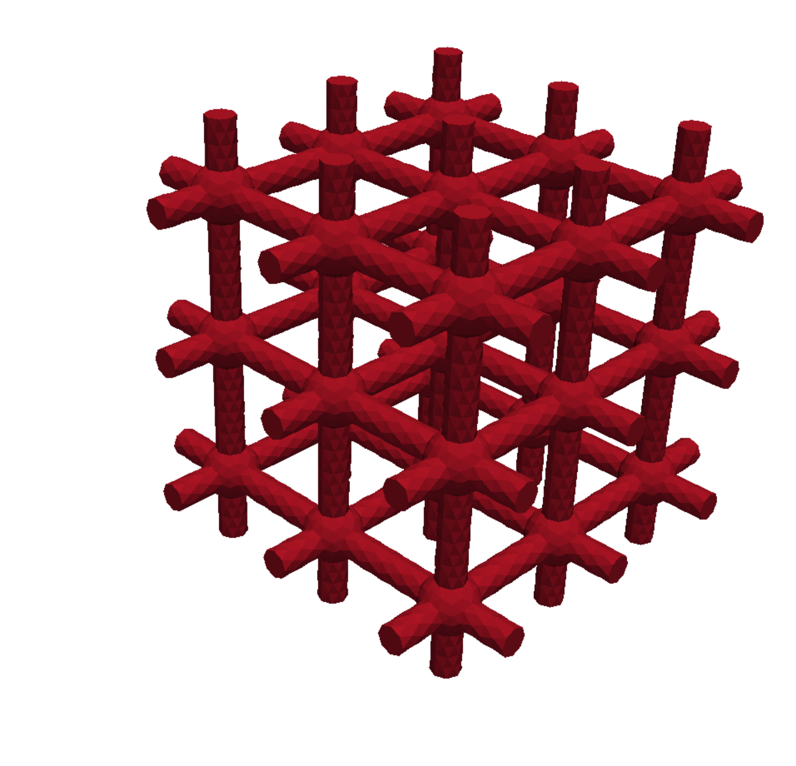
A reference cubic spline box is defined by a lattice of the control points P^i\hat{\textbf{{P}}}^{\,{\textbf{{i}}}} with ij∈{1,…,mj}i_{j}\in\{1,\ldots,m_{j}\}, where mjm_{j} is given by the spline order and the number of segments in the jj-th direction (see figure 1). The initial control points are placed at the Greville abscissae possibly resulting in a nonregular lattice.

Lattice periodicity is considered for all control points at the boundary of the spline box. We call an index i=(i1,i2,i3){\textbf{{i}}}=(i_{1},i_{2},i_{3}) with ik=1i_{k}=1 for at least one k∈{1,2,3}k\in\{1,2,3\} a master index labeled by iM{\textbf{{i}}}^{M} and an index with ik=mki_{k}=m_{k} for at least one k∈{1,2,3}k\in\{1,2,3\} a slave index labeled by iS{\textbf{{i}}}^{S}. Simply choosing 𝜶iS=𝜶iM{\mbox{\boldmath$\alpha$\unboldmath}}^{{\textbf{{i}}}^{S}}={\mbox{\boldmath$\alpha$\unboldmath}}^{{\textbf{{i}}}^{M}} would only permit for deformations where the eight outermost vertices still define a cube. To account for more flexible designs we add additional design variables 𝜷k∈ℝ3,k=1,2,3,{\mbox{\boldmath$\beta$\unboldmath}}_{k}\in{\mathbb{R}}^{3},k=1,2,3, and define

𝜷ki={𝜷k if ​ik=mk,0 else,{\mbox{\boldmath$\beta$\unboldmath}}^{\textbf{{i}}}_{k}=\begin{cases}{\mbox{\boldmath$\beta$\unboldmath}}_{k}&\text{ if }i_{k}=m_{k}\;,\\ 0&\text{ else}\;,\end{cases} (60)

and

𝜶i=𝜶~i+∑k=13𝜷ki.{\mbox{\boldmath$\alpha$\unboldmath}}^{\textbf{{i}}}=\tilde{\mbox{\boldmath$\alpha$\unboldmath}}^{\textbf{{i}}}+\sum_{k=1}^{3}{\mbox{\boldmath$\beta$\unboldmath}}^{\textbf{{i}}}_{k}\;. (61)

Thus, each 𝜷k{\mbox{\boldmath$\beta$\unboldmath}}_{k} translates one (slave) face of the lattice without deforming it allowing for sheared boxes as well. The lattice periodicity is then established by

PiS=𝒫#​PiM,{\textbf{{P}}}^{{\textbf{{i}}}^{S}}=\mathcal{P}_{\#}{\textbf{{P}}}^{{\textbf{{i}}}^{M}}\;, (62)

where 𝒫#\mathcal{P}_{\#} ensures 𝜶~iS=𝜶~iM\tilde{\mbox{\boldmath$\alpha$\unboldmath}}^{{\textbf{{i}}}^{S}}=\tilde{\mbox{\boldmath$\alpha$\unboldmath}}^{{\textbf{{i}}}^{M}}.

Figure 1: A spline box for mj=4,j=1,2,3,m_{j}=4,j=1,2,3, resulting in 64 control points.

For the two-scale setting we also want to allow for rotation of the microscopic unit cell. We introduce additional parameters 𝜽∈[0;π2]3{\mbox{\boldmath$\theta$\unboldmath}}\in[0;\tfrac{\pi}{2}]^{3} for rotation around the three coordinate axes. However, we do not rotate the spline box directly but rather the homogenized coefficients by

I​Hr=R​(𝜽)​I​H​R​(𝜽)⊤,{{\rm I}\kern-1.99997pt{\rm H}}_{r}={\textbf{{R}}}({\mbox{\boldmath$\theta$\unboldmath}})\;{{\rm I}\kern-1.99997pt{\rm H}}\;{\textbf{{R}}}({\mbox{\boldmath$\theta$\unboldmath}})^{\top}, (63)

where R is a corresponding rotation matrix.

5.1 Regularity preserving injectivity conditions

As already mentioned in the introduction, we do not want to remesh or refine the initial finite element mesh in our numerical examples. Thus, we have to prevent the mesh from degeneration due to design changes and hence, we have to ensure injectivity of the mapping defined in (59). For this some notations as well as a few geometrical concepts are introduced. Let ik+=i+ek{\textbf{{i}}}_{k}^{+}={\textbf{{i}}}+e_{k} and ik−=i−ek{\textbf{{i}}}_{k}^{-}={\textbf{{i}}}-e_{k}, k=1,2,3k=1,2,3, where e1=(1,0,0),e2=(0,1,0),e3=(0,0,1)e_{1}=(1,0,0),e_{2}=(0,1,0),e_{3}=(0,0,1). For k∈{1,2,3}k\in\{1,2,3\} we define the index set

I(k)={i|ij=1,…,mj for j≠k and ik=1,…,mk−1}.I(k)=\{{\textbf{{i}}}\;|\;i_{j}=1,\ldots,m_{j}\text{ for }j\neq k\text{ and }i_{k}=1,\ldots,m_{k}-1\}\;. (64)

Following the approach in [26] we define for i∈I⁡(k){\textbf{{i}}}\in I(k) the finite differences

Δki=Pik+−Pi\Delta^{\textbf{{i}}}_{k}={\textbf{{P}}}^{{\textbf{{i}}}_{k}^{+}}-{\textbf{{P}}}^{{\textbf{{i}}}} (65)

of two adjacent control points. Then the first derivative of x in (59) with respect to tkt_{k} may be expressed as

δtk​x=∑i∈I⁡(k)ωi​Δki​ℬik−​(t),\delta_{t_{k}}{\textbf{{x}}}=\sum_{{\textbf{{i}}}\in I(k)}\omega^{\textbf{{i}}}\Delta^{\textbf{{i}}}_{k}\mathcal{B}^{{\textbf{{i}}}_{k}^{-}}({\textbf{{t}}})\;, (66)

where ωi\omega^{\textbf{{i}}} is a positive factor independent of the control points.

Definition 5.1.

Let the convex hull of a subset XX of a vector space VV be defined by

convX={∑i=1nλixi|xi∈X,n∈ℕ,∑i=1nλi=1,λi≥0}.\conv X=\left\{\sum_{i=1}^{n}\lambda_{i}x_{i}\;\big|\;x_{i}\in X,n\in\mathbb{N},\sum_{i=1}^{n}\lambda_{i}=1,\lambda_{i}\geq 0\right\}\;. (67)

The conical hull of a subset XX of a vector space VV is given by

coniX={∑i=1nλixi|xi∈X,n∈ℕ,λi≥0}.\coni X=\left\{\sum_{i=1}^{n}\lambda_{i}x_{i}\;\big|\;x_{i}\in X,n\in\mathbb{N},\lambda_{i}\geq 0\right\}\;. (68)

A subset XX of a vector space VV is called cone, if

x∈X,λ∈ℝ,λ≥0⇒λ​x∈X.x\in X,\lambda\in{\mathbb{R}},\lambda\geq 0\Rightarrow\lambda x\in X\;. (69)

Finally we denote by X∗X^{*} the blunt cone X∖{0}X\setminus\{0\}.

Note that by this definition each cone or conical hull contains the point of origin and a conical hull is always a convex cone.

Definition 5.2.

Two cones C1,C2C_{1},C_{2} are said to be transverse if C1∪−C1C_{1}\cup-C_{1} and C2∪−C2C_{2}\cup-C_{2} intersect only at {0}\{0\}. Three cones C1,C2,C3C_{1},C_{2},C_{3} are said to be cotransverse if the origin is a vertex of the convex hull of C1,C2,C3C_{1},C_{2},C_{3} and the cone CiC_{i} and the convex hull of the cones Cj,CkC_{j},C_{k} are transverse for all {i,j,k}={1,2,3}\{i,j,k\}=\{1,2,3\}.

We now define cones generated by the forward finite differences of adjacent control points in each direction kk by

Ck=coni⁡{Δki|i∈I⁡(k)}.C_{k}=\coni\{\Delta^{\textbf{{i}}}_{k}\;|\;{\textbf{{i}}}\in I(k)\}\;. (70)

Using the previous definitions we are able to claim the following statement.

Proposition 5.3.

Let the mapping (59) be at least C1C^{1} and the boundary surfaces for fixed 𝛂\alpha not intersect and have no self-intersection point. Let further

  • (A1)

    Δki≠0\Delta^{\textbf{{i}}}_{k}\neq 0 for all i,k{\textbf{{i}}},k and

  • (A2)

    the cones C1,C2,C3C_{1},C_{2},C_{3} be cotransverse.

Then the mapping is injective on [0,1]3[0,1]^{3}.

Proof.

See [26, Proposition 3.4]. ∎

Next we want to derive sufficient conditions for (A​1)(A1) and (A​2)(A2). As a consequence of (A​2)(A2) the blunt cones Ck∗​(k=1,2,3)C_{k}^{*}(k=1,2,3) are pairwise disjoint. As the cones CkC_{k} are also convex, we can conclude by the hyperplane separation theorem that there exist three planes separating the blunt cones Ck∗C_{k}^{*} from each other. By the same argument we deduce the existence of planes separating one blunt cone from the convex hull of the other two. This also holds for the mirrored cones −Ck∗-C_{k}^{*} with the same planes as the separated sets just switch sides or signs in the formula, respectively.

To obtain sufficient conditions we first define four planes

H1​(x)=x1−x2−x3,H2​(x)=x1−x2+x3,H3​(x)=x1+x2−x3,H4​(x)=x1+x2+x3,\begin{split}H_{1}({\textbf{{x}}})=x_{1}-x_{2}-x_{3}\;,\quad&H_{2}({\textbf{{x}}})=x_{1}-x_{2}+x_{3}\;,\\ H_{3}({\textbf{{x}}})=x_{1}+x_{2}-x_{3}\;,\quad&H_{4}({\textbf{{x}}})=x_{1}+x_{2}+x_{3}\;,\end{split} (71)

and cones

C10={x∈ℝ3:H1(x)>0,H2(x)>0,H3(x)>0,H4(x)>0}∪{0},C20={x∈ℝ3:H1​(x)​<0,H2​(x)​<0,H3​(x)>​0,H4​(x)>​0}∪{0},C30={x∈ℝ3:H1(x)<0,H2(x)>0,H3(x)<0,H4(x)>0}∪{0},\begin{split}C_{1}^{0}&=\left\{{\textbf{{x}}}\in{\mathbb{R}}^{3}:H_{1}({\textbf{{x}}})>0,H_{2}({\textbf{{x}}})>0,H_{3}({\textbf{{x}}})>0,H_{4}({\textbf{{x}}})>0\right\}\cup\{0\}\,,\\ C_{2}^{0}&=\left\{{\textbf{{x}}}\in{\mathbb{R}}^{3}:H_{1}({\textbf{{x}}})<0,H_{2}({\textbf{{x}}})<0,H_{3}({\textbf{{x}}})>0,H_{4}({\textbf{{x}}})>0\right\}\cup\{0\}\,,\\ C_{3}^{0}&=\left\{{\textbf{{x}}}\in{\mathbb{R}}^{3}:H_{1}({\textbf{{x}}})<0,H_{2}({\textbf{{x}}})>0,H_{3}({\textbf{{x}}})<0,H_{4}({\textbf{{x}}})>0\right\}\cup\{0\}\,,\end{split} (72)

see also figure 2.

Figure 2: left: the cotransverse cones C10C_{1}^{0} (blue), C20C_{2}^{0} (red) and C30C_{3}^{0} (green). right: the regularized cones with parameter δ\delta.
Lemma 5.4.

The cones C10,C20,C30C_{1}^{0},C_{2}^{0},C_{3}^{0} are cotransverse.

Proof.

It is easy to see that the origin is a vertex of the convex hull of the cones

conv{C10,C20,C30}={x∈ℝ3:H1(x)≠0,H2(x)≠0,H3(x)≠0,H4(x)>0}∪{0}.\begin{split}\conv\{C_{1}^{0},\>&C_{2}^{0},C_{3}^{0}\}=\\ &\left\{{\textbf{{x}}}\in{\mathbb{R}}^{3}:H_{1}({\textbf{{x}}})\neq 0,H_{2}({\textbf{{x}}})\neq 0,H_{3}({\textbf{{x}}})\neq 0,H_{4}({\textbf{{x}}})>0\right\}\cup\{0\}\;.\end{split}

Now, without loss of generality let i=1i=1. Let further

S:=conv⁡{C20,C30}={x∈ℝ3:H1(x)<0,H2(x)≠0,H3(x)≠0,H4(x)>0}∪{0}.\begin{split}S:=&\conv\{C_{2}^{0},C_{3}^{0}\}\\ =&\left\{{\textbf{{x}}}\in{\mathbb{R}}^{3}:H_{1}({\textbf{{x}}})<0,H_{2}({\textbf{{x}}})\neq 0,H_{3}({\textbf{{x}}})\neq 0,H_{4}({\textbf{{x}}})>0\right\}\cup\{0\}\;.\end{split}

Then (C10∪−C10)∩(S∪−S)={0}(C_{1}^{0}\cup-C_{1}^{0})\cap(S\cup-S)=\{0\} and thus C10C_{1}^{0} and SS are transverse. For i∈{2,3}i\in\{2,3\} we get a similar result and hence C10,C20,C30C_{1}^{0},C_{2}^{0},C_{3}^{0} are cotransverse. ∎

Then obviously the cones C1,C2,C3C_{1},C_{2},C_{3} defined by (72) are cotransverse if

Ck⊂Ck0,k=1,2,3.C_{k}\subset C_{k}^{0},\ k=1,2,3\;. (73)
Lemma 5.5.

C1,C2,C3C_{1},C_{2},C_{3} are cotransverse if

conv{Δki|i∈I(k)}⊂Ck0,k=1,2,3.\conv\{\Delta^{\textbf{{i}}}_{k}\;|\;{\textbf{{i}}}\in I(k)\}\subset C_{k}^{0},\ k=1,2,3\;. (74)
Proof.

For i∈I⁡(k){\textbf{{i}}}\in I(k) and k∈{1,2,3}k\in\{1,2,3\} we have

Ck=coni⁡{Δki|i∈I⁡(k)}=coni⁡conv⁡{Δki|i∈I⁡(k)}⊂coni⁡Ck0=Ck0,C_{k}=\coni\{\Delta^{\textbf{{i}}}_{k}\;|\;{\textbf{{i}}}\in I(k)\}=\coni\conv\{\Delta^{\textbf{{i}}}_{k}\;|\;{\textbf{{i}}}\in I(k)\}\subset\coni C_{k}^{0}=C_{k}^{0}\;,

i. e. (73) holds. ∎

We note that conditions (73) are sufficient but not necessary for (A​2)(A2) to hold. For example they forbid rotations of the initial spline box whereas the cones still would be cotransverse. However they can be realized by linear inequalities which we will see later on. The latter are not only easy to handle in an optimization algorithm but also there exist algorithms assuring strict feasibility during the optimization procedure up to a certain tolerance. But still the constraint (74) cannot be treated by standard optimization software directly as the cones Ck0C_{k}^{0} (k=1,2,3)(k=1,2,3) are not closed. As a remedy we introduce a regularization parameter δ>0\delta>0 and define

C1δ={x∈ℝ3:H1(x)≥δ,H2(x)≥δ,H3(x)≥δ,H4(x)≥δ},C2δ={x∈ℝ3:H1(x)≤−δ,H2(x)≤−δ,H3(x)≥δ,H4(x)≥δ},C3δ={x∈ℝ3:H1(x)≤−δ,H2(x)≥δ,H3(x)≤−δ,H4(x)≥δ}.\begin{split}C_{1}^{\delta}&=\left\{{\textbf{{x}}}\in{\mathbb{R}}^{3}:H_{1}({\textbf{{x}}})\geq\phantom{-}\delta,H_{2}({\textbf{{x}}})\geq\phantom{-}\delta,H_{3}({\textbf{{x}}})\geq\phantom{-}\delta,H_{4}({\textbf{{x}}})\geq\delta\right\}\,,\\ C_{2}^{\delta}&=\left\{{\textbf{{x}}}\in{\mathbb{R}}^{3}:H_{1}({\textbf{{x}}})\leq-\delta,H_{2}({\textbf{{x}}})\leq-\delta,H_{3}({\textbf{{x}}})\geq\phantom{-}\delta,H_{4}({\textbf{{x}}})\geq\delta\right\}\,,\\ C_{3}^{\delta}&=\left\{{\textbf{{x}}}\in{\mathbb{R}}^{3}:H_{1}({\textbf{{x}}})\leq-\delta,H_{2}({\textbf{{x}}})\geq\phantom{-}\delta,H_{3}({\textbf{{x}}})\leq-\delta,H_{4}({\textbf{{x}}})\geq\delta\right\}\,.\end{split} (75)
Corollary 5.6.

If conv⁡{Δki|i∈I⁡(k)}⊆Ckδ\conv\{\Delta^{\textbf{{i}}}_{k}\;|\;{\textbf{{i}}}\in I(k)\}\subseteq C_{k}^{\delta}, k=1,2,3k=1,2,3, then (A​1)(A1) and (A​2)(A2) hold.

This follows easily from Ckδ⊂Ck0C_{k}^{\delta}\subset C_{k}^{0} and 0∉Ckδ0\notin C_{k}^{\delta}. The relaxation parameter δ\delta shifts the cones C10,C20,C30C_{1}^{0},C_{2}^{0},C_{3}^{0} away from the point of origin (see figure 2).

Remark 3.

Due to the performed numerical experiments, we observe that during the optimization process, the finite element mesh is less prone to its degeneration with increasing δ\delta. It can be shown that δ\delta gives direct control over the minimal distance of two adjacent control points. Owing to the continuity of the map from the control points onto the finite element nodes (59), there is also a control over the maximal deformation of a finite element. However, a quantitative result remains to be shown.

Now we state the linear constraints derived from (73). For Δki∈Ck\Delta^{\textbf{{i}}}_{k}\in C_{k} with k=1,2,3k=1,2,3 and i∈I⁡(k){\textbf{{i}}}\in I(k) we have four inequalities of type

μs,k​Hs​(Δki)≥δ,\mu_{s,k}H_{s}(\Delta^{\textbf{{i}}}_{k})\geq\delta\;, (76)

where μs,k∈{−1;1}\mu_{s,k}\in\{-1;1\} is chosen appropriatly to match the inequality to one of those in the definition of CkδC_{k}^{\delta} (75). Recalling definition (65) and (59)2(\ref{eq-spl1})_{2}

Δki=Pik+−Pi,Pi​(𝜶i)=P^i+𝜶i\begin{split}\Delta^{\textbf{{i}}}_{k}={\textbf{{P}}}^{{\textbf{{i}}}_{k}^{+}}-{\textbf{{P}}}^{{\textbf{{i}}}}\;,\\ {\textbf{{P}}}^{\,{\textbf{{i}}}}({\mbox{\boldmath$\alpha$\unboldmath}}^{\textbf{{i}}})=\hat{\textbf{{P}}}^{\,{\textbf{{i}}}}+{\mbox{\boldmath$\alpha$\unboldmath}}^{\textbf{{i}}}\end{split}

and exploiting the linearity of HsH_{s} we finally get linear constraints for the design variables 𝜶\alpha of form

−μs,k​Hs​(αik+−αi)≤μs,k​Hs​(P^ik+−P^i)−δ.-\mu_{s,k}H_{s}(\alpha^{{\textbf{{i}}}_{k}^{+}}-\alpha^{\textbf{{i}}})\leq\mu_{s,k}H_{s}(\hat{\textbf{{P}}}^{{\textbf{{i}}}_{k}^{+}}-\hat{\textbf{{P}}}^{\,{\textbf{{i}}}})-\delta\;. (77)

These conditions are sufficient for injectivity of (59) for all deformations 𝜶\alpha. Hence applying them in the optimization problems described in the following sections we are able to prevent degeneration of the unit cell YY in each iteration of the optimization algorithm.

Remark 4.

We note that the choice of the planes HsH_{s} may strongly influence optimal solutions. Thus it might be better to choose them in a more problem specific way, for example widen cones and narrow others in exchange.

6 Numerical results

In this section, we present numerical examples illustrating the two kinds of optimization problems introduced in Sections 3.1 and 3.2. For both we consider the same initial design on the porous microstructure. With reference to the representative cell YY split according to (1), the pore YcY_{c} consists of 3 perpendicular cylindrical channels YciY_{c}^{i}, i=1,2,3i=1,2,3 forming a rectangular cross. At the intersection the channel axes, a sphere Yc4Y_{c}^{4} is placed, so that the periodic porosity is generated by Yc=⋃i=1,…,4YciY_{c}=\bigcup_{i=1,\dots,4}Y_{c}^{i}.

problem fig. rr κ0\kappa_{0} κ1\kappa_{1} s0s_{0} s1s_{1} #iter. objective rel. gain
S/P 4 0 2e-5 −∞-\infty - - 101 1.149 7.3%
S/P-bis 5 1 2e-5 −∞-\infty - - 35 1.082 1.0%
S/PX 7 0 −∞-\infty 2e-5 - - 159 1.192 11%
P/SX’ 8 0 - - 0.9 0.95 114 12.43e-5 330%
C/S 9 0 - - Φe​(A​A0)\Phi_{\textbf{{e}}}({{\rm A}\kern-6.00006pt{\rm A}}_{0}) - 41 4.298 2.2%
Table 1: The numerical examples for material optimization. For the problem definitions including explanations for the parameters r,κ0,κ1,s0,s1r,\kappa_{0},\kappa_{1},s_{0},s_{1} see section 3.1.

We apply a cubic spline box with three segments of degree three in each direction resulting in 216 control points (cf. figure 3) to parameterize the shape of YcY_{c}, noting that also the shape of YY can be modified within the periodicity constraints, as discussed in Section 5. Thus, after elimination of degrees of freedom by periodic boundary conditions, the free coordinates of the control points {𝜶i}\{{\mbox{\boldmath$\alpha$\unboldmath}}^{i}\} yield 375 design variables.

Refer to caption
Refer to caption
Figure 3: Left: The initial setup: a solid cube (blue) with three channels (red) intersecting at a hollow sphere (red). The spline box has three segments of degree three in each direction resulting in 216 control points with the control polygon shown in white. right: 3x3x3 repeated channel part

6.1 Material optimization

For k=1,2,3k=1,2,3 we choose gk=ek{\textbf{{g}}}^{k}=e_{k} unit vectors and ek{\textbf{{e}}}^{k} and 𝝈k{\mbox{\boldmath$\sigma$\unboldmath}}^{k} such that for the initial design Φek​(A​A)=A​Ak​k​k​k\Phi_{\textbf{{e}}}^{k}({{\rm A}\kern-6.00006pt{\rm A}})={{\rm A}\kern-6.00006pt{\rm A}}_{kkkk} and Φ𝝈k​(C​C)=C​Ck​k​k​k\Phi_{\mbox{\boldmath$\sigma$\unboldmath}}^{k}({{\rm C}\kern-6.00006pt{\rm C}})={{\rm C}\kern-6.00006pt{\rm C}}_{kkkk}. The stiffness of the initial design is Φek​(A​A)=1.071\Phi_{\textbf{{e}}}^{k}({{\rm A}\kern-6.00006pt{\rm A}})=1.071 or Φ𝝈k​(C​C)=4.206\Phi_{\mbox{\boldmath$\sigma$\unboldmath}}^{k}({{\rm C}\kern-6.00006pt{\rm C}})=4.206, respectively, and the permeability is Ψk​(K)=4.3⋅10−5\Psi^{k}({\textbf{{K}}})=4.3\cdot 10^{-5} in each direction k=1,2,3k=1,2,3.

For the optimization we set the bounds for the directional permeabilities κ0=2⋅10−5\kappa_{0}=2\cdot 10^{-5}, and also the geometry regularization parameter introduced in (77), δ=0.02\delta=0.02. We solve the optimization problems using the sparse nonlinear optimizer SNOPT. In contrast to Fig. 3, we omit visualization of the control polygon in all forthcoming figures.

For problems S/P, S/P-bis, S/PX we choose γk=13,k=1,2,3\gamma^{k}=\tfrac{1}{3},k=1,2,3. The achieved solution of problem S/P is shown in Fig. 4. The optimized design follows our intuition how to maximize the stiffness; diamteres of the channels in all the three directions and the sphere are made as small as possible, thus, allowing for increasing the skeleton stiffness. The channels still form a rectangular cross, since no direction is preferred. The achieved stiffness is Φe​(A​A)=1.149\Phi_{\textbf{{e}}}({{\rm A}\kern-6.00006pt{\rm A}})=1.149, i.e. improvement by 7.3%7.3\%, whereby the permeability constraints are all active at their lower bounds.

Refer to caption
Refer to caption
Figure 4: Left: The optimized unit cell geometry regarding Problem S/P. The objective was improved by 7.3%7.3\%. right: 3x3x3 repeated channel part

For problem S/P-bis, the resulting optimized microstructure is displayed in Fig. 5. In consequence of the considered volume preservation of YcY_{c}, the channels get wider near to the boundary of the unit cell. In fact the diameter of the channels is approximately equal to the diameter of the deformed sphere. Also in this case the optimized redistribution of the solid material has a rather intuitive explanation – since the channel junction is the weakest area in the cell YY, therefore, the pore volume is reduced as much as possible (by virtue of the channels diameters) within the other design constraints. The stiffness of the optimized microstructure improved by 1.0%1.0\% only, attaining Φe​(A​A)=1.082\Phi_{\textbf{{e}}}({{\rm A}\kern-6.00006pt{\rm A}})=1.082, The permeability constraint for k=3k=3, and the volume constraint are active, however, permeability constraints Ψk​(K)=2.9⋅10−5\Psi^{k}({\textbf{{K}}})=2.9\cdot 10^{-5} for k=1,2k=1,2 are nonactive, which corresponds to the nonsymmetric design. It should be noted at this point, that the deformation of the boundary of the unit cell is due to numerical reasons but only has little influence on the resulting design, as the cell is considered to be repeated periodically.

Refer to caption
Refer to caption
Figure 5: The optimization result of problem S/P-bis. The stiffness was improved by 1.0%1.0\%. Note the widening of the channels at the boundaries due to the forced volume preservation of the channel part.
Figure 6: Convergence plots for problems S/P-bis (left) and P/SX (right)

In all the previous examples the bounds on the permeability constraints along the principal axes gk{\textbf{{g}}}^{k} as well as the weights γk\gamma^{k} in the objective function Φe\Phi_{\textbf{{e}}} were chosen completely symmetric enforcing almost isotropic designs. For problem S/PX, see (13), we set β1=β2=49,β3=19\beta^{1}=\beta^{2}=\tfrac{4}{9},\beta^{3}=\tfrac{1}{9} and κ1=2⋅10−5\kappa_{1}=2\cdot 10^{-5}. Due to the different weights of the directional permeabilities, the optimization results in a remarkably anisotropic design, as can be seen in Fig. 7. The permeability in the first direction is more important than the one in the third direction, thus the channel in the first direction is much wider than the one in the third direction. Also a wider channel would be needed to increase the permeability in the second direction. However, this is not possible because of to the chosen design parametrization.

Refer to caption
Refer to caption
Figure 7: The optimized geometry for problem S/PX. The stiffness was improved by 11%11\%.

An optimization result of problem P/SX’, see (14), is shown in Fig. 8. We choose βk=13,k=1,2,3\beta^{k}=\tfrac{1}{3},k=1,2,3 as weights for the permeability sum, s0=0.9s_{0}=0.9 and s1=0.95s_{1}=0.95 together with the weights for the stiffness sum γ1=813,γ2=413,γ3=113\gamma^{1}=\tfrac{8}{13},\gamma^{2}=\tfrac{4}{13},\gamma^{3}=\tfrac{1}{13}. The choice s0≈s1s_{0}\approx s_{1} leads to almost symmetric design of the microstructure, although the stiffnesses in the preferred directions reflect the decreasing sequence of γk\gamma^{k}, k=1,2,3k=1,2,3, namely Φe1​(A​A)=0.96,Φe2​(A​A)=0.94,Φe3​(A​A)=0.90\Phi_{\textbf{{e}}}^{1}({{\rm A}\kern-6.00006pt{\rm A}})=0.96,\Phi_{\textbf{{e}}}^{2}({{\rm A}\kern-6.00006pt{\rm A}})=0.94,\Phi_{\textbf{{e}}}^{3}({{\rm A}\kern-6.00006pt{\rm A}})=0.90. Also in this case, to increase the stiffness in direction e1{\textbf{{e}}}^{1}, the sphere in the middle is stretched in this direction. The achieved objective function value is Ψ⁡(K)=12.4⋅10−5\Psi({\textbf{{K}}})=12.4\cdot 10^{-5} gives rise to an improvement by 328%328\% with respect to the initial design.

Refer to caption
Refer to caption
Figure 8: The optimization result of problem P/SX’. The permeability was improved by 328%328\%.

To solve the minimization problem C/S, see (16), we set s0=Φe​(A​A0)s_{0}=\Phi_{\textbf{{e}}}({{\rm A}\kern-6.00006pt{\rm A}}_{0}), where A​A0{{\rm A}\kern-6.00006pt{\rm A}}_{0} is the stiffness tensor of the drained initial design again with γk=13,k=1,2,3\gamma^{k}=\tfrac{1}{3},k=1,2,3. In this case, since the porous material permeability is irrelevant, the undrained stiffness maximization induces redistribution of the solid phase so that the sphere in the middle of the cell YY is blown up whilst the channels are getting rather smaller near to the (periodic) boundary ∂Y\partial Y, see Fig. 9. This shape modification reflects the trend to create one spherical inclusion; note that the drained stiffnesses (as measured in directions k=1,2,3k=1,2,3) is bounded due to the imposed constraints. Compared to the initial layout, the undrained compliance, i.e. the objective, decreased merely by 2.1%2.1\%.

Refer to caption
Refer to caption
Figure 9: The optimized geometry for problem C/S. The objective (the undrained stiffness) was improved by 2.1%2.1\%.

6.2 Numerical illustrations for the 2-scale optimization

Next we present numerical solutions of problem (31) at a location of interest defined in a given macroscopic domain. First we solve the macroscopic problems (17) and (18) on a cuboid domain discretized by 15x10x2 finite elements, see Fig. 10, where the geometry of the macroscopic specimen (domain Ω\Omega) and the boundary conditions are depicted. On a part of ΓN\Gamma_{N}, surface stresses are applied, while the body is fixed at ΓD\Gamma_{D}. We prescribe pressure at Γp1\Gamma_{p}^{1} by p¯1=1\bar{p}^{1}=1 and at Γp2\Gamma_{p}^{2} by p¯2=0.5\bar{p}^{2}=0.5. Problem (31) also involves the Lagrange multiplier Λ\Lambda which is a priori unknown. Thus, we consider different values of Λ\Lambda for which the adjoint system (37) must be solved. From the definition of the macroscopic problem in (23), it is readily seen that a positive Λ>0\Lambda>0 means too much fluid flows through Γp2\Gamma_{p}^{2}, while a negative Λ<0\Lambda<0 means the opposite, the flow is insufficient. The solution of the state problems is displayed in Fig. 10, while solutions of the adjoint system for Λ=−1\Lambda=-1 and Λ=1\Lambda=1 can be seen in Fig. 11.

Refer to caption
Refer to caption
Figure 10: Left: The setup of the macroscopic domain for the 2-scale examples. On a portion of boundary ΓN\Gamma_{N} marked by “f”, the body is loaded by traction forces. Right: The solution of the state problem (front view). The color encodes magnitude of pressure pp and the arrows show directions and magnitudes of the fluid velocity.
Refer to caption
Refer to caption
Figure 11: Left: The adjoint solution for Λ=−1\Lambda=-1. Right: The adjoint solution for Λ=1\Lambda=1. The color encodes magnitude of q~\tilde{q} and the arrows show direction and magnitude of v~\tilde{v}. Note the opposite flow direction in the highlighted area next to Γp2\Gamma_{p}^{2} which is a consequence of the sign of the multiplier Λ\Lambda.

We select one finite element A located next to Γp1\Gamma_{p}^{1} for which the locally periodic microstructure is optimized by virtue of the local nonlinear optimization problem (31). The same initial structure for the microscopic cell YY is considered as in section 6, whereby the design variables are associated with the control points of a cubic spline box with three segments in each direction. In addition, by virtue of (63), we allow for a reorientation of the cell YY due to the rotation around the third axis.

For the selected finite element, the macroscopic tensors (32) are computed as the average evaluated using the values at the Gauss points. The main eigenvector of (∇P⊗∇q~)−Λ⁡(∇P⊗∇p~)(\nabla P\otimes\nabla\tilde{q})-\Lambda(\nabla P\otimes\nabla\tilde{p}) corresponds to the fluid velocity vector and points into direction w=[0.22,−0.97,0]{\textbf{{w}}}=[0.22,-0.97,0]. If we interpret (e​(u)⊗e​(v~))({\textbf{{e}}}({{\textbf{{u}}}})\otimes{\textbf{{e}}}({\tilde{\textbf{{v}}}})) as a fourth-order stiffness tensor, then the direction of the main stiffness points approximately into direction s=[1,0,0]{\textbf{{s}}}=[1,0,0]. Thus, we expect the microscopic result to have the highest permeability in direction w and highest stiffness in direction s. However, if we look at the convergence plot in Fig. 13 we observe that the first term clearly dominates the objective function values. As a result, the terms involving the permeability are neglected by the optimizer which focuses on increasing the stiffness of the microscopic structure in direction s. This leads to a minimization of the channel part lumen in each cross section of YY perpendicular to s (cf. fig. 12).

Refer to caption
Refer to caption
Figure 12: The optimized unit cell geometry for Λ=−1\Lambda=-1. The structure is rotated by α=0.022∘\alpha=0.022^{\circ} around the third axis.
Figure 13: Convergence plot for the 2-scale problem in finite element A with Λ=−1\Lambda=-1.

If we choose Λ=−100\Lambda=-100, still the stiffness term has most influence on the objective function, as can be seen in Fig. 15. However, the importance of the permeability terms increases. The optimized structure seen in Fig. 14 is featured by a wide channel in vertical direction rotated by 66 degrees, which is half the angle between w and the second axis. This time the stiffness tensor is almost isotropic, with only 3%3\% difference between the largest and smallest directional stiffness. Owing to this, the rotation of the unit cell has negligible influence on the first term of the objective. Thus a rotation is chosen which increases the permeability in direction w and hence the overall objective.

Refer to caption
Refer to caption
Figure 14: The optimized geometry for Λ=−100\Lambda=-100. The structure is rotated by α=6.3∘\alpha=6.3^{\circ} around the third axis.
Figure 15: Convergence plot for the 2-scale problem in finite element A with Λ=−100\Lambda=-100.

As displayed in Fig. 16, the impact of the terms involving the permeability increases with decreasing Λ\Lambda. However, the optimized structure for Λ=−1000\Lambda=-1000 is quite similar the one obtained forΛ=−100\Lambda=-100, moreover, also the rotations are similar.

Figure 16: Convergence plot for Λ=−1000\Lambda=-1000

7 Conclusion and outlook

In this study we described a methodology to optimize porous material microstructures using the shape optimization approach. The optimality criteria are based on the effective poroelastic material coefficients. By virtue of homogenization, these coefficients are evaluated using the characteristic responses of the representative periodic cell YY. Sensitivities with respect to Biot coefficients as well as shape parameters were provided. The shape of the fluid-filled pores was parameterized using B-spline boxes combined with only mildly restrictive regularity constraints. As an advantage of the chosen spline parametrization, it provides automatically the so-called design velocity fields used in the sensitivity computations which are based on the material derivative approach. We considered optimization of the stiffness maximization subject to constraints related to the permeability and vice versa. While in a fully symmetric setup, only moderate improvements of the chosen cost functions were possible, in an anisotropic setup significant improvements could be obtained fully exploiting the given design freedom. These anisotropic layouts appear very naturally, when local microstructures are used to optimize some global macroscopic criterion of interest.

Following this idea, we considered a two-scale optimization problem related to the structure compliance minimization with constraints on the fluid transport. Using the sensitivity analysis described above, a local optimization problem was derived, which is essentially a linearization of the macroscopic problem with respect to the poroelastic coefficients involved in the Biot model. By virtue of the homogenization process, these coefficients themselves are parameterized by the underlying microstructure layout; in this study, the shape of the pores is described by the spline box, cf. [2] where the topology optimization approach was treated. Due to its separable character, this linearized problem of the locally optimal design can be solved cell by cell. As an example illustrating our approach, we discussed optimization results for particular areas of interest in the macroscopic domain. Our study should be considered as the first step towards a full two-scale optimization approach in the framework of which sequential linearizations of the given type may be used to solve the entire two-scale optimization problem. To develop a robust two-scale optimization tool providing optimized microstructure designs in a macroscopic domain, yet some technical issues will have to be treated, such as connectivity of the pores on the boundary between subdomains of locally optimized periodic designs.

There are several extensions of the present work which are of interest in the context of smart structures and the material design. In particular, including the piezoelectric components in the microstructure will enable to control and optimize the fluid redistribution in the porous structure by the electric field; in this context, homogenization of the poro-piezoelectric materials reported in [22] can serve a suitable framework. Another important extension of the present study is by including the inertia effects in the micromodel. This will allow for optimization of dynamic response of the porous structures to control the acoustic wave propagation and the wave dispersion.

Acknowledgment

This research was supported by project GACR 16-03823S and in part by projects GACR 13-00863S and LO 1506 of the Czech Ministry of Education, Youth and Sports, which enabled short visits of the first author in the NTIS, the University of West Bohemia in Pilsen.

References

  • [1] G. Allaire, Shape Optimization by the Homogenization Method, Springer, New York, 2001.
  • [2] C. S. Andreasen, O. Sigmund, Topology optimization of fluid–structure-interaction problems in poroelasticity. Comput. Methods Appl. Mech. Engrg. 258 (2013) 55–62.
  • [3] J. L. Auriault, E. Sanchez-Palencia, Étude du comportement macroscopique d’un milieu poreux sature deformable, Jour. de Mécanique 16 (4) (1977) 575–603.
  • [4] C. Barbarosie, A.-M. Toader, Shape and topology optimization for periodic problems, Struct Multidisc Optim 40 (2010) 381–391
  • [5] C. Barbarosie, A.-M. Toader, Optimization of bodies with locally periodic microstructure, Mechanics of advanced materials and structures, 19.4 (2012) 290–301.
  • [6] M. P. Bendsøe, O. Sigmund, Topology optimization: theory, methods, and applications. Springer-Verlag, Berlin and Heidelberg 2003.
  • [7] M. A. Biot, Theory of elasticity and consolidation for a porous anisotropic solid, J. Appl. Phys. 26 (2) (1955) 182–185.
  • [8] D. Brown, P. Popov, Y. Efendiev, On homogenization of stokes flow in slowly varying media with applications to fluid-structure interaction, Int. Jour. on Geomathematics 2 (2) (2011) 281–305.
  • [9] R. Burridge, J. B. Keller, Poroelasticity equations derived from microstructure, Acoust. Soc. Am. 70 (1981) 1140–1146.
  • [10] R. Cimrman, et al., SfePy home page, http://sfepy.org, software, finite element code and applications (2011).
  • [11] M. C. Delfour, J.-P. Zolésio, Shapes and Geometries, Advances in Design and Control, SIAM, 2011.
  • [12] J. K. Guest, J. H. Prévost, Optimizing multifunctional materials: Design of microstructures for maximized stiffness and fluid permeability. International Journal of Solids and Structures 43 (2006) 7028–7047.
  • [13] J. Haslinger, R. A. E. Mäkinen, Introduction to shape optimization, Advances in Design and Control, SIAM, 2003.
  • [14] B. Hassani, E. Hinton, A review of homogenization and topology optimization I - homogenization theory for media with periodic structure, Computers and Structures, 69.6 (1998) 707–717.
  • [15] E. J. Haug, K. Choi, V. Komkov, Design Sensitivity Analysis of Structural Systems, Academic Press, Orlando, 1986.
  • [16] U. Hornung, Homogenization and porous media, Springer, Berlin, 1997.
  • [17] O. Iliev, A. Mikelic, P. Popov, On upscaling certain flows in deformable porous media, SIAM, Multiscale Model. Simul. 7 (2008) 93–123.
  • [18] C. K. Lee, C. C. Mei, Re-examination of the equations of poroelasticity, Int. J. Eng. Sci. 35 (1997) 329–352.
  • [19] A. Mikelic, M. Wheeler, On the interface law between a deformable porous medium containing a viscous fluid and an elastic body, Math. Models Meth. Appl. Sci. 22 (2012) 1–32.
  • [20] E. Rohan, Sensitivity strategies in modelling heterogeneous media undergoing finite deformation, Math. and Computers in Simulation 61 (3-6) (2003) 261–270.
  • [21] E. Rohan, V. Lukeš, On modelling nonlinear phenomena in deforming heterogeneous media using homogenization and sensitivity analysis concepts. Applied Mathematics and Computation 267 (2015) 583–595.
  • [22] E. Rohan, V. Lukeš, R. Cimrman, Homogenization of the fluid-saturated piezoelectric porous metamaterials. In Proceedings of the VII Int. Conf. on Computational Methods for Coupled Problems in Science and Engineering, COUPLED PROBLEMS 2017, M. Papadrakakis, E. Onate and B. Schrefler (Eds), 2017.
  • [23] E. Rohan, S. Naili, T. Lemaire, Double porosity in fluid-saturated elastic media: deriving effective parameters by hierarchical homogenization of static problem. Continuum Mech. Thermodyn. 28 (2016) 1263–1293.
  • [24] E. Rohan, S. Shaw, J. Whiteman, Poro-viscoelasticity modelling based on upscaling quasistatic fluid-saturated solids, Computational Geosciences (2013) DOI:10.1007/s10596–013–9363–1.
  • [25] S. Xu, G. Cheng, Optimum material design of minimum structural compliance under seepage constraint. Struct Multidisc Optim (2010) 41:575–587
  • [26] G. Xu, B. Mourrain, R. Duvigneau, A. Galligo, Optimal analysis-aware parameterization of computational domain in 3D isogeometric analysis, Computer-Aided Design 45 (2013) 812–821.