跳到论文正文
W Papers独立论文阅读器 arXiv:1802.00533 论文正文 计算阅读时间 · 0%
引用这篇论文根据当前论文元数据生成,正式投稿前建议核对。


License: arXiv.org perpetual non-exclusive license
arXiv:1802.00533v7 [math.MG] 29 Jul 2019

Persistent Homology and
the Upper Box Dimension

Benjamin Schweinhart
Date: July 2019
Abstract.

We introduce a fractal dimension for a metric space defined in terms of the persistent homology of extremal subsets of that space. We exhibit hypotheses under which this dimension is comparable to the upper box dimension; in particular, the dimensions coincide for subsets of ℝ2\mathbb{R}^{2} whose upper box dimension exceeds 1.5.1.5. These results are related to extremal questions about the number of persistent homology intervals of a set of nn points in a metric space.

1. Introduction

Several notions of fractal dimensions based on persistent homology have been proposed in the literature, including in the PhD thesis of Vanessa Robins [25], in a paper written by Robert MacPherson and the current author [21], and by Adams et al. [1]. In that work, empirical estimates of the proposed dimensions were compared with classically defined fractal dimensions. Here, we prove the first rigorous analogue of those comparisons.

Refer to caption
Refer to caption
Refer to caption
Figure 1. Examples which satisfy the hypotheses of our main theorem: the Sierpinski triangle (dimbox=log⁡(3)/log⁡(2)≈1.585\text{dim}_{\text{box}}=\log\left(3\right)/\log\left(2\right)\approx 1.585), Schramm–Loewner Evolution with κ=6\kappa=6 (dimbox≥dimHausdorff=7/4\text{dim}_{\text{box}}\geq\text{dim}_{\text{Hausdorff}}=7/4 [2]), Figure provided by T. Kennedy [18]), and the Ikeda attractor (dimbox≈1.7\text{dim}_{\text{box}}\approx 1.7 assuming that computational estimates of the box dimension of that set accurate).

The motivation for the definition proposed here comes from the literature on minimal spanning trees. The properties of minimal spanning trees of point collections contained in a bounded subset of ℝm\mathbb{R}^{m} have long been of interest [28, 19]. In 2005, Kozma, Lotker, and Stupp [20] proved a relationship between the extremal behavior of these trees and the upper box dimension. To be precise, let T⁡(y)T\left(\textbf{y}\right) denote the minimal spanning tree of a finite metric space y and let

Eα0​(y)=12​∑e∈T⁡(Y)|e|α,E_{\alpha}^{0}\left(\textbf{y}\right)=\frac{1}{2}\sum_{e\in T\left(Y\right)}\left|e\right|^{\alpha}\,,

where the sum is taken over all edges ee in the tree T⁡(y),T\left(\textbf{y}\right), and |e|\left|e\right| denotes the length of the edge.

Definition 1.

If XX is a bounded metric space, let dimMST​(X)\text{dim}_{\text{MST}}\left(X\right) be the infimal exponent α\alpha so that Eα0​(x)E_{\alpha}^{0}\left(\textbf{x}\right) is uniformly bounded for all finite point sets x⊂X:\textbf{x}\subset X:

dimMST​(X)=inf{α:∃C​ so that ​Eα0​(x)<C​∀ finite ​x⊂X}.\text{dim}_{\text{MST}}\left(X\right)=\inf\left\{\alpha:\exists\,C\text{ so that }E_{\alpha}^{0}\left(\textbf{x}\right)<C\;\forall\text{ finite }\;\textbf{x}\subset X\right\}\,.

Kozma, Lotker, and Stupp proved that dimMST​(X)\text{dim}_{\text{MST}}\left(X\right) equals the upper box dimension [3] of X.X.

Definition 2.

Let XX be a bounded metric space and let Nδ​(X)N_{\delta}\left(X\right) be the maximal number of disjoint closed δ\delta-balls with centers in X.X. The upper box dimension of XX is

dimbox​(X)=lim supδ→0log⁡(Nδ​(X))log⁡(1/δ).\begin{split}\text{dim}_{\text{box}}\left(X\right)=\limsup_{\delta\rightarrow 0}{\frac{\log\left(N_{\delta}\left(X\right)\right)}{\log\left(1/\delta\right)}}\,.\end{split}
Theorem 3 (Kozma, Lotker, and Stupp [20]).

For any metric space X,X,

dimMST​(X)=dimbox​(X).\text{dim}_{\text{MST}}\left(X\right)=\text{dim}_{\text{box}}\left(X\right)\,.

If x is a finite point set contained in a bounded metric space, and 𝑃𝐻i​(x)\mathit{PH}_{i}\left(\textbf{x}\right) is the ii-dimensional persistent homology of the Čech complex of x,\textbf{x}, there is a bijection between the edges of the Euclidean minimal spanning tree of x and the intervals in the canonical decomposition of 𝑃𝐻0​(x),\mathit{PH}_{0}\left(\textbf{x}\right), where the length of an interval in 𝑃𝐻0​(x)\mathit{PH}_{0}\left(\textbf{x}\right) is half the length of the corresponding edge. (Note that if persistent homology is taken of the Rips complex of x,\textbf{x}, then a similar correspondence holds without the requirement of an ambient space, where an interval corresponds to the edge of the same length.) This observation suggests a generalization of the previous result to higher-dimensional persistent homology. Namely, let

Eαi​(x)=∑(b,d)∈𝑃𝐻i​(x)(d−b)αE_{\alpha}^{i}\left(\textbf{x}\right)=\sum_{\left(b,d\right)\in\mathit{PH}_{i}\left(\textbf{x}\right)}\left(d-b\right)^{\alpha}

where the sum is taken over all bounded 𝑃𝐻i\mathit{PH}_{i} intervals and define:

Definition 4.

Let XX be a bounded subset of a metric space. The 𝑃𝐻i\mathit{PH}_{i}-dimension of XX is

dim𝑃𝐻i​(X)=inf{α:∃C​ so that ​Eαi​(x)<C​∀ finite x⊂X}.\begin{split}\text{dim}_{\mathit{PH}}^{i}\left(X\right)=\inf\left\{\alpha:\exists\,C\text{ so that }E_{\alpha}^{i}\left(\textbf{x}\right)<C\;\forall\text{ finite }\textbf{x}\subset X\right\}\,.\end{split}

Also, let dim𝑃𝐻~i​(X)\text{dim}_{\widetilde{\mathit{PH}}}^{i}\left(X\right) be defined by replacing the Čech complex with the Rips complex in the previous construction.

Then

dim𝑃𝐻0​(X)=dim𝑃𝐻~0​(X)=dimMST​(X).\text{dim}_{\mathit{PH}}^{0}\left(X\right)=\text{dim}_{\widetilde{\mathit{PH}}}^{0}\left(X\right)=\text{dim}_{\text{MST}}\left(X\right)\,.

Note that dim𝑃𝐻~i​(X)\text{dim}_{\widetilde{\mathit{PH}}}^{i}\left(X\right) is defined for bounded metric spaces X,X, rather than bounded subsets of a metric space.

Question 5.

Are there hypotheses on XX under which dim𝑃𝐻i​(X)=dimbox​(X)\text{dim}_{\mathit{PH}}^{i}\left(X\right)=\text{dim}_{\text{box}}\left(X\right) or dim𝑃𝐻~i​(X)=dimbox​(X)\text{dim}_{\widetilde{\mathit{PH}}}^{i}\left(X\right)=\text{dim}_{\text{box}}\left(X\right) for i>0i>0?

Unlike the 0-dimensional case, equality will not always hold. For example, the 𝑃𝐻1\mathit{PH}_{1}-dimension of a line in ℝm\mathbb{R}^{m} will always be 0.0. Also, there are metric spaces not embeddable in any finite-dimensional Euclidean space whose 𝑃𝐻~1\widetilde{\mathit{PH}}_{1}-dimension exceeds their upper box dimension.

Proposition 6.

There is a metric space XX so that dim𝑃𝐻~1​(X)=2\text{dim}_{\widetilde{\mathit{PH}}_{1}}\left(X\right)=2 but dimbox​(X)=1.\text{dim}_{\text{box}}\left(X\right)=1.

We prove this in Section 5.1. This behavior is related to the existence of families of point sets {xn}n∈ℕ\left\{\textbf{x}_{n}\right\}_{n\in\mathbb{N}} for which number of intervals of 𝑃𝐻i​({xn})\mathit{PH}_{i}\left(\left\{\textbf{x}_{n}\right\}\right) grows slower or faster than linearly in in |xn|\left|\textbf{x}_{n}\right| when i>0i>0; by contrast, the reduced 00-dimensional persistent homology of a finite metric space with kk points always has k−1k-1 intervals.

We restrict our attention to subsets of Euclidean space, and conjecture

Conjecture 7.

For any m∈ℕm\in\mathbb{N} and 0≤i<m,0\leq i<m, there is a constant γim<m\gamma_{i}^{m}<m so that if X⊂ℝmX\subset\mathbb{R}^{m} and dimbox​(X)>γim\text{dim}_{\text{box}}\left(X\right)>\gamma_{i}^{m} then

dim𝑃𝐻i​(X)=dimbox​(X).\begin{split}\text{dim}_{\mathit{PH}}^{i}\left(X\right)=\text{dim}_{\text{box}}\left(X\right)\,.\end{split}

Cohen-Steiner, Edelsbrunner, Harer, and Mileyko studied a quantity similar to EαiE_{\alpha}^{i} in their paper [9]. Their results immediately imply that if X⊂ℝm,X\subset\mathbb{R}^{m}, then dim𝑃𝐻i(X)≤m\dim_{\mathit{PH}}^{i}\left(X\right)\leq m for all i∈ℕi\in\mathbb{N} (Corollary 15). If XX is a subset of ℝm\mathbb{R}^{m} with non-empty interior the corresponding lower bound is easy to show and dim𝑃𝐻i(X)=m\dim_{\mathit{PH}}^{i}\left(X\right)=m for i=1,…,m−1i=1,\ldots,m-1 ( Proposition 21). However, our focus here will be to prove results about subsets of fractional box dimension. This task is challenging, and involves difficult combinatorial problems. Our main result is:

Theorem 8.

Let XX be a bounded subset of ℝ2.\mathbb{R}^{2}. If dimbox​(X)>1.5,\text{dim}_{\text{box}}\left(X\right)>1.5, then

dim𝑃𝐻1​(X)=dimbox​(X).\begin{split}\text{dim}_{\mathit{PH}}^{1}\left(X\right)=\text{dim}_{\text{box}}\left(X\right)\,.\end{split}

See Figure 1 for images of two examples known to meet these hypotheses, and one that is believed to based on computational experiments. The upper bound dim𝑃𝐻1​(X)≤dimbox​(X)\text{dim}_{\mathit{PH}}^{1}\left(X\right)\leq\text{dim}_{\text{box}}\left(X\right) is proven in Section 3, and the lower bound in Section 4.

We also prove partial results in more general cases:

Theorem 9.

Let XX be a bounded subset of ℝm.\mathbb{R}^{m}. If dimbox​(X)>m−1/2,\text{dim}_{\text{box}}\left(X\right)>m-1/2, then

dimbox​(X)≤dim𝑃𝐻1​(X)≤m.\begin{split}\text{dim}_{\text{box}}\left(X\right)\leq\text{dim}_{\mathit{PH}}^{1}\left(X\right)\leq m\,.\end{split}

Furthermore, we show that the example in Proposition 6 cannot be taken to be a subset of ℝm.\mathbb{R}^{m}.

Theorem 10.

If XX is a bounded subset of ℝm\mathbb{R}^{m} then

dim𝑃𝐻~1​(X)≤dimbox​(X).\begin{split}\text{dim}_{\widetilde{\mathit{PH}}}^{1}\left(X\right)\leq\text{dim}_{\text{box}}\left(X\right)\,.\end{split}

In the process of proving this, we also show:

Theorem 11.

If x is a finite subset of ℝm\mathbb{R}^{m} then the first-dimensional persistent homology of the Rips complex of x contains O⁡(|x|)O\left(\left|\textbf{x}\right|\right) intervals.

In previous work with MacPherson [21], we defined an alternate notion of persistent homology dimension that measures the complexity of a shape rather than a classical notion of fractal dimension. In Appendix A, we show that it is a lower bound for dim𝑃𝐻1.\text{dim}_{\mathit{PH}}^{1}.

We prove the upper bounds for Theorems 8 and 9 in Section 3, and the lower bounds in Section 4. The results and arguments will be stated for the Čech complex, but we will indicate which ones also work for the Rips complex. We prove our results specific to the Rips complex in Section 5. First, we cover some preliminaries.

2. Preliminaries

In the introduction we defined the upper box dimension in terms of Nδ​(X),N_{\delta}\left(X\right), maximal number of disjoint closed balls centered at points of a bounded metric space X:X:

dimbox​(X)=lim supδ→0log⁡(Nδ​(X))log⁡(1/δ).\begin{split}\text{dim}_{\text{box}}\left(X\right)=\limsup_{\delta\rightarrow 0}{\frac{\log\left(N_{\delta}\left(X\right)\right)}{\log\left(1/\delta\right)}}\,.\end{split}

Note that this is equivalent to taking dimbox​(X)\text{dim}_{\text{box}}\left(X\right) to be the unique real number dd so that

  • •

    Nδ​(X)=O⁡(δ−α)N_{\delta}\left(X\right)=O\left(\delta^{-\alpha}\right) for all α>d.\alpha>d. That is, for all α>d\alpha>d there exists a C>0C>0 so that Nδ​(X)<C​δ−αN_{\delta}\left(X\right)<C\delta^{-\alpha} for all δ>0.\delta>0.

  • •

    Nδ​(X)≠O⁡(δ−α)N_{\delta}\left(X\right)\neq O\left(\delta^{-\alpha}\right) for all α<d.\alpha<d. That is, for all α<d\alpha<d and all D>0D>0 there exists a sequence δj→0\delta_{j}\rightarrow 0 so that Nδ​(X)>D​δ−αN_{\delta}\left(X\right)>D\delta^{-\alpha} for all j.j.

There are other equivalent definitions. In particular Nδ⁡(X)N_{\delta\left(X\right)} can be replaced by the minimum number of balls of radius δ\delta required to cover XX or, if X⊂ℝm,X\subset\mathbb{R}^{m}, the number of cubes in a regular square tesselation of ℝm\mathbb{R}^{m} of width δ\delta which intersect X.X. See Falconer [15] for details.

Also, if Δ\Delta is an kk-dimensional simplex in ℝm\mathbb{R}^{m}, the circumsphere of Δ\Delta is the smallest m−1m-1-dimesional sphere containing the vertices of Δ.\Delta. The circumradius of Δ\Delta is the radius of its circumsphere.

In the following, bold lower case letters will denote finite point sets (i.e. x,y\textbf{x},\textbf{y}) .

2.1. Persistent Homology

Here, we provide a brief introduction to persistent homology. For a more thorough exposition, see see [14, 12, 4]. We assume the reader is familiar with the basics of simplicial homology, as in [17].

2.1.1. Filtrations

Refer to caption
Figure 2. A self-similar fractal and its rr-neighborhoods [21].

A filtration is a sequence of topological spaces {Sα}α∈I\left\{S_{\alpha}\right\}_{\alpha\in I} together with inclusion maps i:Sα→Sβi:S_{\alpha}\rightarrow S_{\beta} for α,β∈I,α<β,\alpha,\beta\in I,\alpha<\beta, where II is an ordered index set — usually the positive real numbers, the natural numbers, or a finite set of real numbers. For example, if XX is a subset of a metric space MM and ϵ>0\epsilon>0 the ϵ\epsilon-neighborhood filtration of XX is {Xϵ}ϵ∈ℝ+\left\{X_{\epsilon}\right\}_{\epsilon\in\mathbb{R}^{+}} where

Xϵ={x∈M:d⁡(x,y)<ϵ​ for some ​y∈X}.X_{\epsilon}=\left\{x\in M:d\left(x,y\right)<\epsilon\text{ for some }y\in X\right\}\,.

See Figure 2 for an example.

We define three commonly used filtrations, each indexed by a positive real number ϵ.\epsilon. If XX is a subset of a metric space, the Čech complex on XX is the filtration of simplicial complexes Cϵ​(X),C_{\epsilon}\left(X\right), defined by

(x1,…,xk)∈Cϵ(X) if ∩j=1kBϵ(xj)≠∅,\left(x_{1},\ldots,x_{k}\right)\in C_{\epsilon}\left(X\right)\text{ if }\cap_{j=1}^{k}B_{\epsilon}\left(x_{j}\right)\neq\varnothing\,,

where x1,…​xkx_{1},\ldots x_{k} are points in X.X. For example if XX is a subset of Euclidean space, the 22-simplex formed by the vertices of an acute triangle enters the Čech complex when ϵ\epsilon is the circumradius of that triangle. Also in the Euclidean case, Cϵ​(X)C_{\epsilon}\left(X\right) is homotopy equivalent to the ϵ\epsilon-neighborhood Xϵ.X_{\epsilon}.

If x is a finite subset of Euclidean space, we can define another filtration called the Alpha complex on x,\textbf{x}, Aϵ​(x).A_{\epsilon}\left(\textbf{x}\right). It is smaller than the Čech complex on x,\textbf{x}, but contains equivalent topological information: Aϵ​(x)A_{\epsilon}\left(\textbf{x}\right) is homotopy equivalent to Cϵ​(x)C_{\epsilon}\left(\textbf{x}\right) for all ϵ>0.\epsilon>0. [13] We define the Alpha complex for point sets in general position; a more general definition is in [13]. First, we require the definition of the Delaunay triangulation [11, 7].

Let x be a finite subset of ℝm\mathbb{R}^{m} in general position. The Delaunay triangulation DT​(x)\text{DT}\left(\textbf{x}\right) on x is the unique triangulation of ℝm\mathbb{R}^{m} with the property that if Δ\Delta is any mm-simplex in D​T​(x)DT\left(\textbf{x}\right) and S⁡(Δ)S\left(\Delta\right) is its circumsphere, then no point of x is contained in the bounded component of S⁡(Δ).S\left(\Delta\right).

Now, we can define the Alpha complex of a point set x⊂ℝm\textbf{x}\subset\mathbb{R}^{m} in general position. The Alpha complex Aϵ​(x)A_{\epsilon}\left(\textbf{x}\right) is a filtration of subcomplexes of the Delaunay triangulation on x,\textbf{x}, DT​(x).\text{DT}\left(\textbf{x}\right). A simplex σ∈DT​(x)\sigma\in\text{DT}\left(\textbf{x}\right) is contained in Aϵ​(x)A_{\epsilon}\left(\textbf{x}\right) if either of the following two conditions is met:

  • •

    The circumradius of σ\sigma is less than or equal to ϵ,\epsilon, and no points of x are contained in the bounded component of the complement of its circumsphere.

  • •

    σ\sigma is a simplex of a higher-dimensional simplex contained in Aϵ​(x).A_{\epsilon}\left(\textbf{x}\right).

Finally, we define the Rips complex [30, 10] of a metric space which, unlike the two previous constructions, does not depend on an ambient space. If XX is a metric space, the Rips complex Rϵ​(X)R_{\epsilon}\left(X\right) is the simplicial complex with vertex set XX so that

(x1,…,xl)∈Rϵ​(X)​ if ​d​(xj,xk)≤ϵ​ for ​ 1≤j<k≤l,\left(x_{1},\ldots,x_{l}\right)\in R_{\epsilon}\left(X\right)\text{ if }d\left(x_{j},x_{k}\right)\leq\epsilon\text{ for }\,1\leq j<k\leq l\,,

where x1,…,xlx_{1},\ldots,x_{l} are points in X.X.

2.1.2. Definition of Persistent Homology

Let Hi​(X)H_{i}\left(X\right) denote the reduced homology of a topological space, with coefficients in a field kk.11 1 We assume the reader is familiar with the basics of simplicial homology, as in [17]. If XαX_{\alpha} is a filtration of topological spaces, the persistence module of Xα,X_{\alpha}, is the product ∏αHi​(Xα),\prod_{\alpha}H_{i}\left(X_{\alpha}\right), together with the maps iα,β:Hi​(Xα)→Hi​(Xβ)i_{\alpha,\beta}:H_{i}\left(X_{\alpha}\right)\rightarrow H_{i}\left(X_{\beta}\right) for α<β.\alpha<\beta. If the rank of iα,βi_{\alpha,\beta} is finite for all α<β,\alpha<\beta, the structure of the persistent homology of XαX_{\alpha} is captured by a unique set of intervals [31, 5] 𝑃𝐻i​(X)\mathit{PH}_{i}\left(X\right) so that

rank​iα,β=|{I∈𝑃𝐻i​(X):[α,β]⊆I}|.\text{rank}\>i_{\alpha,\beta}=\left|\left\{I\in\mathit{PH}_{i}\left(X\right):\left[\alpha,\beta\right]\subseteq I\right\}\right|\,.

If YY is a compact subset of a metric space, the Rips and Čech filtrations on XX satisfy the required finiteness hypotheses [6, 4]. In the following 𝑃𝐻i​(X)\mathit{PH}_{i}\left(X\right) will refer to the set of intervals of the ii-dimensional persistent homology of the Čech filtration of XX and 𝑃𝐻~i​(X)\widetilde{\mathit{PH}}_{i}\left(X\right) will refer to the ii-dimensional persistent homology of the Rips filtration of X.X. Note that 𝑃𝐻i​(X)\mathit{PH}_{i}\left(X\right) depends on the ambient space.

We will repeatedly use a stability theorem for persistent homology [8, 6]. If XX and YY are filtrations, let the bottleneck distance between 𝑃𝐻i​(X)={(bi,di)}\mathit{PH}_{i}\left(X\right)=\left\{\left(b_{i},d_{i}\right)\right\} and 𝑃𝐻i​(Y)={(b^j,d^j)}\mathit{PH}_{i}\left(Y\right)=\left\{\left(\hat{b}_{j},\hat{d}_{j}\right)\right\} be

dB​(𝑃𝐻i​(X),𝑃𝐻i​(Y))=infηsupjmax⁡(|bj−b^η⁡(j)|,|dj−d^η⁡(j)|)d_{B}\left(\mathit{PH}_{i}\left(X\right),\mathit{PH}_{i}\left(Y\right)\right)=\inf_{\eta}\sup_{j}\max\left(\left|b_{j}-\hat{b}_{\eta\left(j\right)}\right|,\left|d_{j}-\hat{d}_{\eta\left(j\right)}\right|\right)

where η\eta ranges over all partial matchings between the intervals 𝑃𝐻i​(X)\mathit{PH}_{i}\left(X\right) and 𝑃𝐻i​(Y),\mathit{PH}_{i}\left(Y\right), allowing intervals from either set to be matched to intervals along the diagonal (that is, ones of the form (d,d)(d,d)). Also, let dHd_{H} denote the Hausdorff distance between subsets of a metric space

dH​(X,Y)=max​(supx∈Xinfy∈Yd⁡(x,y),supy∈Yinfx∈Xd⁡(x,y)).d_{H}\left(X,Y\right)=\text{max}\left(\sup_{x\in X}\inf_{y\in Y}d\left(x,y\right),\sup_{y\in Y}\inf_{x\in X}d\left(x,y\right)\right)\,.
Theorem 12.

(Stability of the Bottleneck Distance [8]) If XX and YY are bounded subsets of a metric space and i∈ℕi\in\mathbb{N} then

dB​(𝑃𝐻i​(X),𝑃𝐻i​(Y))≤dH​(X,Y).d_{B}\left(\mathit{PH}_{i}\left(X\right),\mathit{PH}_{i}\left(Y\right)\right)\leq d_{H}\left(X,Y\right)\,.

In particular, if Ii,ϵ​(X)I_{i,\epsilon}\left(X\right) is the set of 𝑃𝐻i\mathit{PH}_{i} intervals of XX of length greater than ϵ\epsilon

(1) Ii,ϵ(x)={(b,d):𝑃𝐻i(x):d−b>ϵ},I_{i,\epsilon}\left(\textbf{x}\right)=\left\{\left(b,d\right):\mathit{PH}_{i}\left(\textbf{x}\right):d-b>\epsilon\right\}\,,

then we have the following result.

Corollary 13.

Let XX and YY be compact subsets of a metric space and ϵ,δ>0.\epsilon,\delta>0. If dH​(X,Y)<δ/2d_{H}\left(X,Y\right)<\delta/2 then

|Ii,ϵ+δ​(X)|≤|Ii,ϵ​(X)|.\left|I_{i,\epsilon+\delta}\left(X\right)\right|\leq\left|I_{i,\epsilon}\left(X\right)\right|\,.

The preceding theorem and corollary are also true for P​H~i.\widetilde{PH}_{i}.

2.2. Persistent Homology Dimension

Recall that the 𝑃𝐻i\mathit{PH}_{i} dimension of a bounded subset of a metric space is

dim𝑃𝐻i​(X)=inf{α:∃C​ so that ​Eαi​(x)<C​∀ finite x⊂X}.\begin{split}\text{dim}_{\mathit{PH}}^{i}\left(X\right)=\inf\left\{\alpha:\exists\,C\text{ so that }E_{\alpha}^{i}\left(\textbf{x}\right)<C\;\forall\text{ finite }\textbf{x}\subset X\right\}\,.\end{split}

A straightforward argument based on stability of the bottleneck distance shows that we could modify the definition of dim𝑃𝐻i​(X)\text{dim}_{\mathit{PH}}^{i}(X) to consider all compact subsets of X,X, rather than all finite subsets:

dim𝑃𝐻i​(X)=inf{α:∃C​ so that ​Eαi​(Y)<C​∀ compact ​Y⊆X}.\begin{split}\text{dim}_{\mathit{PH}}^{i}\left(X\right)=\inf\left\{\alpha:\exists\,C\text{ so that }E_{\alpha}^{i}\left(Y\right)<C\;\forall\text{ compact }\;Y\subseteq X\right\}\,.\end{split}

In Proposition 17 below, we provide another equivalent definition of the 𝑃𝐻i\mathit{PH}_{i} dimension, in terms of the asymptotic number of “long” intervals of “well-spaced” point sets of X.X.

Also, for the Rips complex define

E~αi​(x)=∑(b,d)∈𝑃𝐻~i​(x)(d−b)α,\begin{split}\widetilde{E}_{\alpha}^{i}\left(\textbf{x}\right)=\sum_{\left(b,d\right)\in\widetilde{\mathit{PH}}_{i}\left(\textbf{x}\right)}\left(d-b\right)^{\alpha}\,,\end{split}

where the sum is taken over the finite intervals of 𝑃𝐻~i​(x).\widetilde{\mathit{PH}}_{i}\left(\textbf{x}\right). With that,

dim𝑃𝐻~i​(X)=inf{α:∃C​ so that ​E~αi​(x)<C​∀ finite x⊂X}.\begin{split}\text{dim}_{\widetilde{\mathit{PH}}}^{i}\left(X\right)=\inf\left\{\alpha:\exists\,C\text{ so that }\widetilde{E}_{\alpha}^{i}\left(\textbf{x}\right)<C\;\forall\text{ finite }\textbf{x}\subset X\right\}\,.\end{split}

3. An Upper Bound

Our strategy for bounding dim𝑃𝐻i​(X)\text{dim}_{\mathit{PH}}^{i}\left(X\right) in terms of dimbox​(X)\text{dim}_{\text{box}}\left(X\right) is to approximate subsets of XX by finite point sets whose size is controlled by the box dimension, and apply bottleneck stability. In this section, Lemmas 14 and 16 and Propositions 17 and 18 hold for the Rips complex using identical arguments, but Corollaries 15 and 20 only apply to the Čech complex.

Lemma 14.

Let XX be a bounded metric space and suppose there are positive real numbers cc and D0D_{0} so that for all ϵ>0\epsilon>0 and all x⊂X\textbf{x}\subset X

(2) |Ii,ϵ​(x)|<D0​ϵ−c,\left|I_{i,\epsilon}\left(\textbf{x}\right)\right|<D_{0}\epsilon^{-c}\,,

where Ii,ϵ​(x)I_{i,\epsilon}\left(\textbf{x}\right) is defined in Equation 1. Then dim𝑃𝐻i​(X)≤c.\text{dim}_{\mathit{PH}}^{i}\left(X\right)\leq c.

Proof.

Rescale XX if necessary so its diameter is less than one. Note that this implies that |I|≤1\left|I\right|\leq 1 for all I∈𝑃𝐻i​(X).I\in\mathit{PH}_{i}\left(X\right).

Let α>c\alpha>c and x⊆X.\textbf{x}\subseteq X. We will bound Eiα​(x)E_{i}^{\alpha}\left(\textbf{x}\right) by summing over the contributions of the intervals whose lengths are between 2−k−12^{-k-1} and 2−k.2^{-k}. For k∈ℕk\in\mathbb{N} let

(3) Ji,k​(x)={I∈𝑃𝐻i​(x):2−k−1<|I|≤2−k}.J_{i,k}\left(\textbf{x}\right)=\left\{I\in\mathit{PH}_{i}\left(\textbf{x}\right):2^{-k-1}<\left|I\right|\leq 2^{-k}\right\}\,.

Then

Eαi​(x)=\displaystyle E_{\alpha}^{i}\left(\textbf{x}\right)= ∑k=0∞∑I∈Ji,k​(x)|I|α\displaystyle\;\;\sum_{k=0}^{\infty}\sum_{I\in J_{i,k}\left(\textbf{x}\right)}\left|I\right|^{\alpha}
≤\displaystyle\leq ∑k=0∞|Ji,k​(x)|​2−α​k\displaystyle\;\;\sum_{k=0}^{\infty}\left|J_{i,k}\left(\textbf{x}\right)\right|2^{-\alpha k} by Eqn. 3
≤\displaystyle\leq ∑k=0∞|Ii,2−k−1​(x)|​2−α​k\displaystyle\;\;\sum_{k=0}^{\infty}\left|I_{i,2^{-k-1}}\left(\textbf{x}\right)\right|2^{-\alpha k} by Eqn. 1
≤\displaystyle\leq ∑k=0∞D0​2k​c+c​2−α​k\displaystyle\;\;\sum_{k=0}^{\infty}D_{0}2^{kc+c}2^{-\alpha k} by Eqn. 2
=\displaystyle= D0​2c​∑k=0∞(2c−α)k\displaystyle\;\;D_{0}2^{c}\sum_{k=0}^{\infty}\left(2^{c-\alpha}\right)^{k}
=\displaystyle= D0​2c​11−2c−α\displaystyle\;\;D_{0}2^{c}\frac{1}{1-2^{c-\alpha}} because α>c\alpha>c .

Therefore, Eαi​(x)E_{\alpha}^{i}\left(\textbf{x}\right) is uniformly bounded for all x⊂X,\textbf{x}\subset X, dim𝑃𝐻i​(X)≤α\text{dim}_{\mathit{PH}}^{i}\left(X\right)\leq\alpha for all α>c,\alpha>c, and dim𝑃𝐻i​(X)≤c.\text{dim}_{\mathit{PH}}^{i}\left(X\right)\leq c. ∎

As noted by Cohen-Steiner et. al. [9], if x is a subset of a triangulable metric space MM then |Ii,ϵ​(x)|\left|I_{i,\epsilon}\left(\textbf{x}\right)\right| is less than the number of simplices in a triangulation of mesh ϵ\epsilon of MM. In particular, if x is a finite subset of ℝm\mathbb{R}^{m} (or an mm-dimensional Riemannian manifold) then |Ii,ϵ​(x)|=O⁡(ϵ−m).\left|I_{i,\epsilon}\left(\textbf{x}\right)\right|=O\left(\epsilon^{-m}\right).

Corollary 15.

(Cohen-Steiner, Edelsbrunner, Harer, and Mileyko [9]) Let XX be a bounded subset of ℝm.\mathbb{R}^{m}. Then

dim𝑃𝐻i​(X)≤m.\text{dim}_{\mathit{PH}}^{i}\left(X\right)\leq m\,.

Which is the upper bound in Theorem 9.

In the following XX will be a bounded metric space, and xϵ\textbf{x}^{\epsilon} will be the centers of a maximal collection of disjoint balls of radius ϵ/4\epsilon/4 centered at points of X.X. By the maximality of xϵ,\textbf{x}^{\epsilon}, the balls of radius ϵ/2\epsilon/2 centered at the points of xϵ\textbf{x}^{\epsilon} cover XX and

(4) dH​(xϵ,X)<ϵ/2.d_{H}\left(\textbf{x}^{\epsilon},X\right)<\epsilon/2\,.
Lemma 16.

Let XX be a bounded metric space and let c,D>0.c,D>0. For ϵ>0\epsilon>0 let xϵ\textbf{x}^{\epsilon} be the centers of a maximal collection of disjoint balls of radius ϵ/4\epsilon/4 centered at points of X.X. If

(5) |Ii,ϵ​(y)|<D​ϵ−c​ for all y⊆xϵ,\left|I_{i,\epsilon}\left(\textbf{y}\right)\right|<D\epsilon^{-c}\text{ for all }\textbf{y}\subseteq\textbf{x}^{\epsilon}\,,

for all ϵ>0\epsilon>0 then

dim𝑃𝐻i​(X)≤c.\text{dim}_{\mathit{PH}}^{i}\left(X\right)\leq c\,.
Proof.

Rescale the metric if necessary so that the diameter of XX is less than one, and let α>c.\alpha>c. We will show that Eαi​(y)E^{i}_{\alpha}\left(\textbf{y}\right) is uniformly bounded for all y⊂X.\textbf{y}\subset X.

Let y⊂X,\textbf{y}\subset X, ϵ>0,\epsilon>0, and

yϵ={x∈xϵ:d⁡(x,y)<ϵ/2}.\textbf{y}^{\epsilon}=\left\{x\in\textbf{x}^{\epsilon}:d\left(x,\textbf{y}\right)<\epsilon/2\right\}\,.

Every point of yϵ\textbf{y}^{\epsilon} is within distance ϵ/2\epsilon/2 of a point of y, and every point of y is within distance ϵ/2\epsilon/2 of a point of yϵ\textbf{y}^{\epsilon} because dH​(xϵ,X)<ϵ/2.d_{H}\left(\textbf{x}^{\epsilon},X\right)<\epsilon/2. It follows that dH​(yϵ,y)<ϵ/2.d_{H}\left(\textbf{y}^{\epsilon},\textbf{y}\right)<\epsilon/2.

By stability (Corollary 13),

|Ii,2​ϵ​(y)|≤|Ii,ϵ​(yϵ)|≤D​ϵ−c,\left|I_{i,2\epsilon}\left(\textbf{y}\right)\right|\leq\left|I_{i,\epsilon}\left(\textbf{y}^{\epsilon}\right)\right|\leq D\epsilon^{-c}\,,

for all ϵ>0.\epsilon>0. Then

|Ii,ϵ​(y)|≤2c​D​ϵ−c,\left|I_{i,\epsilon}\left(\textbf{y}\right)\right|\leq 2^{c}D\epsilon^{-c}\,,

and the desired result follows from Lemma 14. ∎

Next, we show that we can characterize dim𝑃𝐻i​(X)\text{dim}_{\mathit{PH}}^{i}\left(X\right) in terms of the number of “long” intervals of “well-spaced” point sets in X.X. If XX is a bounded metric space and xϵ\textbf{x}^{\epsilon} is a finite point set consisting of the centers of a maximal collection of balls of radius ϵ/4,\epsilon/4, centered at points of XX let

g⁡(ϵ)=maxy⊆xϵ⁡|Ii,ϵ​(y)|.g\left(\epsilon\right)=\max_{\textbf{y}\subseteq\textbf{x}^{\epsilon}}\left|I_{i,\epsilon}\left(\textbf{y}\right)\right|\,.
Proposition 17.

Let XX be a bounded subset of a metric space and let

ci​(X)=lim supϵ→0log⁡(g⁡(ϵ))log⁡(1/ϵ).c_{i}\left(X\right)=\limsup_{\epsilon\rightarrow 0}\frac{\log\left(g\left(\epsilon\right)\right)}{\log\left(1/\epsilon\right)}\,.

Then

dim𝑃𝐻i​(X)=ci​(X).\text{dim}_{\mathit{PH}}^{i}\left(X\right)=c_{i}\left(X\right)\,.
Proof.

Let α>ci​(X),\alpha>c_{i}\left(X\right), so there is a D1>0D_{1}>0 so that g⁡(ϵ)<ϵ−αg\left(\epsilon\right)<\epsilon^{-\alpha} for all ϵ>0.\epsilon>0. By the definition of g⁡(ϵ),g\left(\epsilon\right), the hypotheses of Lemma 16 are satisfied with c=α.c=\alpha. Therefore, dim𝑃𝐻i​(X)≤α\text{dim}_{\mathit{PH}}^{i}\left(X\right)\leq\alpha for all β>ci​(X)\beta>c_{i}\left(X\right) and dim𝑃𝐻i​(X)≤ci​(X).\text{dim}_{\mathit{PH}}^{i}\left(X\right)\leq c_{i}\left(X\right).

Conversely, suppose that α<ci​(X),\alpha<c_{i}\left(X\right), and let α<β<ci​(X).\alpha<\beta<c_{i}\left(X\right). For D2>0D_{2}>0 there exists a sequence ϵj→0\epsilon_{j}\rightarrow 0 so that g⁡(ϵj)>D2​ϵ−βg\left(\epsilon_{j}\right)>D_{2}\epsilon^{-\beta} for all j∈ℕ.j\in\mathbb{N}. For each j∈ℕj\in\mathbb{N} there exists a yj⊂xϵj\textbf{y}_{j}\subset\textbf{x}^{\epsilon_{j}} so that

|Ii,ϵj​(yj)|>D2​ϵj−β.\left|I_{i,\epsilon_{j}}\left(\textbf{y}_{j}\right)\right|>D_{2}\epsilon_{j}^{-\beta}\,.

Then

Eαi​(yj)≥ϵjα​|Ii,ϵj​(yj)|≥D2​ϵjα−β,E_{\alpha}^{i}\left(\textbf{y}_{j}\right)\geq\epsilon_{j}^{\alpha}\left|I_{i,\epsilon_{j}}\left(\textbf{y}_{j}\right)\right|\geq D_{2}\epsilon_{j}^{\alpha-\beta}\,,

which limits to ∞\infty as ϵj→0\epsilon_{j}\rightarrow 0 because α<β.\alpha<\beta. Therefore, dim𝑃𝐻i​(X)≥α\text{dim}_{\mathit{PH}}^{i}\left(X\right)\geq\alpha for all α>ci​(X)\alpha>c_{i}\left(X\right) and dim𝑃𝐻i​(X)=ci​(X).\text{dim}_{\mathit{PH}}^{i}\left(X\right)=c_{i}\left(X\right). ∎

In our next proposition, we show a relationship between the 𝑃𝐻i\mathit{PH}_{i} dimension and the upper box dimension.

Proposition 18.

Let XX be a bounded metric space, and let ϕXi​(n)\phi_{X}^{i}\left(n\right) be the maximal number of 𝑃𝐻i\mathit{PH}_{i} intervals of a set of nn points in X.X. If ϕXi​(n)=O⁡(nλ)\phi_{X}^{i}\left(n\right)=O\left(n^{\lambda}\right) then

dim𝑃𝐻i​(X)≤λ​dimbox​(X).\text{dim}_{\mathit{PH}}^{i}\left(X\right)\leq\lambda\;\text{dim}_{\text{box}}\left(X\right)\,.
Proof.

Let α>dimbox​(X),\alpha>\text{dim}_{\text{box}}\left(X\right), so there exists a C′>0C^{\prime}>0 so that

(6) |xϵ|<C′​ϵ−α\left|\textbf{x}^{\epsilon}\right|<C^{\prime}\epsilon^{-\alpha}

for all ϵ>0.\epsilon>0. Also, there is a D3>0D_{3}>0 so that

(7) ϕXi​(n)<D3​nλ\phi_{X}^{i}\left(n\right)<D_{3}n^{\lambda}

for all n>0.n>0. Then, if y⊆xϵ,\textbf{y}\subseteq\textbf{x}^{\epsilon},

|Ii,ϵ​(y)|≤\displaystyle\left|I_{i,\epsilon}\left(\textbf{y}\right)\right|\leq |P​Hi​(y)|\displaystyle\;\;\left|PH_{i}\left(\textbf{y}\right)\right|
<\displaystyle< D3​|y|λ\displaystyle\;\;D_{3}\left|\textbf{y}\right|^{\lambda} by Eqn. 7
≤\displaystyle\leq D3​|xϵ|λ\displaystyle\;\;D_{3}\left|\textbf{x}^{\epsilon}\right|^{\lambda} because y⊆xϵ\textbf{y}\subseteq\textbf{x}^{\epsilon}
<\displaystyle< D3​(C′​ϵ−α)λ\displaystyle\;\;D_{3}\left(C^{\prime}\epsilon^{-\alpha}\right)^{\lambda} by Eqn. 6
≤\displaystyle\leq D3​C′​ϵ−λ​α,\displaystyle\;\;D_{3}C^{\prime}\epsilon^{-\lambda\alpha}\,,

and g⁡(ϵ)<D3​C′​ϵ−λ​αg\left(\epsilon\right)<D_{3}C^{\prime}\epsilon^{-\lambda\alpha} for all ϵ>0.\epsilon>0. By the previous lemma,

dim𝑃𝐻i​(X)=\displaystyle\text{dim}_{\mathit{PH}}^{i}\left(X\right)= lim supϵ→0log⁡(g⁡(ϵ))log⁡(1/ϵ)\displaystyle\;\;\limsup_{\epsilon\rightarrow 0}\frac{\log\left(g\left(\epsilon\right)\right)}{\log\left(1/\epsilon\right)}
≤\displaystyle\leq limϵ→0log⁡(D3​C′​ϵ−λ​α)log⁡(1/ϵ)\displaystyle\;\;\lim_{\epsilon\rightarrow 0}\frac{\log\left(D_{3}C^{\prime}\epsilon^{-\lambda\alpha}\right)}{\log\left(1/\epsilon\right)}
=\displaystyle= limϵ→0−λ​α​log⁡(ϵ)log⁡(1/ϵ)\displaystyle\;\;\lim_{\epsilon\rightarrow 0}\frac{-\lambda\alpha\log\left(\epsilon\right)}{\log\left(1/\epsilon\right)}
=\displaystyle= λ​α\displaystyle\;\;\lambda\alpha

for all α>dimbox​(X).\alpha>\text{dim}_{\text{box}}\left(X\right). Therefore,

dim𝑃𝐻i​(X)≤λ​dimbox​(X).\text{dim}_{\mathit{PH}}^{i}\left(X\right)\leq\lambda\;\text{dim}_{\text{box}}\left(X\right)\,.

∎

If X⊂ℝmX\subset\mathbb{R}^{m} we can apply the well-known Upper Bound Theorem on the maximal number of simplices of a Delaunay triangulation to bound ϕXi​(n).\phi_{X}^{i}\left(n\right).

Theorem 19 (The Upper Bound Theorem [27, 22]).

The maximum number of simplices of a Delaunay triangulation with nn vertices in ℝm\mathbb{R}^{m} is

(n−⌊m+12⌋n−m)+(n−⌊m+22⌋n−m)=O⁡(n⌊m+12⌋).\binom{n-\lfloor\frac{m+1}{2}\rfloor}{n-m}+\binom{n-\lfloor\frac{m+2}{2}\rfloor}{n-m}=O\left(n^{\lfloor\frac{m+1}{2}\rfloor}\right)\,.

Furthermore, if 0<i<⌊m+12⌋0<i<\lfloor\frac{m+1}{2}\rfloor the maximum number of ii-simplices of a Delaunay triangulation with nn vertices in ℝm\mathbb{R}^{m} is

fi​(m,n)=(ni+1)=O⁡(ni+1).f_{i}\left(m,n\right)=\binom{n}{i+1}=O\left(n^{i+1}\right)\,.

The upper bound is sharp, and is acheived by taking the Delaunay triangulation on the vertices of a cyclic polytope [23]. We have the following corollary.

Corollary 20.

Let XX be a bounded subset of ℝm\mathbb{R}^{m} then

dim𝑃𝐻i​(X)≤min⁡((i+1),⌊m+12⌋)​dimbox​(X).\text{dim}_{\mathit{PH}}^{i}\left(X\right)\leq\min\left(\left(i+1\right),\lfloor\frac{m+1}{2}\rfloor\right)\text{dim}_{\text{box}}\left(X\right)\,.

In particular, if m=2m=2

dim𝑃𝐻1​(X)≤dimbox​(X).\text{dim}_{\mathit{PH}}^{1}\left(X\right)\leq\text{dim}_{\text{box}}\left(X\right)\,.
Proof.

Let x be a finite subset of ℝm.\mathbb{R}^{m}. If necessary, we may perturb the points of x by an amount less than δ/2,\delta/2, where δ\delta is the minimum length of a 𝑃𝐻i\mathit{PH}_{i} interval of x to place the points in general position without decreasing the number of intervals (by Corollary 13). The number of 𝑃𝐻i\mathit{PH}_{i} intervals of x is bounded above by the number of ii-simplices in the Alpha complex on X,X, which equals the number of ii-simplices in the Delaunay triangulation. Therefore, by the Upper Bound Theorem,

|𝑃𝐻i​(x)|≤(ni+1)=O⁡(nλ),\left|\mathit{PH}_{i}\left(\textbf{x}\right)\right|\leq\binom{n}{i+1}=O\left(n^{\lambda}\right)\,,

where λ=min⁡((i+1),⌊m+12⌋).\lambda=\min\left(\left(i+1\right),\lfloor\frac{m+1}{2}\rfloor\right).

It follows that if XX is a bounded subset of ℝm\mathbb{R}^{m} then

ϕXi​(n)=O⁡(nλ),\phi_{X}^{i}\left(n\right)=O\left(n^{\lambda}\right)\,,

and the desired result follows from Proposition 18. ∎

This completes the proof of the upper bound in Theorem 8.

3.1. An Example with Many Intervals
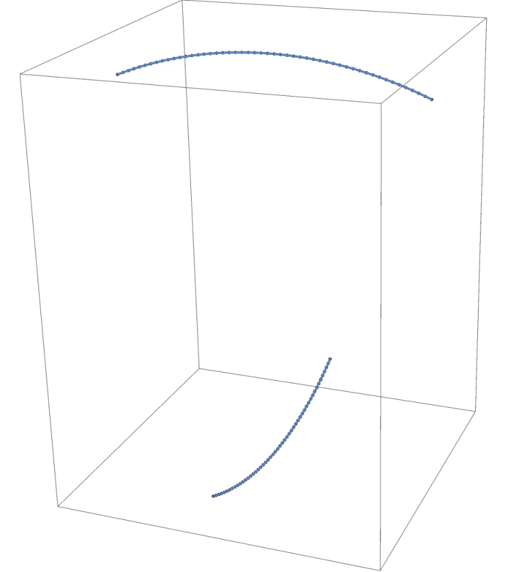
Refer to caption
Figure 3. The set X:X: two opposing arcs from unit circles.

We present an example of a subset of ℝ3\mathbb{R}^{3} with subsets of size nn that appear to have ≈n1.5\approx n^{1.5} 𝑃𝐻\mathit{PH} intervals. This example was suggested by Herbert Edelsbrunner.

Let C1C_{1} and C2C_{2} be the following arcs from unit circles in ℝ3:\mathbb{R}^{3}:

C1={(cos(θ),sin(θ),0):θ∈[−π/8,π/8]}C_{1}=\left\{\left(\cos\left(\theta\right),\sin\left(\theta\right),0\right):\theta\in\left[-\pi/8,\pi/8\right]\right\}
C2={(1−cos(θ),0,sin(θ)):θ∈[−π/8,π/8]}C_{2}=\left\{\left(1-\cos\left(\theta\right),0,\sin\left(\theta\right)\right):\theta\in\left[-\pi/8,\pi/8\right]\right\}

and let X=C1∪C2.X=C_{1}\cup C_{2}. XX is shown in Figure 3. Let xn⊂X\textbf{x}_{n}\subset X be a point set obtained by placing ⌊n/2⌋\lfloor n/2\rfloor uniformly spaced points on each of the two circular arcs. Computations indicate that |𝑃𝐻i​(xn)|≈|xn|1.5\left|\mathit{PH}_{i}\left(\textbf{x}_{n}\right)\right|\approx\left|\textbf{x}_{n}\right|^{1.5} for i=1,2i=1,2 (Figure 4), but that E11​(xn)E_{1}^{1}\left(\textbf{x}_{n}\right) and E12​(xn)E_{1}^{2}\left(\textbf{x}_{n}\right) are bounded as functions of nn (Figure 4). As such, the question remains of whether the 𝑃𝐻i\mathit{PH}_{i} dimension is bounded above by the upper box dimension for any subset of Euclidean space. This example suggests that it may be necessary to bound the number of “long” intervals of a “well-spaced” point set rather than the total number of intervals to achieve a sharp result.

Refer to caption
Refer to caption
Figure 4. (a) The number of 𝑃𝐻1\mathit{PH}_{1} intervals of xn,\textbf{x}_{n}, which appears to grow approximately as n1.5.n^{1.5}. The data for 𝑃𝐻2\mathit{PH}_{2} is similar. (b) The quantities E11​(xn)E_{1}^{1}\left(\textbf{x}_{n}\right) and E12​(Xn),E_{1}^{2}\left(X_{n}\right), which appear to be bounded as a function of n.n. Persistent homology was computed by calculating the alpha complex with CGAL [29] and passing the resulting filtration to JPLEX [26].

4. A Lower Bound

In this section, we prove the lower bounds in Theorems 8 and 9. However, we first consider the case of a bounded subset of Euclidean space with non-empty interior. Our later arguments will be more complicated, but have the same general outline.

Proposition 21.

If XX is a bounded subset of ℝm\mathbb{R}^{m} with non-empty interior then

dim𝑃𝐻i​(X)=m\begin{split}\text{dim}_{\mathit{PH}}^{i}\left(X\right)=m\end{split}

for i=0,…,m−1.i=0,\ldots,m-1.

Proof.

The upper bound was shown in Corollary 15.

Let 0≤i≤m−1.0\leq i\leq m-1. First, we compute the ii-dimensional persistent homology of the vertex set of the regular i+1i+1-simplex σ\sigma with edge length 2.\sqrt{2}. We may assume that the simplex is formed by the standard basis vectors e1,…,ei+1e_{1},\ldots,e_{i+1} in ℝi+1.\mathbb{R}^{i+1}. The circumcenter of σ\sigma is c≔(1i+1,…,1i+1),c\coloneqq\left(\frac{1}{i+1},\ldots,\frac{1}{i+1}\right), and the circumradius is

d⁡(ej,c)=(1−1/i)2+i(i+1)2=ii+1,d\left(e_{j},c\right)=\sqrt{\left(1-1/i\right)^{2}+\frac{i}{\left(i+1\right)^{2}}}=\sqrt{\frac{i}{i+1}}\,,

so σ\sigma enters the alpha complex Aϵ​(σ)A_{\epsilon}\left(\sigma\right) when ϵ=ii+1.\epsilon=\sqrt{\frac{i}{i+1}}. The same computation shows that the ii-dimensional faces of σ\sigma enter Aϵ​(σ)A_{\epsilon}\left(\sigma\right) when ϵ=i−1i=1−1i.\epsilon=\sqrt{\frac{i-1}{i}}=\sqrt{1-\frac{1}{i}}. Therefore, 𝑃𝐻i​(σ)\mathit{PH}_{i}\left(\sigma\right) consists of the single interval (1−1i,ii+1).\left(\sqrt{1-\frac{1}{i}},\sqrt{\frac{i}{i+1}}\right).

For convenience, let τ\tau be the length of the single 𝑃𝐻1\mathit{PH}_{1} interval of the regular i+1i+1-simplex with edge length 1,1,

τ=12​(ii+1−1−1i)\tau=\frac{1}{\sqrt{2}}\left(\sqrt{\frac{i}{i+1}}-\sqrt{1-\frac{1}{i}}\right)

and d^\hat{d} be the death-time of that interval,

d^=i2​i+2.\hat{d}=\sqrt{\frac{i}{2i+2}}\,.

XX has non-empty interior so we can find an mm-dimensional cube C⊂X.C\subset X. Rescale XX if necessary so that CC is a unit cube. Fix n∈ℕn\in\mathbb{N} and sub-divide CC into nmn^{m} cubes of width 1/n.1/n. Let C1,…,CtC_{1},\ldots,C_{t} be a maximal sub-collection of these cubes so that

(8) d⁡(Ck,Cl)>2​d^nd\left(C_{k},C_{l}\right)>2\frac{\hat{d}}{n}

for all k,l∈{1,…,t}k,l\in\left\{1,\ldots,t\right\} so that k≠lk\neq l (where d⁡(Ck,Cl)d\left(C_{k},C_{l}\right) is the minimum distance between any pair of points in the two cubes). There is a constant FF depending only on ii and mm so that t>F​nmt>Fn^{m} for all sufficiently large n.n.

For j=1,…,tj=1,\ldots,t find a regular i+1i+1-simplex of edge length 1n\frac{1}{n} inside each cube Cj.C_{j}. Let xj\textbf{x}_{j} be the vertices of this simplex, and let zn=∪j=1txj.\textbf{z}_{n}=\cup_{j=1}^{t}\textbf{x}_{j}. By Equation 8, the Čech complex on zn\textbf{z}_{n} equals the disjoint union of the Čech complexes on x1,…,xt\textbf{x}_{1},\ldots,\textbf{x}_{t} for any filtration value less than d^n\frac{\hat{d}}{n} (the first time an edge between a point in xj\textbf{x}_{j} and one in xk\textbf{x}_{k} can enter the complex for OPENj≠k).j\neq k). 𝑃𝐻i​(xj)\mathit{PH}_{i}\left(\textbf{x}_{j}\right) consist of a single interval of length 1n​τ\frac{1}{n}\tau that dies at time d^n.\frac{\hat{d}}{n}. It follows that 𝑃𝐻i​(zn)\mathit{PH}_{i}\left(\textbf{z}_{n}\right) contains at least F​nmFn^{m} intervals of length 1n​τ.\frac{1}{n}\tau.

Let α<m,\alpha<m, and compute

Eαi​(zn)≥F​nm​(τn)α=F​τα​nm−αE_{\alpha}^{i}\left(\textbf{z}_{n}\right)\geq Fn^{m}\left(\frac{\tau}{n}\right)^{\alpha}=F\tau^{\alpha}n^{m-\alpha}\,

which limits to ∞\infty as n→∞,n\rightarrow\infty, because α<m.\alpha<m. Therefore, dim𝑃𝐻i​(X)≥α\text{dim}_{\mathit{PH}}^{i}\left(X\right)\geq\alpha for any α<m\alpha<m and dim𝑃𝐻i​(X)=m,\text{dim}_{\mathit{PH}}^{i}\left(X\right)=m, as desired. ∎

In the preceding proof, we could find a cube in Euclidean space for which each sub-cube was occupied, and found point sets with non-trivial homology inside those cubes. If XX is a bounded subset of ℝm,\mathbb{R}^{m}, and dimbox​X<m,\text{dim}_{\text{box}}{X}<m, most cubes will not be occupied. As such, we need to proceed with care.

Let [N]\left[N\right] denote the integers 1,…,n1,\ldots,n and let [N]m⊂ℤm\left[N\right]^{m}\subset\mathbb{Z}^{m} be [N]×[N]×…×[N].\left[N\right]\times\left[N\right]\times\ldots\times\left[N\right]. For each x∈δ​ℤm,x\in\delta\mathbb{Z}^{m}, let the cube corresponding to xx be the cube of width δ\delta centered at x.x. The grid of mesh δ\delta is the set of all cubes in this tessellation. If XX is a bounded subset of ℝm,\mathbb{R}^{m}, the upper box dimension of XX controls the number of cubes in the grid of mesh δ\delta that intersect X.X. Our strategy to prove a lower bound for the 𝑃𝐻\mathit{PH} dimension of XX in terms of the upper box dimension is to show that a sufficiently large collection of points, each in a distinct cube of [N]m,\left[N\right]^{m}, must contain a subset with non-trivial persistent homology.

Figure 5. The 𝑃𝐻1\mathit{PH}_{1} class of the lattice points corresponding to the gray cubes in (a) and (b) is stable — any choice of one point in each cube will give the vertices of an acute triangle, and therefore a set with non-trivial 𝑃𝐻1.\mathit{PH}_{1}. The one in (c) and (d) is not, because the points in (d) form an obtuse triangle so the persistent homology of that set is trivial.
Definition 22.

x⊂ℤm\textbf{x}\subset\mathbb{Z}^{m} has a stable 𝑃𝐻i\mathit{PH}_{i}-class if any point collection y consisting of exactly one point in each cube corresponding to a point of x has a 𝑃𝐻i\mathit{PH}_{i} interval II so that |I|≥c\left|I\right|\geq c for some constant c>0c>0 (see Figure 5). The supremal such cc is called the size of the stable persistence class.

The stability of the bottleneck distance immediately implies the following.

Proposition 23.

If x⊂ℤm\textbf{x}\subset\mathbb{Z}^{m} and there is an interval I∈𝑃𝐻i​(x)I\in\mathit{PH}_{i}\left(\textbf{x}\right) with

|I|>m+ϵ,\begin{split}\left|I\right|>\sqrt{m}+\epsilon\,,\end{split}

then x has a stable 𝑃𝐻i\mathit{PH}_{i}-class of size at least ϵ.\epsilon.

Proof.

If x and y are in Definition 22, then dH​(x,y)<m/2,d_{H}\left(\textbf{x},\textbf{y}\right)<\sqrt{m}/2, the maximal distance between a point in a unit cube and the center of that cube. By bottleneck stability, 𝑃𝐻i​(y)\mathit{PH}_{i}\left(\textbf{y}\right) has an interval of length at least ϵ.\epsilon. ∎

Definition 24.

Let ξim​(N)\xi_{i}^{m}\left(N\right) be the size of the largest subset x of [N]m\left[N\right]^{m} so that no subset y of x has a stable 𝑃𝐻i\mathit{PH}_{i}-class of size greater than 1. That is, ξim​(N)\xi_{i}^{m}\left(N\right) is the smallest integer so that if |x|>ξim​(N),\left|\textbf{x}\right|>\xi_{i}^{m}\left(N\right), then there exist a y⊂x\textbf{y}\subset\textbf{x} with a stable 𝑃𝐻i\mathit{PH}_{i} class. Define

γim=lim infN→∞log⁡(ξim​(N))log⁡(N).\gamma_{i}^{m}=\liminf_{N\rightarrow\infty}\frac{\log\left(\xi_{i}^{m}\left(N\right)\right)}{\log\left(N\right)}\,.

The following proposition is stated for the Čech complex and γim\gamma_{i}^{m} is defined for that filtration, but an analogous result holds for the Rips complex (though the corresponding constant γ^im\hat{\gamma}_{i}^{m} may be different).

Proposition 25.

If XX is a bounded subset of ℝm\mathbb{R}^{m} and dimbox​(X)>γim\text{dim}_{\text{box}}\left(X\right)>\gamma_{i}^{m} then

dim𝑃𝐻1​(X)≥dimbox​(X).\begin{split}\text{dim}_{\mathit{PH}}^{1}\left(X\right)\geq\text{dim}_{\text{box}}\left(X\right)\,.\end{split}

Before proving this proposition, we introduce notation and state a technical lemma related to box-counting. The notation is illustrated in Figure 6. For δ∈ℝ,\delta\in\mathbb{R}, let ℬδ\mathcal{B}_{\delta} be the collection of cubes in the grid of mesh δ\delta in ℝm\mathbb{R}^{m} that intersect X.X. Also, if k∈ℕ,k\in\mathbb{N}, consider the larger cubes ℬk​δ.\mathcal{B}_{k\delta}. Note that each cube of ℬδ\mathcal{B}_{\delta} is contained in a unique cube of ℬk​δ,\mathcal{B}_{k\delta}, and each cube of ℬk​δ\mathcal{B}_{k\delta} contains at least one cube of ℬδ.\mathcal{B}_{\delta}. If C∈ℬk​δ,C\in\mathcal{B}_{k\delta}, let

𝒞k​(C)={B∈ℬδ:B⊂C}.\mathcal{C}_{k}\left(C\right)=\left\{B\in\mathcal{B}_{\delta}:B\subset C\right\}\,.
Refer to caption
Figure 6. The box notation used in the proofs of Proposition 25 and Lemma 26.

Furthermore, for λ>0\lambda>0 define

𝒟δ,kλ={C∈ℬk​δ:|𝒞k​(C)|>kλ}.\mathcal{D}^{\lambda}_{\delta,k}=\left\{C\in\mathcal{B}_{k\delta}:\left|\mathcal{C}_{k}\left(C\right)\right|>k^{\lambda}\right\}\,.

The idea of the proof of Proposition 25 is to choose kk and λ\lambda so that we can find a set of points in every cube 𝒟δ,kλ\mathcal{D}^{\lambda}_{\delta,k} that has a stable 𝑃𝐻i\mathit{PH}_{i} class, and show that δα​|𝒟δ,kλ|→∞\delta^{\alpha}\left|\mathcal{D}^{\lambda}_{\delta,k}\right|\rightarrow\infty for α<dimbox​(X).\alpha<\text{dim}_{\text{box}}\left(X\right). This is a little tricky as, the definition of the upper box dimension only gives us weak control over the asymptotics of |ℬδ|.\left|\mathcal{B}_{\delta}\right|. As such, we cannot choose a fixed value of kk and must instead let kk increase slowly as δ→0.\delta\rightarrow 0.

Lemma 26.

If XX is a bounded subset of ℝm\mathbb{R}^{m} and α<λ<dimbox​(X),\alpha<\lambda<\text{dim}_{\text{box}}\left(X\right), there exist a sequence of real numbers δj→0\delta_{j}\rightarrow 0 and a sequence of natural numbers kj→∞k_{j}\rightarrow\infty so that

δjα​|ℬδj,kjλ|→∞.\delta_{j}^{\alpha}\left|\mathcal{B}^{\lambda}_{\delta_{j},k_{j}}\right|\rightarrow\infty\,.

We prove Proposition 25 first, then return to the proof of Lemma 26.

Proof of Propostion 25.

Let d=dimbox​(X)d=\text{dim}_{\text{box}}\left(X\right) and α<d.\alpha<d. We will find finite point collections zj⊂X\textbf{z}_{j}\subset X so that Eαi​(zj)→∞E^{i}_{\alpha}\left(\textbf{z}_{j}\right)\rightarrow\infty as j→∞.j\rightarrow\infty. Choose λ\lambda so that

max​(γim,α)<λ<d.\text{max}\left(\gamma_{i}^{m},\alpha\right)<\lambda<d\,.

By the previous lemma, there are sequences of real numbers δj→0\delta_{j}\rightarrow 0 and kj→∞k_{j}\rightarrow\infty so that

δjα​|𝒟δj,kjλ|→∞\delta_{j}^{\alpha}\left|\mathcal{D}^{\lambda}_{\delta_{j},k_{j}}\right|\rightarrow\infty

Each cube C∈𝒟δj,kjλC\in\mathcal{D}^{\lambda}_{\delta_{j},k_{j}} contains at least kjλk_{j}^{\lambda} sub-cubes of width δj\delta_{j} that intersect X.X. λ>γim,\lambda>\gamma_{i}^{m}, so for sufficiently large kjk_{j} we can find a finite point set x​(C)∈X∩C\textbf{x}\left(C\right)\in X\cap C so that 𝑃𝐻i​(x​(C))\mathit{PH}_{i}\left(\textbf{x}\left(C\right)\right) has an interval of length at least δj.\delta_{j}. To combine the contributions of multiple points sets x​(C)\textbf{x}\left(C\right), we must thin the collection 𝒟δj,kjλ.\mathcal{D}^{\lambda}_{\delta_{j},k_{j}}.

Let {C1,…,Ct}\left\{C_{1},\ldots,C_{t}\right\} be a maximal collection of cubes in 𝒟δj,kjλ\mathcal{D}^{\lambda}_{\delta_{j},k_{j}} so that d⁡(Ck,Cl)>2​kj​δj​md\left(C_{k},C_{l}\right)>2k_{j}\delta_{j}\sqrt{m} for all k,l∈{1,…,t}k,l\in\left\{1,\ldots,t\right\} so that k≠lk\neq l (where d⁡(Ck,Cl)d\left(C_{k},C_{l}\right) is the minimum distance between any pair of points in the two cubes). There is a constant FF depending only on the ambient dimension mm so that t≥F​|𝒟δj,kjλ|t\geq F\left|\mathcal{D}^{\lambda}_{\delta_{j},k_{j}}\right| for sufficiently large j.j.

Let zj=∪k=1tx(Ck).\textbf{z}_{j}=\cup_{k=1}^{t}\textbf{x}\left(C_{k}\right). By construction, the Čech complex on zj\textbf{z}_{j} equals the disjoint union of the Čech complexes on x​(C1),…,x​(Ct)\textbf{x}\left(C_{1}\right),\ldots,\textbf{x}\left(C_{t}\right) for any filtration value less than kj​δj​m.k_{j}\delta_{j}\sqrt{m}. Furthermore, the diameter of each set x​(Ck)\textbf{x}\left(C_{k}\right) is less than kj​δj​mk_{j}\delta_{j}\sqrt{m} so any interval (b0,d0)∈𝑃𝐻i​(x​(Ck))(b_{0},d_{0})\in\mathit{PH}_{i}\left(\textbf{x}\left(C_{k}\right)\right) satisfies d0<kj​δj​m.d_{0}<k_{j}\delta_{j}\sqrt{m}. Therefore, as sets of intervals, we have that ∪kPHi(x(Ck))⊆𝑃𝐻i(zj).\cup_{k}PH_{i}\left(\textbf{x}\left(C_{k}\right)\right)\subseteq\mathit{PH}_{i}\left(\textbf{z}_{j}\right). It follows that 𝑃𝐻i​(zj)\mathit{PH}_{i}\left(\textbf{z}_{j}\right) contains at tt intervals of length greater than δj.\delta_{j}.

Therefore,

Eαi​(zj)≥t​δjα≥F​|𝒟δj,kjλ|​δjα,E_{\alpha}^{i}\left(\textbf{z}_{j}\right)\geq t\delta_{j}^{\alpha}\geq F\left|\mathcal{D}^{\lambda}_{\delta_{j},k_{j}}\right|\delta_{j}^{\alpha}\,,

which goes to ∞\infty as j→∞j\rightarrow\infty by the previous lemma. Thus dim𝑃𝐻i​(X)≥α\text{dim}_{\mathit{PH}}^{i}\left(X\right)\geq\alpha for all α<d,\alpha<d, and dim𝑃𝐻i​(X)≥d\text{dim}_{\mathit{PH}}^{i}\left(X\right)\geq d as desired. ∎

Proof of Lemma 26.

Let d=dimbox​(X),d=\text{dim}_{\text{box}}\left(X\right), and choose 0<p<10<p<1 so that d−p​m>α.d-pm>\alpha. Also, choose

ϵ<min​(2​(d−p​m−α),p​d−p​λ).\epsilon<\text{min}\left(2\left(d-pm-\alpha\right),pd-p\lambda\right)\,.

Let β=d+ϵ/2,\beta=d+\epsilon/2, and note for future reference that

(9) α+p​m−β+ϵ=α+p​m−d+ϵ/2<0\alpha+pm-\beta+\epsilon=\alpha+pm-d+\epsilon/2<0

and

(10) p​β−p​λ−ϵ=p​d−p​λ−(1−p/2)​ϵ>p​d−p​λ−ϵ>0.p\beta-p\lambda-\epsilon=pd-p\lambda-\left(1-p/2\right)\epsilon>pd-p\lambda-\epsilon>0\,.

β>d\beta>d so there exists a δ0>0\delta_{0}>0 so that |Bδ|<δ−β\left|B_{\delta}\right|<\delta^{-\beta} for all δ<δ0.\delta<\delta_{0}. Also, β−ϵ<d\beta-\epsilon<d so there exists a sequence δj→0\delta_{j}\rightarrow 0 so that |Bδj|>δj−β+ϵ\left|B_{\delta_{j}}\right|>\delta_{j}^{-\beta+\epsilon} for all j∈ℕ.j\in\mathbb{N}. We may assume that δj<δ0\delta_{j}<\delta_{0} for all j.j. Let

(11) kj=⌊δj−p⌋.k_{j}=\lfloor\delta_{j}^{-p}\rfloor\,.

A cube in ℬkj​δj\mathcal{B}_{k_{j}\delta_{j}} can contain at most kjmk_{j}^{m} cubes in ℬδj,\mathcal{B}_{\delta_{j}}, and every cube in ℬδj\mathcal{B}_{\delta_{j}} is contained in exactly one cube ℬkj​δj.\mathcal{B}_{k_{j}\delta_{j}}. It follows that 𝒟δj,kjλ\mathcal{D}^{\lambda}_{\delta_{j},k_{j}} is greater than or equal to the smallest integer aa so that

a​kjm+(|ℬkj​δj|−a)​kjλ≥|Bδj|.ak_{j}^{m}+\left(\left|\mathcal{B}_{k_{j}\delta_{j}}\right|-a\right)k_{j}^{\lambda}\geq\left|B_{\delta_{j}}\right|\,.

Rearranging terms, we have that

a≥\displaystyle a\geq |Bδj|−|Bkj​δj|​kjλkjm−kjλ\displaystyle\;\;\frac{\left|B_{\delta_{j}}\right|-\left|B_{k_{j}\delta_{j}}\right|k_{j}^{\lambda}}{k_{j}^{m}-k_{j}^{\lambda}}
=\displaystyle= |Bδj|​kj−λ−|Bkj​δj|kjm−λ−1\displaystyle\;\;\frac{\left|B_{\delta_{j}}\right|k_{j}^{-\lambda}-\left|B_{k_{j}\delta_{j}}\right|}{k_{j}^{m-\lambda}-1}
≥\displaystyle\geq δj−β+ϵ​kj−λ−kj−β​δj−βkjm−λ−1\displaystyle\;\;\frac{\delta_{j}^{-\beta+\epsilon}k_{j}^{-\lambda}-k_{j}^{-\beta}\delta_{j}^{-\beta}}{k_{j}^{m-\lambda}-1}
=\displaystyle= δj−β+ϵ​⌊δj−p⌋−λ−⌊δj−p⌋−β​δj−β⌊δj−p⌋m−λ−1\displaystyle\;\;\frac{\delta_{j}^{-\beta+\epsilon}\lfloor\delta_{j}^{-p}\rfloor^{-\lambda}-\lfloor\delta_{j}^{-p}\rfloor^{-\beta}\delta_{j}^{-\beta}}{\lfloor\delta_{j}^{-p}\rfloor^{m-\lambda}-1} by Eqn. 11
≈\displaystyle\approx δjp​λ−β+ϵ−δjp​β−βδp​λ−p​m−1\displaystyle\;\;\frac{\delta_{j}^{p\lambda-\beta+\epsilon}-\delta_{j}^{p\beta-\beta}}{\delta^{p\lambda-pm}-1} as δj→0\delta_{j}\rightarrow 0
≈\displaystyle\approx δjp​m−β+ϵ,\displaystyle\;\;\delta_{j}^{pm-\beta+\epsilon}\,,\

where we used that p​λ−β+ϵ>p​β−βp\lambda-\beta+\epsilon>p\beta-\beta by Equation 10.

Choose a JJ so that if j>J,j>J,

|𝒟δj,kjλ|≥12​δjp​m−β+ϵ.\left|\mathcal{D}^{\lambda}_{\delta_{j},k_{j}}\right|\geq\frac{1}{2}\delta_{j}^{pm-\beta+\epsilon}\,.

Then, if j>J,j>J,

δjα​|𝒟δj,kjλ|≥12​δjα​δjp​m−β+ϵ=12​δjα+p​m−β+ϵ,\delta_{j}^{\alpha}\left|\mathcal{D}^{\lambda}_{\delta_{j},k_{j}}\right|\geq\frac{1}{2}\delta_{j}^{\alpha}\delta_{j}^{pm-\beta+\epsilon}=\frac{1}{2}\delta_{j}^{\alpha+pm-\beta+\epsilon}\,,

which by equation Equation 9, limits to ∞\infty as j→∞.j\rightarrow\infty. ∎

4.1. A Bound for γ1m\gamma_{1}^{m}

We prove an upper bound for γ1m\gamma_{1}^{m} by considering the contribution of small triangles to the persistent homology of a subset of ℤm.\mathbb{Z}^{m}. Three points in Euclidean space give rise to a 𝑃𝐻1\mathit{PH}_{1}-class if and only if they are the vertices of an acute triangle, in which case the total persistence (death minus birth) equals the circumradius minus half the length of its longest edge.

Proposition 27.
γ1m≥m−1/2.\gamma_{1}^{m}\geq m-1/2\,.
Proof.

We will prove that ξ1m​(N)∈O⁡(Nm−1/2)\xi_{1}^{m}\left(N\right)\in O\left(N^{m-1/2}\right) by showing that if X⊂[N]m,X\subset\left[N\right]^{m},

X⊂[N]m,c>4​m+4,|X|>8​c​Nm−1/2+4​Nm−1,X\subset\left[N\right]^{m},\qquad c>\sqrt{4\sqrt{m}+4},\qquad\left|X\right|>8cN^{m-1/2}+4N^{m-1},

and NN is sufficiently large then there exist three points p1,q2,p_{1},q_{2}, and q3q_{3} of XX so that 𝑃𝐻1​({p1,q2,q3})\mathit{PH}_{1}\left(\left\{p_{1},q_{2},q_{3}\right\}\right) contains an interval of length at least 1+m.1+\sqrt{m}. The desired result will then follow from Proposition 23.

First, we reduce the problem to a two-dimensional one. If m>2,m>2, we may find a two-dimensional slice SS of [N]m\left[N\right]^{m} of the form [N]2×w,\left[N\right]^{2}\times w, so that the density of XX in SS is greater than or equal to the density of XX in [N]m.\left[N\right]^{m}. That is,

(12) |X∩S|≥N2​|X|Nm>8​c​N1.5+4​N.\left|X\cap S\right|\geq N^{2}\frac{\left|X\right|}{N^{m}}>8cN^{1.5}+4N\,.

We will treat SS as a two-dimensional grid of mm-dimensional cubes, with NN rows and NN columns, as in Figure 7.

Refer to caption
Figure 7. The setup in Proposition 27. The points of XX are shown in gray, and the triangle formed by the points p1,p_{1}, q2,q_{2}, and q3q_{3} is shown by the red dashed lines. It is an acute triangle, and the triangle q1,q2,q_{1},q_{2}, and q3q_{3} is either acute or right.

Let R1,…,RNR_{1},\ldots,R_{N} be the rows of [N]2\left[N\right]^{2} and C1​…​CNC_{1}\ldots C_{N} the the columns. Let 1≤j≤N.1\leq j\leq N. If |X∩Rj|>4​c​N+2,\left|X\cap R_{j}\right|>4c\sqrt{N}+2, let AjA_{j} be the set of 4​c​N+24c\sqrt{N}+2 elements of X∩RjX\cap R_{j} that contains the leftmost 2​c​N+12c\sqrt{N}+1 elements of X∩RjX\cap R_{j} and the rightmost 2​c​N+12c\sqrt{N}+1 elements of X∩Rj.X\cap R_{j}. Otherwise, let Aj=X∩Rj.A_{j}=X\cap R_{j}. Similarly, if |X∩Cj|>4​c​N+2,\left|X\cap C_{j}\right|>4c\sqrt{N}+2, let BjB_{j} be the set of 4​c​N+24c\sqrt{N}+2 elements of X∩CjX\cap C_{j} that contains the uppermost 2​c​N+12c\sqrt{N}+1 elements of X∩CjX\cap C_{j} and the lowermost 2​c​N+12c\sqrt{N}+1 elements of X∩Cj.X\cap C_{j}. Otherwise, let Bj=X∩Cj.B_{j}=X\cap C_{j}. Then, if D=⋃j=1NAj∪Bj,D=\bigcup_{j=1}^{N}A_{j}\cup B_{j},

|D|≤2​N​(4​c​N+2)=8​c​N1.5+4​N<|X∩S|,\left|D\right|\leq 2N\left(4c\sqrt{N}+2\right)=8cN^{1.5}+4N<\left|X\cap S\right|\,,

by Equation 12. Therefore, X∩S∖D≠∅X\cap S\setminus D\neq\varnothing and there is a y∈X∩S∖D.y\in X\cap S\setminus D. The row of SS containing yy contains at least 2​c​N+12c\sqrt{N}+1 additional elements of X∩SX\cap S both to the left and to the right of y,y, and the column of SS containing yy has at least 2​c​N+12c\sqrt{N}+1 additional elements of X∩SX\cap S both above and below y.y. Let q1,q_{1}, q2,q_{2}, q3q_{3} and q4q_{4} be elements of XX to the right, above, below, and to the left of yy so that there c​Nc\sqrt{N} other elements of X∩SX\cap S between them and y,y, and at least c​Nc\sqrt{N} additional elements between them and the boundary of S.S. Translate SS so that yy is located at (0,0)\left(0,0\right) (ignoring the higher-dimensional coordinates). q1,q2,q3,q_{1},q_{2},q_{3}, and q4q_{4} form a quadrilateral, so there is a non-obtuse angle at at least one of the vertices. Without loss of generality, suppose the angle at q1q_{1} is non-obtuse. Let q1=(x^,0),q_{1}=\left(\hat{x},0\right), q2=(0,y1),q_{2}=\left(0,y_{1}\right), and q3=(0,y2).q_{3}=\left(0,y_{2}\right). By construction, x^\hat{x} and y1y_{1} are positive, and y2y_{2} is negative. Additionally, let p1=(x,0)p_{1}=\left(x,0\right) be an element of X∩SX\cap S in the same row as yy and q1q_{1} that is at least c​Nc\sqrt{N} cubes further to the right of q1.q_{1}. Then p1,q2,p_{1},q_{2}, and q3q_{3} form an acute triangle. See Figure 7.

p1,q2,p_{1},q_{2}, and q3q_{3} form an acute triangle, so 𝑃𝐻1​({p1,q2,q3})\mathit{PH}_{1}(\left\{p_{1},q_{2},q_{3}\right\}) consists of a single interval. We will show that the length of this interval is greater than 1+m1+\sqrt{m} for sufficiently large N,N, which will imply that the 𝑃𝐻1\mathit{PH}_{1} class is a stable class of size greater than one. The length of this interval is equal to the circumradius of the triangle minus half the length of its maximum edge. The circumradius of a triangle with edge lengths a,b,ca,b,c and area AA is a​b​c/4​Aabc/4A so the circumradius of p1,q2,q3p_{1},q_{2},q_{3} is

(x2+y12)​(x2+y22)​(y1−y2)4⁤12​(y1−y2)​x=(x2+y12)​(x2+y22)2​x.\frac{\sqrt{\left(x^{2}+y_{1}^{2}\right)\left(x^{2}+y_{2}^{2}\right)}\left(y_{1}-y_{2}\right)}{4\frac{1}{2}\left(y_{1}-y_{2}\right)x}=\frac{\sqrt{\left(x^{2}+y_{1}^{2}\right)\left(x^{2}+y_{2}^{2}\right)}}{2x}\,.

We consider three cases. In the first case, the edge from q2q_{2} to q3q_{3} is longest. In this case, the total persistence equals

T​P1​(x,y1,y2)=(x2+y12)​(x2+y22)2​x−y1−y22.TP_{1}\left(x,y_{1},y_{2}\right)=\frac{\sqrt{\left(x^{2}+y_{1}^{2}\right)\left(x^{2}+y_{2}^{2}\right)}}{2x}-\frac{y_{1}-y_{2}}{2}\,.

q1,q2,q3q_{1},q_{2},q_{3} is an acute triangle, so x^>−y1​y2\hat{x}>-y_{1}y_{2} and x>−y1​y2+c​N.x>\sqrt{-y_{1}y_{2}}+c\sqrt{N}. In Appendix B.1, we show that, subject to the constraints that c​N≤y1≤N,c\sqrt{N}\leq y_{1}\leq N, −N≤y2≤−c​N,-N\leq y_{2}\leq-c\sqrt{N}, and x>−y1​y2+c​Nx>\sqrt{-y_{1}y_{2}}+c\sqrt{N} (which all hold in this case),

T​P1​(x,y1,y2)≥T​P1​(c​N+N,N,−N)=c2​N2​(c​N+N)TP_{1}\left(x,y_{1},y_{2}\right)\geq TP_{1}\left(c\sqrt{N}+N,N,-N\right)=\frac{c^{2}N}{2\left(c\sqrt{N}+N\right)}

which is an increasing function of NN whose limit is 12​c2\frac{1}{2}c^{2} as NN goes to ∞.\infty. As c>4​m+4>2​m+2,c>\sqrt{4\sqrt{m}+4}>\sqrt{2\sqrt{m}+2}, the total persistence will exceed 1+m1+\sqrt{m} for sufficiently large N,N, as desired.

In the second case, the edge between pp and q1q_{1} is longest. In this case, the total persistence equals

T​P2​(x,y1,y2)=(x2+y12)​(x2+y22)2​x−x2+y122.TP_{2}\left(x,y_{1},y_{2}\right)=\frac{\sqrt{\left(x^{2}+y_{1}^{2}\right)\left(x^{2}+y_{2}^{2}\right)}}{2x}-\frac{\sqrt{x^{2}+y_{1}^{2}}}{2}\,.

As we show in Appendix B.2, for sufficiently large N,N, this is minimized when xx is as large as possible and the magnitudes of y1y_{1} and y2y_{2} are as small as possible. Thus, for sufficiently large N,N,

T​P2​(x,y1,y2)≥T​P2​(N,c​N,−c​N)=12​(c2+N−c2​N+N2)TP_{2}\left(x,y_{1},y_{2}\right)\geq TP_{2}\left(N,c\sqrt{N},-c\sqrt{N}\right)=\frac{1}{2}\left(c^{2}+N-\sqrt{c^{2}N+N^{2}}\right)

which is a decreasing function of NN with limiting value 14​c2.\frac{1}{4}c^{2}. Because c>4​m+4c>\sqrt{4\sqrt{m}+4}, the total persistence is always greater than 1+m,1+\sqrt{m}, as desired. The argument in the third case is identical to this one. ∎

The previous result, together with Proposition 25, completes the proofs of Theorems 8 and 9.

5. Results for the Rips Complex

In this section, we first construct an example where for which dim𝑃𝐻~1​(X)=2\text{dim}_{\widetilde{\mathit{PH}}_{1}}\left(X\right)=2 but dimbox​(X)=1,\text{dim}_{\text{box}}\left(X\right)=1, then we show that this cannot occur in Euclidean space by proving Theorems 10 and 11.

5.1. An Example

Here, we prove Proposition 6 by constructing an example of a metric space not embeddable in any Euclidean space whose 𝑃𝐻~1\widetilde{\mathit{PH}}_{1} dimension equals 2 but whose upper box dimension equals 1. This contrasts with the 𝑃𝐻~0\widetilde{\mathit{PH}}_{0} dimension, which was proven by Kozma, Lotker, and Stupp [20] to agree with the upper box dimension for all metric spaces. The rough idea of the construction is to build a space that includes a copies of the complete bipartite graph on 2n2^{n} vertices at different scales.

Proof of Proposition 6.

We will construct XX as the union of finite point sets Xn.X_{n}. For each n∈ℕn\in\mathbb{N} let XnX_{n} be the set consisting of 2n+12^{n+1} points x1n,x2n,…,x2nnx^{n}_{1},x^{n}_{2},\ldots,x^{n}_{2^{n}} and y1n,y2n,…,y2nn,y^{n}_{1},y^{n}_{2},\ldots,y^{n}_{2^{n}}, and let

d⁡(xin,yin)=12n+1d⁡(xin,xjn)=(1−δi,j)​12nd⁡(yin,yjn)=(1−δi,j)​12n.d\left(x^{n}_{i},y^{n}_{i}\right)=\frac{1}{2^{n+1}}\hskip 36.135ptd\left(x^{n}_{i},x^{n}_{j}\right)=\left(1-\delta_{i,j}\right)\frac{1}{2^{n}}\hskip 36.135ptd\left(y^{n}_{i},y^{n}_{j}\right)=\left(1-\delta_{i,j}\right)\frac{1}{2^{n}}\,.

Let X=∪i=0∞Xi.X=\cup_{i=0}^{\infty}X_{i}. if i≠j,i\neq j, z∈Xiz\in X_{i} and w∈Xj,w\in X_{j}, set

(13) d⁡(z,w)=12min​(i,j).d\left(z,w\right)=\frac{1}{2^{\text{min}\left(i,j\right)}}\,.

We will show the upper box dimension of XX equals one by computing Nδ​(X),N_{\delta}\left(X\right), the maximum number of disjoint closed balls of radius δ\delta centered at points of X.X.

Suppose 2−n−1<δ<2−n2^{-n-1}<\delta<2^{-n} and that the balls centered at x are a maximal collection of disjoint balls of radius δ\delta centered at points of X.X. Let Yn=∪j<nXjY_{n}=\cup_{j<n}X_{j} and Zn=∪j>nXj.Z_{n}=\cup_{j>n}X_{j}. If y∈Yn,y\in Y_{n}, Bδ​(y)B_{\delta}\left(y\right) contains every point of Yn,Y_{n}, but no point of X∖Yn.X\setminus Y_{n}. Therefore, x contains one point of Yn.Y_{n}. Also, for 1≤i≤2n,1\leq i\leq 2^{n}, Bδ​(yin)B_{\delta}\left(y^{n}_{i}\right) contains yiny^{n}_{i} and the 2n2^{n} points x1n,…,x2nn.x^{n}_{1},\ldots,x^{n}_{2^{n}}. By symmetry, Bδ​(xin)B_{\delta}\left(x^{n}_{i}\right) contains xinx^{n}_{i} and the 2n2^{n} points y1n,…,y2nn.y^{n}_{1},\ldots,y^{n}_{2^{n}}. Therefore, any two δ\delta-balls centered at points of XnX_{n} intersect and x contains either one point yiny^{n}_{i} or one point xin.x^{n}_{i}. Finally, if z∈Zn,z\in Z_{n}, Bδ​(z)∩X=z.B_{\delta}\left(z\right)\cap X=z. Therefore, x must contain all of the points of Zn.Z_{n}. It follows that

Nδ​(X)=\displaystyle N_{\delta}\left(X\right)= |x|\displaystyle\;\;\left|\textbf{x}\right|
=\displaystyle=   1+2n+|Zn|\displaystyle\;\;1+2^{n}+\left|Z_{n}\right|
=\displaystyle=   1+∑j=0n−1|Xn|\displaystyle\;\;1+\sum_{j=0}^{n-1}\left|X_{n}\right|
=\displaystyle=   1+∑j=0n−12n+1\displaystyle\;\;1+\sum_{j=0}^{n-1}2^{n+1}
=\displaystyle=    2n+1−1\displaystyle\;\;\ 2^{n+1}-1
=\displaystyle=   2−⌈log⁡(δ)+1log⁡(2)⌉−1.\displaystyle\;\;2^{-\lceil\frac{\log\left(\delta\right)+1}{\log\left(2\right)}\rceil}-1\,.

Therefore

dimbox​(X)=\displaystyle\text{dim}_{\text{box}}\left(X\right)= lim supδ→0log⁡(Nδ​(X))−log⁡(δ)\displaystyle\;\;\limsup_{\delta\rightarrow 0}{\frac{\log\left(N_{\delta}\left(X\right)\right)}{-\log\left(\delta\right)}}
=\displaystyle= limδ→0log⁡(2−⌈log⁡(δ)log⁡(2)⌉+1−1)−log⁡(δ)\displaystyle\;\;\lim_{\delta\rightarrow 0}\frac{\log\left(2^{-\lceil\frac{\log\left(\delta\right)}{\log\left(2\right)}\rceil+1}-1\right)}{-\log\left(\delta\right)}
=\displaystyle= limδ→0−⌈log⁡(δ)log⁡(2)⌉​log⁡(2)−log⁡(δ)\displaystyle\;\;\lim_{\delta\rightarrow 0}\frac{-\lceil\frac{\log\left(\delta\right)}{\log\left(2\right)}\rceil\log\left(2\right)}{-\log\left(\delta\right)}
=\displaystyle=   1.\displaystyle\;\;1\,.

On the other hand, consider the Rips complex ℛϵ​(Xn)\mathcal{R}_{\epsilon}\left(X_{n}\right) on Xn.X_{n}. There are three regimes. If ϵ<12n+1,\epsilon<\frac{1}{2^{n+1}}, then ℛϵ​(Xn)\mathcal{R}_{\epsilon}\left(X_{n}\right) consists of 2n+12^{n+1} 00-cells. When ϵ=12n+1,\epsilon=\frac{1}{2^{n+1}}, the 22​n2^{2n} edges between the points {xin}i=12n\left\{x_{i}^{n}\right\}_{i=1^{2^{n}}} and {yin}i=12n\left\{y_{i}^{n}\right\}_{i=1^{2^{n}}} enter the complex. The complex remains unchanged until ϵ=12n,\epsilon=\frac{1}{2^{n}}, when all possible simplices enter the complex and it becomes contractible. As such, all intervals of P​H~1​(Xn)\widetilde{PH}_{1}\left(X_{n}\right) are born at ϵ=12n+1\epsilon=\frac{1}{2^{n+1}} and die at ϵ=12n.\epsilon=\frac{1}{2^{n}}. By an Euler characteristic argument, there are 22​n−2n+1+12^{2n}-2^{n+1}+1 such intervals. Therefore, for α>0\alpha>0

E~α1​(Xn)=\displaystyle\widetilde{E}^{1}_{\alpha}\left(X_{n}\right)= (22​n−2n+1+1)​(12n−12n+1)α\displaystyle\;\;\left(2^{2n}-2^{n+1}+1\right)\left(\frac{1}{2^{n}}-\frac{1}{2^{n+1}}\right)^{\alpha}
=\displaystyle= (22​n−2n+1+1)​12α​n+α\displaystyle\;\;\left(2^{2n}-2^{n+1}+1\right)\frac{1}{2^{\alpha n+\alpha}}
=\displaystyle=   2−α​(2(2−α)​n−2(1−α)​n+1+2−α​n)\displaystyle\;\;2^{-\alpha}\left(2^{\left(2-\alpha\right)n}-2^{\left(1-\alpha\right)n+1}+2^{-\alpha n}\right)
≈\displaystyle\approx   2−α​2(2−α)​n,\displaystyle\;\;2^{-\alpha}2^{\left(2-\alpha\right)n}\,,

which is which is unbounded as n→∞n\rightarrow\infty if α<2.\alpha<2. Thus dim𝑃𝐻~1​(X)≥2.\text{dim}_{\widetilde{\mathit{PH}}_{1}}(X)\geq 2.

The argument that dim𝑃𝐻~1​(X)≤2\text{dim}_{\widetilde{\mathit{PH}}_{1}}(X)\leq 2 is similar but slightly trickier. Let α>2,\alpha>2, x⊆X,\textbf{x}\subseteq X, and xn=x∩Xn.\textbf{x}_{n}=\textbf{x}\cap X_{n}. An argument nearly identical to the previous one shows that P​H~1​(xn)\widetilde{PH}_{1}\left(\textbf{x}_{n}\right) consists of at most 22​n−2n+1+12^{2n}-2^{n+1}+1 intervals of the form (12n+1,12n),\left(\frac{1}{2^{n+1}},\frac{1}{2^{n}}\right), and

(14) E~α1​(xn)<2−α​(2(2−α)​n+2−α​n).\widetilde{E}^{1}_{\alpha}\left(\textbf{x}_{n}\right)<2^{-\alpha}\left(2^{\left(2-\alpha\right)n}+2^{-\alpha n}\right)\,.

We will show that we can write

E~α1​(x)=∑n=0∞E~α1​(xn).\widetilde{E}^{1}_{\alpha}\left(\textbf{x}\right)=\sum_{n=0}^{\infty}\widetilde{E}_{\alpha}^{1}\left(\textbf{x}_{n}\right)\,.

Let n∈ℕn\in\mathbb{N} and define

Ki,n​(Y)={(b,d)∈𝑃𝐻~i​(Y):12n+1≤b<12n}.K_{i,n}\left(Y\right)=\left\{\left(b,d\right)\in\widetilde{\mathit{PH}}_{i}\left(Y\right):\frac{1}{2^{n+1}}\leq b<\frac{1}{2^{n}}\right\}\,.

Also, let

12n+1≤ϵ<12n,yn=∪j<nxj, and zn=∪j>nxj.\frac{1}{2^{n+1}}\leq\epsilon<\frac{1}{2^{n}},\quad\textbf{y}_{n}=\cup_{j<n}\textbf{x}_{j},\text{ and }\textbf{z}_{n}=\cup_{j>n}\textbf{x}_{j}\,.

By equation 13, ℛϵ​(x)\mathcal{R}_{\epsilon}\left(\textbf{x}\right) contains no edges between points of yn\textbf{y}_{n} and points of xn.\textbf{x}_{n}. Furthermore, no point of zn\textbf{z}_{n} is contained in an edge. Therefore,

ℛϵ​(x)=ℛϵ​(xn)⊔ℛϵ​(yn)⊔ℛϵ​(zn),\mathcal{R}_{\epsilon}\left(\textbf{x}\right)=\mathcal{R}_{\epsilon}\left(\textbf{x}_{n}\right)\sqcup\mathcal{R}_{\epsilon}\left(\textbf{y}_{n}\right)\sqcup\mathcal{R}_{\epsilon}\left(\textbf{z}_{n}\right)\,,

where ⊔\sqcup denotes a disjoint union. ℛϵ​(yn)\mathcal{R}_{\epsilon}\left(\textbf{y}_{n}\right) is contractible because it contains all possible simplices, so H1​(ℛϵ​(yn))=0.H_{1}\left(\mathcal{R}_{\epsilon}\left(\textbf{y}_{n}\right)\right)=0. H1​(ℛϵ​(zn))H_{1}\left(\mathcal{R}_{\epsilon}\left(\textbf{z}_{n}\right)\right) is also trivial because ℛϵ​(zn)\mathcal{R}_{\epsilon}\left(\textbf{z}_{n}\right) contains only zero cells. Therefore, H1​(ℛϵ​(x))=H1​(ℛϵ​(xn)).H_{1}\left(\mathcal{R}_{\epsilon}\left(\textbf{x}\right)\right)=H_{1}\left(\mathcal{R}_{\epsilon}\left(\textbf{x}_{n}\right)\right). Also, if δ>12n\delta>\frac{1}{2^{n}} then ℛδ​(xn)\mathcal{R}_{\delta}\left(\textbf{x}_{n}\right) is contractible so the inclusion map H1​(ℛϵ​(x))→H1​(ℛδ​(x))H_{1}\left(\mathcal{R}_{\epsilon}\left(\textbf{x}\right)\right)\rightarrow H_{1}\left(\mathcal{R}_{\delta}\left(\textbf{x}\right)\right) is trivial. It follows that

(15) K1,n​(x)=K1,n​(xn)=𝑃𝐻^1​(xn).K_{1,n}\left(\textbf{x}\right)=K_{1,n}\left(\textbf{x}_{n}\right)=\widehat{\mathit{PH}}_{1}\left(\textbf{x}_{n}\right)\,.

Let α>2\alpha>2 and compute

E~α1​(x)=\displaystyle\widetilde{E}^{1}_{\alpha}\left(\textbf{x}\right)= ∑n∈ℕ∑I∈K1,n​(x)|I|α\displaystyle\;\;\sum_{n\in\mathbb{N}}\sum_{I\in K_{1,n}\left(\textbf{x}\right)}\left|I\right|^{\alpha}
=\displaystyle= ∑n∈ℕ∑I∈P​H^1​(xn)|I|α\displaystyle\;\;\sum_{n\in\mathbb{N}}\sum_{I\in\widehat{PH}_{1}\left(\textbf{x}_{n}\right)}\left|I\right|^{\alpha} by Eqn 15
=\displaystyle= ∑n∈ℕE~α1​(xn)\displaystyle\;\;\sum_{n\in\mathbb{N}}\widetilde{E}^{1}_{\alpha}\left(\textbf{x}_{n}\right)
≤\displaystyle\leq ∑n∈ℕ2−α​(2(2−α)​n+2−α​n)\displaystyle\;\;\sum_{n\in\mathbb{N}}2^{-\alpha}\left(2^{\left(2-\alpha\right)n}+2^{-\alpha n}\right) by Eqn 14
=\displaystyle=   2−α​(11−2(2−α)+11+2−α)\displaystyle\;\;2^{-\alpha}\left(\frac{1}{1-2^{\left(2-\alpha\right)}}+\frac{1}{1+2^{-\alpha}}\right) because α>2.\alpha>2\,.

Therefore E~α1​(x)\widetilde{E}^{1}_{\alpha}\left(\textbf{x}\right) is uniformly bounded for all x⊂X\textbf{x}\subset X when α>2,\alpha>2, and dim𝑃𝐻~1​(X)=2.\text{dim}_{\widetilde{\mathit{PH}}_{1}}\left(X\right)=2. ∎

5.2. A Bound for dim𝑃𝐻~1\text{dim}_{\widetilde{\mathit{PH}}_{1}}

We prove an upper bound for the 𝑃𝐻~1\widetilde{\mathit{PH}}_{1}-dimension of a subset of ℝm\mathbb{R}^{m} that does not depend on the ambient Euclidean dimension. Note that the proof of Proposition 18 (and the preceding lemmas) works for persistent homology defined in terms of either the Čech complex or the Rips complex.

The following argument is a modified version of the proof of Theorem 3.1 in Goff [16], which bounds the (non-persistent) first Betti number of a Rips complex of a finite point set in ℝm\mathbb{R}^{m} in terms of the kissing number KmK_{m} of ℝm.\mathbb{R}^{m}. Recall that KmK_{m} is the maximum number of disjoint unit spheres that can be tangent to a shared unit sphere. For example K1=2,K2=6,K_{1}=2,K_{2}=6, and K3=12.K_{3}=12. There is an expansive literature on upper and lower bounds for KmK_{m} [24], but here will we just need that KmK_{m} is finite.

Let ℛϵ​(X)\mathcal{R}_{\epsilon}\left(X\right) be the Rips complex of XX at parameter ϵ.\epsilon. For a 00-cell xx let Sϵ​(x)S_{\epsilon}\left(x\right) denote the star of xx

Sϵ​(x)={σ∈ℛϵ​(X):x∈σ},S_{\epsilon}\left(x\right)=\left\{\sigma\in\mathcal{R}_{\epsilon}\left(X\right):x\in\sigma\right\}\,,

and Lϵ⁡(x)L_{\epsilon\left(x\right)} denote the link of xx

Lϵ​(x)={(z1,…​zk)∈ℛϵ​(X):(x,z1,…​zk)∈ℛϵ​(X)}.L_{\epsilon}(x)=\left\{\left(z_{1},\ldots z_{k}\right)\in\mathcal{R}_{\epsilon}\left(X\right):\left(x,z_{1},\ldots z_{k}\right)\in\mathcal{R}_{\epsilon}\left(X\right)\right\}\,.

Sϵ⁡(x)S_{\epsilon\left(x\right)} is contractible.

Refer to caption
Figure 8. The setup in the proof of Lemma 28, where z1z_{1} is the closest point of x∖y\textbf{x}\setminus y to y.y.
Lemma 28.

Let x be a finite subset of ℝm,\mathbb{R}^{m}, and y∈x,y\in\textbf{x}, and let {Lϵ​(y)}ϵ∈ℝ+\left\{L_{\epsilon}\left(y\right)\right\}_{\epsilon\in\mathbb{R}^{+}} be the filtration of the links of yy in ℛϵ​(x).\mathcal{R}_{\epsilon}(\textbf{x}). Then

|𝑃𝐻0​({Lϵ​(y)}ϵ∈ℝ+)|≤Km−1.\left|\mathit{PH}_{0}\left(\left\{L_{\epsilon}\left(y\right)\right\}_{\epsilon\in\mathbb{R}^{+}}\right)\right|\leq K_{m}-1\,.
Proof.

If necessary, perturb the points of x so all pairwise distances are distinct without reducing the number of 𝑃𝐻0\mathit{PH}_{0} bars (by Corollary 13, this can be done by perturbing the points by a distance less than δ/2,\delta/2, where δ\delta is the length of the shortest 𝑃𝐻0\mathit{PH}_{0} bar). Let the 𝑃𝐻0\mathit{PH}_{0} intervals of the filtration be {(bj,dj)}j=1k.\left\{\left(b_{j},d_{j}\right)\right\}_{j=1}^{k}. For each j,j, the number of components of Lϵ​(y)L_{\epsilon}\left(y\right) increases at ϵ=bj.\epsilon=b_{j}. The only way a new component can be added to the link of yy at ϵ=bj\epsilon=b_{j} is if there is a point zjz_{j} so that bj=d⁡(zj,y).b_{j}=d\left(z_{j},y\right). Let {zj}j=1k\left\{z_{j}\right\}_{j=1}^{k} be the collection of these points.

Let ϵ=d⁡(y,x∖y)/2.\epsilon=d\left(y,\textbf{x}\setminus y\right)/2. For each zj,z_{j}, let z^j\hat{z}_{j} be the point on the line segment from yy to zjz_{j} with d⁡(y,z^j)=2​ϵ.d\left(y,\hat{z}_{j}\right)=2\epsilon. By construction, the balls of radius ϵ\epsilon centered at the points z^\hat{z} are tangent to the ball of radius ϵ\epsilon centered at y.y. We will show that they are disjoint by performing another computation related to the non-hatted points {zj}.\left\{z_{j}\right\}.

Let zjz_{j} and zkz_{k} be distinct and assume without loss of generality that d⁡(zk,y)>d⁡(zj,y).d\left(z_{k},y\right)>d\left(z_{j},y\right). See Figure 8. Then zjz_{j} and zkz_{k} are contained in in Ld⁡(zk,y)​(y),L_{d\left(z_{k},y\right)}\left(y\right), but they must be in distinct components (if not, the number of components of the link would not increase at ϵ=d⁡(zk,y)\epsilon=d\left(z_{k},y\right)). In particular,

d⁡(zj,zk)>d⁡(zk,y)>d⁡(zj,y).d\left(z_{j},z_{k}\right)>d\left(z_{k},y\right)>d\left(z_{j},y\right)\,.

Consider the triangle T0T_{0} formed by zj,zk,z_{j},z_{k}, and y.y. The previous equation shows the edge between zjz_{j} and zkz_{k} is the longest edge of T0T_{0}, so the angle opposite to it must be greater than π/3.\pi/3. In other words, the angle between the vectors zj−yz_{j}-y and zk−yz_{k}-y is greater than π/3.\pi/3. By construction, the angle between the vectors z^i−y\hat{z}_{i}-y and z^j−y\hat{z}_{j}-y equals the angle between the vectors zj−yz_{j}-y and zk−y.z_{k}-y. Furthermore, these vectors have the same length, 2​ϵ.2\epsilon. Therefore, the triangle formed by z^j,z^k\hat{z}_{j},\hat{z}_{k} and yy is an isosceles triangle so that the angle opposite the edge (z^j,z^k)\left(\hat{z}_{j},\hat{z}_{k}\right) is greater than π/3.\pi/3. It follows that this is the longest edge of the triangle and d⁡(z^j,z^k)>2​ϵ.d\left(\hat{z}_{j},\hat{z}_{k}\right)>2\epsilon.

Therefore, the balls {Bϵ​(z^j)}\left\{B_{\epsilon}\left(\hat{z}_{j}\right)\right\} are disjoint and tangent to Bϵ​(y),B_{\epsilon}\left(y\right), so there are at most KmK_{m} of them. Thus

|𝑃𝐻0​({Lϵ​(y)}ϵ∈ℝ+)|=|{zj}|−1=|{Bϵ​(z^j)}|≤Km−1,\left|\mathit{PH}_{0}\left(\left\{L_{\epsilon}\left(y\right)\right\}_{\epsilon\in\mathbb{R}^{+}}\right)\right|=\left|\left\{z_{j}\right\}\right|-1=\left|\left\{B_{\epsilon}\left(\hat{z}_{j}\right)\right\}\right|\leq K_{m}-1\,,

where the “−1-1” comes from the fact that are using reduced homology. ∎

Lemma 29.

Let x be a finite metric space so that all pairwise distances are distinct, and let ϵ1=0<ϵ2<…<ϵp\epsilon_{1}=0<\epsilon_{2}<\ldots<\epsilon_{p} be the values of ϵ\epsilon at which a simplex is added to the Rips complex of x.\textbf{x}. Then

|P​H~1​(x)|=|{j:dim​H1​(ℛϵj​(x))=dim​H1​(ℛϵj−1​(x))+1}|.\begin{split}\left|\widetilde{PH}_{1}\left(\textbf{x}\right)\right|=\left|\left\{j:\text{dim}\>H_{1}\left(\mathcal{R}_{\epsilon_{j}}\left(\textbf{x}\right)\right)=\text{dim}\>H_{1}\left(\mathcal{R}_{\epsilon_{j-1}}\left(\textbf{x}\right)\right)+1\right\}\right|\,.\end{split}
Proof.

We will show that there is bijection between the birth times 𝑃𝐻1\mathit{PH}_{1} intervals and filtration values ϵj\epsilon_{j} so that the rank of the first homology increases by one. If

dim​H1​(ℛϵj​(x))=dim​H1​(ℛϵj−1​(x))+1\text{dim}\>H_{1}\left(\mathcal{R}_{\epsilon_{j}}\left(\textbf{x}\right)\right)=\text{dim}\>H_{1}\left(\mathcal{R}_{\epsilon_{j-1}}\left(\textbf{x}\right)\right)+1

then there is persistent homology interval born at ϵj,\epsilon_{j}, with death time at least ϵj+1.\epsilon_{j+1}. 22 2 Note that a similar statement is false for general Rips complexes on infinite point sets; there can be “ephermal” homology classes that are born and die at the same value of ϵ\epsilon and do not correspond to any persistent homology interval. Therefore

|P​H~1​(x)|≥|{j:dim​H1​(ℛϵj​(x))=dim​H1​(ℛϵj−1​(x))+1}|.\begin{split}\left|\widetilde{PH}_{1}\left(\textbf{x}\right)\right|\geq\left|\left\{j:\text{dim}\>H_{1}\left(\mathcal{R}_{\epsilon_{j}}\left(\textbf{x}\right)\right)=\text{dim}\>H_{1}\left(\mathcal{R}_{\epsilon_{j-1}}\left(\textbf{x}\right)\right)+1\right\}\right|\,.\end{split}

Suppose a 𝑃𝐻1\mathit{PH}_{1} interval is born at ϵj.\epsilon_{j}. Note that, by the definition of the Rips complex, the ϵk\epsilon_{k}’s are precisely the pairwise distances between the points of x.\textbf{x}. It follows that exactly one edge enters the complex at ϵj:\epsilon_{j}: the unique edge (zj,yj)(z_{j},y_{j}) so that d⁡(zj,yj)=ϵj.d\left(z_{j},y_{j}\right)=\epsilon_{j}. The Euler characteristic of the 11-skeleton of the Rips complex increases exactly by one, so

dim​H1​(ℛϵj​(x))≤dim​H1​(ℛϵj−1​(x))+1.\text{dim}\>H_{1}\left(\mathcal{R}_{\epsilon_{j}}\left(\textbf{x}\right)\right)\leq\text{dim}\>H_{1}\left(\mathcal{R}_{\epsilon_{j-1}}\left(\textbf{x}\right)\right)+1\,.

A 𝑃𝐻1\mathit{PH}_{1} interval is born at ϵj\epsilon_{j} so there is a cycle σ∈H1​(ℛϵj​(x))\sigma\in H_{1}\left(\mathcal{R}_{\epsilon_{j}}\left(\textbf{x}\right)\right) that is not homologous to a cycle in H1​(ℛϵj−1​(x)).H_{1}\left(\mathcal{R}_{\epsilon_{j-1}}\left(\textbf{x}\right)\right). σ\sigma must contain the edge (yj,zj).(y_{j},z_{j}). We will show that the contribution of σ\sigma to the rank of H1​(ℛϵj​(x))H_{1}\left(\mathcal{R}_{\epsilon_{j}}\left(\textbf{x}\right)\right) cannot be canceled by the simultaneous death of another 𝑃𝐻1\mathit{PH}_{1} interval. By way of contradiction, assume that another 𝑃𝐻1\mathit{PH}_{1} interval has death time equal to ϵj,\epsilon_{j}, so a 22-simplex also enters the Rips complex at ϵj.\epsilon_{j}. Then it must be of the form (yj,zj,wj)\left(y_{j},z_{j},w_{j}\right) for some wj∈x.w_{j}\in\textbf{x}. Then σ\sigma is homologous to the cycle obtained by replacing the edge (yj,zj)(y_{j},z_{j}) with the edges (yj,zj)(y_{j},z_{j}) and (zj,wj).(z_{j},w_{j}). This is a contradiction, so every cycle in H1​(ℛϵj−1​(x))H_{1}\left(\mathcal{R}_{\epsilon_{j-1}}\left(\textbf{x}\right)\right) is a cycle in H1​(ℛϵj​(x))H_{1}\left(\mathcal{R}_{\epsilon_{j}}\left(\textbf{x}\right)\right) and

dim​H1​(ℛϵj​(x))=dim​H1​(ℛϵj−1​(x))+1.\text{dim}\>H_{1}\left(\mathcal{R}_{\epsilon_{j}}\left(\textbf{x}\right)\right)=\text{dim}\>H_{1}\left(\mathcal{R}_{\epsilon_{j-1}}\left(\textbf{x}\right)\right)+1\,.

∎

Proof of Theorem 11.

We will proceed by induction on the size of x.\textbf{x}. Let δ\delta be the length of the shortest interval of P​H~1​(x).\widetilde{PH}_{1}\left(\textbf{x}\right). Perturb the points of x by an amount less than δ/2\delta/2 so that the lengths of all of the pairwise distances between points of x are distinct. The stability of the bottleneck distance implies that no bars of 𝑃𝐻~1​(x)\widetilde{\mathit{PH}}_{1}\left(\textbf{x}\right) are destroyed by this perturbation, so an upper bound for the perturbed set implies one for the original.

For ϵ≥0\epsilon\geq 0 and y∈x,y\in\textbf{x}, we have that

ℛϵ​(x)=ℛϵ​(x∖y)∪Sϵ​(y)\mathcal{R}_{\epsilon}\left(\textbf{x}\right)=\mathcal{R}_{\epsilon}\left(\textbf{x}\setminus y\right)\cup S_{\epsilon}\left(y\right)\,\,

and

ℛϵ​(x∖y)∩Sϵ​(y)=Lϵ​(x).\mathcal{R}_{\epsilon}\left(\textbf{x}\setminus y\right)\cap S_{\epsilon}\left(y\right)=L_{\epsilon}\left(x\right)\,.

As such, there is a Mayer–Vietoris sequence.

…→H1​(Lϵ​(y))→H1​(ℛϵ​(x∖y))⊕H1​(Sϵ​(y))→H1​(ℛϵ​(x))→H0​(Lϵ​(y))→…\ldots\rightarrow H_{1}\left(L_{\epsilon}\left(y\right)\right)\rightarrow H_{1}\left(\mathcal{R}_{\epsilon}\left(\textbf{x}\setminus y\right)\right)\oplus H_{1}\left(S_{\epsilon}\left(y\right)\right)\rightarrow H_{1}\left(\mathcal{R}_{\epsilon}\left(\textbf{x}\right)\right)\rightarrow H_{0}\left(L_{\epsilon}\left(y\right)\right)\rightarrow\ldots

Let ϵ1=0<ϵ2<…<ϵp\epsilon_{1}=0<\epsilon_{2}<\ldots<\epsilon_{p} be the values of ϵ\epsilon at which a simplex is added to the Rips complex of x.\textbf{x}. The Mayer–Vietoris sequences for each ϵj\epsilon_{j} fit into the following commutative diagram, where vertical maps are inclusions and we have suppressed H1​(Sϵ​(x))=0H_{1}\left(S_{\epsilon}\left(x\right)\right)=0 in the left column.

H1​(ℛϵi−1​(x∖y)){\lx@inpgf@ignorespaces H_{1}\left(\mathcal{R}_{\epsilon_{i-1}}\left(\textbf{x}\setminus y\right)\right)}H1​(ℛϵi−1​(x)){\lx@inpgf@ignorespaces H_{1}\left(\mathcal{R}_{\epsilon_{i-1}}\left(\textbf{x}\right)\right)}H0​(Lϵi−1​(y)){\lx@inpgf@ignorespaces H_{0}\left(L_{\epsilon_{i-1}}\left(y\right)\right)}H1​(ℛϵi​(x∖y)){\lx@inpgf@ignorespaces H_{1}\left(\mathcal{R}_{\epsilon_{i}}\left(\textbf{x}\setminus y\right)\right)}H1​(ℛϵi​(x)){\lx@inpgf@ignorespaces H_{1}\left(\mathcal{R}_{\epsilon_{i}}\left(\textbf{x}\right)\right)}H0​(Lϵi​(y)){\lx@inpgf@ignorespaces H_{0}\left(L_{\epsilon_{i}}\left(y\right)\right)}H1​(ℛϵi+1​(x∖y)){\lx@inpgf@ignorespaces H_{1}\left(\mathcal{R}_{\epsilon_{i+1}}\left(\textbf{x}\setminus y\right)\right)}H1​(ℛϵi+1​(x)){\lx@inpgf@ignorespaces H_{1}\left(\mathcal{R}_{\epsilon_{i+1}}\left(\textbf{x}\right)\right)}H0​(Lϵi+1​(y)){\lx@inpgf@ignorespaces H_{0}\left(L_{\epsilon_{i+1}}\left(y\right)\right)}αi−1\scriptstyle{\lx@inpgf@ignorespaces\alpha_{i-1}}∂i−1\scriptstyle{\lx@inpgf@ignorespaces\partial_{i-1}}ξi\scriptstyle{\lx@inpgf@ignorespaces\xi_{i}}αi\scriptstyle{\lx@inpgf@ignorespaces\alpha_{i}}∂i\scriptstyle{\lx@inpgf@ignorespaces\partial_{i}}ξi+1\scriptstyle{\lx@inpgf@ignorespaces\xi_{i+1}}αi+1\scriptstyle{\lx@inpgf@ignorespaces\alpha_{i+1}}∂i+1\scriptstyle{\lx@inpgf@ignorespaces\partial_{i+1}}

Recall from the proof of the previous lemma that H1​(ℛϵi​(x))H_{1}\left(\mathcal{R}_{\epsilon_{i}}\left(\textbf{x}\right)\right) and H1​(ℛϵi​(x∖y))H_{1}\left(\mathcal{R}_{\epsilon_{i}}\left(\textbf{x}\setminus y\right)\right) can increase at most by one from row to row, and that the number of times the rank increases is equal to the number of 𝑃𝐻1\mathit{PH}_{1} intervals of the column.

Homology is taken with field coefficients so

H1(ℛϵi(x))≅imαi⊕im∂i.\begin{split}H_{1}\left(\mathcal{R}_{\epsilon_{i}}\left(\textbf{x}\right)\right)\cong\text{im}\,\alpha_{i}\oplus\text{im}\,\partial_{i}\,.\end{split}

Therefore, if

dim​H1​(ℛϵi​(x))=dim​H1​(ℛϵi−1​(x))+1\text{dim}\>H_{1}\left(\mathcal{R}_{\epsilon_{i}}\left(\textbf{x}\right)\right)=\text{dim}\>H_{1}\left(\mathcal{R}_{\epsilon_{i-1}}\left(\textbf{x}\right)\right)+1

the dimension of either im​αi\text{im}\,\alpha_{i} or im∂i\text{im}\,\partial_{i} must also have increased. In the former case, commutativity of the diagram (combined with the previous lemma) implies that

dim​H1​(ℛϵi​(x∖y))=dim​H1​(ℛϵi−1​(x∖y))+1,\begin{split}\text{dim}\>H_{1}\left(\mathcal{R}_{\epsilon_{i}}\left(\textbf{x}\setminus y\right)\right)=\text{dim}\>H_{1}\left(\mathcal{R}_{\epsilon_{i-1}}\left(\textbf{x}\setminus y\right)\right)+1\,,\end{split}

so an interval of P​H~1​(x∖y)\widetilde{PH}_{1}\left(\textbf{x}\setminus y\right) must also be born at time ϵi.\epsilon_{i}. In latter case, commutativity of the diagram implies that there a σi∈H0​(Lϵi​(y))\sigma_{i}\in H_{0}\left(L_{\epsilon_{i}}\left(y\right)\right) so that

(16) σi∈im​∂i and ​σi∉im​ξi∘ξi−1​…∘ξk+1∘∂k∀ 1≤k<i.\sigma_{i}\in\text{im}\,\partial_{i}\text{ and }\sigma_{i}\notin\text{im}\,\xi_{i}\circ\xi_{i-1}\ldots\circ\xi_{k+1}\circ\partial_{k}\;\forall\;1\leq k<i\,.

Let

i^=max⁡{j:1≤j≤i​ and ​σi∉im​ξi∘ξi−1​…∘ξj}.\hat{i}=\max\left\{j:1\leq j\leq i\text{ and }\sigma_{i}\notin\text{im}\,\xi_{i}\circ\xi_{i-1}\ldots\circ\xi_{j}\right\}.

(Note that we are using reduced homology, so the row of diagram with i=1i=1 is all zero and ξ1=0.\xi_{1}=0.). We may assume that σi\sigma_{i} was chosen to give the minimal possible value of i^,\hat{i}, subject to Equation 16. By construction, there is an element of H1​(Lϵi^)H_{1}\left(L_{\epsilon_{\hat{i}}}\right) that is not in the image of ξi^\xi_{\hat{i}} (the one that maps to σi\sigma_{i}), so there is a 𝑃𝐻0\mathit{PH}_{0} interval IiI_{i} of the link filtration of yy with birth time equal to ϵi^.\epsilon_{\hat{i}}. This interval is unique, by the same reasoning as in Lemma 28. We will show that i↦Iii\mapsto I_{i} gives an injection

{i:dimim∂i>dimim∂i−1}→P​H~0({Lϵ(x)}).\begin{split}\left\{i:\text{dim}\>\text{im}\,\partial_{i}>\text{dim}\>\text{im}\,\partial_{i-1}\right\}\rightarrow\widetilde{PH}_{0}\left(\left\{L_{\epsilon}\left(x\right)\right\}\right)\,.\end{split}

By way of contradiction, suppose that that

ϵj,ϵl∈{i:dimim∂i>dimim∂i−1}\epsilon_{j},\epsilon_{l}\in\left\{i:\text{dim}\>\text{im}\,\partial_{i}>\text{dim}\>\text{im}\,\partial_{i-1}\right\}

and j<lj<l but Ij=IlI_{j}=I_{l} (so j^=l^\hat{j}=\hat{l}). Choose σ^j,σ^l∈H0​(Lϵl^​(y))\hat{\sigma}_{j},\hat{\sigma}_{l}\in H_{0}\left(L_{\epsilon_{\hat{l}}}\left(y\right)\right) so that

ξj∘…​ξl^​(σ^j)=σj​ and ​ξl∘…​ξl^​(σ^l)=σl.\xi_{j}\circ\ldots\xi_{\hat{l}}\left(\hat{\sigma}_{j}\right)=\sigma_{j}\text{ and }\xi_{l}\circ\ldots\xi_{\hat{l}}\left(\hat{\sigma}_{l}\right)=\sigma_{l}\,.

Let zz be the unique point of x so that z∈Lϵl^​(y)z\in L_{\epsilon_{\hat{l}}}\left(y\right) but z∉Lϵl^−1​(y).z\notin L_{\epsilon_{\hat{l}}-1}\left(y\right). By the minimality of j^\hat{j} and l^,\hat{l}, there are aj,ala_{j},a_{l} in the coefficient field so that aj,al≠0a_{j},a_{l}\neq 0 and

σ^j−aj​z,σ^l−al​z∈im​ξl^.\hat{\sigma}_{j}-a_{j}z,\hat{\sigma}_{l}-a_{l}z\in\text{im}\,\xi_{\hat{l}}\,.

j<lj<l and alajσj∈im∂j,\frac{a_{l}}{a_{j}}\sigma_{j}\in\text{im}\>\,\partial_{j}, so it follows from commutativity of the diagram that σl−alaj​σj\sigma_{l}-\frac{a_{l}}{a_{j}}\sigma_{j} must also satisfy Equation 16 for i=l,i=l, but

σl−alaj​σj=ξl∘…∘ξl^​(σ^l−alaj​σj^)\sigma_{l}-\frac{a_{l}}{a_{j}}\sigma_{j}=\xi_{l}\circ\ldots\circ\xi_{\hat{l}}\left(\hat{\sigma}_{l}-\frac{a_{l}}{a_{j}}\hat{\sigma_{j}}\right)

and σ^l−alaj​σj^∈im​ξl^,\hat{\sigma}_{l}-\frac{a_{l}}{a_{j}}\hat{\sigma_{j}}\in\text{im}\,\xi_{\hat{l}}, which contradicts the minimality of l^.\hat{l}. Therefore

|{i:dimim∂i>dim(im∂i−1)}|≤|P​H~0({Lϵ(x)})|.\begin{split}\left|\left\{i:\text{dim}\>\text{im}\,\partial_{i}>\text{dim}\>\left(\text{im}\,\partial_{i-1}\right)\right\}\right|\leq\left|\widetilde{PH}_{0}\left(\left\{L_{\epsilon}\left(x\right)\right\}\right)\right|\,.\end{split}

Thus, by applying the previous lemma,

|P​H~1​(x)|=\displaystyle\left|\widetilde{PH}_{1}\left(\textbf{x}\right)\right|= |{i:dim​H1​(ℛϵi+1​(x))=dim​H1​(ℛϵi​(x))+1}|\displaystyle\;\;\left|\left\{i:\text{dim}\>H_{1}\left(\mathcal{R}_{\epsilon_{i+1}}\left(\textbf{x}\right)\right)=\text{dim}\>H_{1}\left(\mathcal{R}_{\epsilon_{i}}\left(\textbf{x}\right)\right)+1\right\}\right|
=\displaystyle= |{i:dimim∂i>dimim∂i−1}|+|{i:dimimαi>dimαi−1}|\displaystyle\;\;\left|\left\{i:\text{dim}\>\text{im}\,\partial_{i}>\text{dim}\>\text{im}\,\partial_{i-1}\right\}\right|+\left|\left\{i:\text{dim}\>\text{im}\,\alpha_{i}>\text{dim}\alpha_{i-1}\right\}\right|
≤\displaystyle\leq |P​H~1​(x∖y)|+|P​H~0​({Lϵ​(x)}ϵ∈ℝ+)|\displaystyle\;\;\left|\widetilde{PH}_{1}\left(\textbf{x}\setminus y\right)\right|+\left|\widetilde{PH}_{0}\left(\left\{L_{\epsilon}\left(x\right)\right\}_{\epsilon\in\mathbb{R}^{+}}\right)\right|
≤\displaystyle\leq |P​H~1​(x∖y)|+Km−1\displaystyle\;\;\left|\widetilde{PH}_{1}\left(\textbf{x}\setminus y\right)\right|+K_{m}-1 by Lemma 28
≤\displaystyle\leq (Km−1)​|x|\displaystyle\;\;\left(K_{m}-1\right)\left|x\right| by induction.\displaystyle\text{by induction}\,.

∎

This, together with Proposition 18, implies Theorem 10.

6. Conclusion

We have taken the first steps toward answering Question 5, which asks for hypotheses under which the 𝑃𝐻i\mathit{PH}_{i}-dimension of a bounded subset of ℝm\mathbb{R}^{m} equals its upper box dimension. However, the question remains open for all cases with m>2m>2 and i>0.i>0. We suspect that even the n=2,i=1n=2,i=1 case can be improved, to include sets whose upper box dimension is between 11 and 1.5.1.5.

Another interesting question is whether similar results can be shown for a probabilistic version of the 𝑃𝐻i\mathit{PH}_{i}-dimension. That is, if x is a finite point collection drawn from a probability measure on ℝm,\mathbb{R}^{m}, can the expectation of Ei​(x)E_{i}\left(\textbf{x}\right) be controlled in terms a classically defined fractal dimension for probability measures? This question would perhaps be more interesting for applications, which usually deal with random point collections rather than extremal ones. However, proving a lower bound is already difficult in the extremal case.

7. Acknowledgments

The author would like to thank Henry Adams, Tamal Dey, Herbert Edelsbrunner, Matthew Kahle, Chris Peterson, and Shmuel Weinberger for useful discussions. In particular, he would like to thank Herbert Edelsbrunner for suggesting the example in Section 3.1 and the reference [9]. He would also like to thank the members of the Pattern Analysis Laboratory at Colorado State University, whose computational experiments involving a similar dimension inspired the ideas in this paper [1].

Funding for this research was provided by a NSF Mathematical Sciences Postdoctoral Research Fellowship under award number DMS-1606259.

Appendix A Properties of 𝑃𝐻\mathit{PH} complexity

Figure 9. The Cantor set cross an interval. If CC is the cantor set and II is an interval, dim𝑃𝐻^0​(C×I)=dim𝑃𝐻^0​(C)=log3⁡2\text{dim}_{\widehat{\mathit{PH}}}^{0}\left(C\times I\right)=\text{dim}_{\widehat{\mathit{PH}}}^{0}\left(C\right)=\log_{3}{2} and dim𝑃𝐻^1​(C×I)=0,\text{dim}_{\widehat{\mathit{PH}}}^{1}\left(C\times I\right)=0, but dim𝑃𝐻0​(C×I)=dim𝑃𝐻1​(C×I)=dimbox​(C×I)=1+log3⁡2.\text{dim}_{\mathit{PH}}^{0}\left(C\times I\right)=\text{dim}_{\mathit{PH}}^{1}\left(C\times I\right)=\text{dim}_{\text{box}}\left(C\times I\right)=1+\log_{3}{2}.

In previous work with MacPherson [21], we defined another notion of persistent homology dimension for a compact subset of a metric space based on the persistent homology of the subset itself rather than of the finite point sets contained within it. Here, we denote it by dim𝑃𝐻^i​(X).\text{dim}_{\widehat{\mathit{PH}}}^{i}\left(X\right). dim𝑃𝐻^i​(X)\text{dim}_{\widehat{\mathit{PH}}}^{i}\left(X\right) measures the complexity of a shape rather than any classicly defined fractal dimension, so we refer to it as the“𝑃𝐻i\mathit{PH}_{i} complexity” of X.X. See Figure 9.

Definition 30.

The ii-th dimensional persistent homology complexity of compact subset of a metric space is

dim𝑃𝐻^i​(X)=sup{c:limx→0xc​Ii,ϵ​(X)=∞}.\text{dim}_{\widehat{\mathit{PH}}}^{i}\left(X\right)=\sup\left\{c:\lim_{x\rightarrow 0}x^{c}I_{i,\epsilon}\left(X\right)=\infty\right\}\,.

We show that there is an equivalent definition that looks more similar to that of dim𝑃𝐻i.\text{dim}_{\mathit{PH}}^{i}.

Proposition 31.

Let XX be a compact subset of a metric space. Then

dim𝑃𝐻^i​(X)=inf{α:Eαi​(X)<∞}.\text{dim}_{\widehat{\mathit{PH}}}^{i}\left(X\right)=\inf\left\{\alpha:E_{\alpha}^{i}\left(X\right)<\infty\right\}\,.

The proposition is an immediate consequence of the following lemma.

Lemma 32.

Suppose Y⊂ℝ+Y\subset\mathbb{R}^{+} has the property that {y∈Y:y>ϵ}\left\{y\in Y:y>\epsilon\right\} is finite for all ϵ>0.\epsilon>0. If

F⁡(ϵ)=|{y∈Y:y>ϵ}|F\left(\epsilon\right)=\left|\left\{y\in Y:y>\epsilon\right\}\right|

then

inf{α:∑y∈Yyα<∞}=sup{c:limϵ→0ϵc​F​(ϵ)=∞}.\inf\left\{\alpha:\sum_{y\in Y}y^{\alpha}<\infty\right\}=\sup\left\{c:\lim_{\epsilon\rightarrow 0}\epsilon^{c}F\left(\epsilon\right)=\infty\right\}\,.
Proof.

Let d1=inf{α:∑y∈Yyα<∞}d_{1}=\inf\left\{\alpha:\sum_{y\in Y}y^{\alpha}<\infty\right\} and d2=sup{c:limϵ→0ϵc​FY​(ϵ)=∞}.d_{2}=\sup\left\{c:\lim_{\epsilon\rightarrow 0}\epsilon^{c}F_{Y}\left(\epsilon\right)=\infty\right\}.

Let α>β>d2,\alpha>\beta>d_{2}, Ik={y∈Y:2−(k+1)<y≤2−k},I_{k}=\left\{y\in Y:2^{-\left(k+1\right)}<y\leq 2^{-k}\right\}, and C0=∑{ϵ∈Y:ϵ>1}ϵα.C_{0}=\sum_{\left\{\epsilon\in Y:\epsilon>1\right\}}\epsilon^{\alpha}. By definition, there is a constant C1>0C_{1}>0 so that F⁡(ϵ)<C1​ϵ−βF(\epsilon)<C_{1}\epsilon^{-\beta} for all ϵ∈ℝ.\epsilon\in\mathbb{R}. Then

∑y∈Yyα≤\displaystyle\sum_{y\in Y}y^{\alpha}\leq ∑k=0∞|Ik|​2−α​k+C0\displaystyle\;\;\sum_{k=0}^{\infty}\left|I_{k}\right|2^{-\alpha k}+C_{0}
<\displaystyle< ∑k=0∞F⁡(2−(k+1))​2−α​k+C0\displaystyle\;\;\sum_{k=0}^{\infty}F\left(2^{-\left(k+1\right)}\right)2^{-\alpha k}+C_{0}
<\displaystyle< ∑k=0∞C1​2β⁡(k+1)​2−α​k+C0\displaystyle\;\;\sum_{k=0}^{\infty}C_{1}2^{\beta\left(k+1\right)}2^{-\alpha k}+C_{0}
=\displaystyle= C1​2β​∑k=1∞2(β−α)​k+C0\displaystyle\;\;C_{1}2^{\beta}\sum_{k=1}^{\infty}2^{\left(\beta-\alpha\right)k}+C_{0}
<\displaystyle< ∞,\displaystyle\;\;\infty\,,

because β−α<0.\beta-\alpha<0. Therefore, d1≤d2.d_{1}\leq d_{2}.

Let α<d2\alpha<d_{2} and D>0.D>0. limϵ→0ϵα​F​(ϵ)=∞\lim_{\epsilon\rightarrow 0}\epsilon^{\alpha}F\left(\epsilon\right)=\infty so there is an ϵ0>0\epsilon_{0}>0 so that ϵ0α​FY​(ϵ0)>D.\epsilon_{0}^{\alpha}F_{Y}\left(\epsilon_{0}\right)>D. Then

∑y∈Yyα≥∑y>ϵ0yα>ϵ0α​FY​(ϵ0)>D,\sum_{y\in Y}y^{\alpha}\geq\sum_{y>\epsilon_{0}}y^{\alpha}>\epsilon_{0}^{\alpha}F_{Y}\left(\epsilon_{0}\right)>D\,,

so ∑y∈Yyα\sum_{y\in Y}y^{\alpha} is greater than any positive real number and ∑y∈Yyα=∞.\sum_{y\in Y}y^{\alpha}=\infty. Therefore d1≥d2,d_{1}\geq d_{2}, and d1=d2.d_{1}=d_{2}. ∎

We also show that dim𝑃𝐻^i\text{dim}_{\widehat{\mathit{PH}}}^{i} is bounded above by dim𝑃𝐻i:\text{dim}_{\mathit{PH}}^{i}:

Proposition 33.

Let XX be a compact subset of a metric space. Then

dim𝑃𝐻^i​(X)≤dim𝑃𝐻i​(X).\begin{split}\text{dim}_{\widehat{\mathit{PH}}}^{i}\left(X\right)\leq\text{dim}_{\mathit{PH}}^{i}\left(X\right)\,.\end{split}
Proof.

Let α<dim𝑃𝐻^i​(X)\alpha<\text{dim}_{\widehat{\mathit{PH}}}^{i}\left(X\right) and D>0.D>0. There is a finite collection of intervals {bj,dj}j=1n⊂𝑃𝐻i​(X)\left\{b_{j},d_{j}\right\}_{j=1}^{n}\subset\mathit{PH}_{i}\left(X\right) with

(17) ∑j=1n(dj−bj)α>D+1.\sum_{j=1}^{n}\left(d_{j}-b_{j}\right)^{\alpha}>D+1\,.

The function f⁡(x)=xαf\left(x\right)=x^{\alpha} is uniformly continuous on [minj⁡(dj−bj),maxj⁡(dj−bj)]\left[\min_{j}\left(d_{j}-b_{j}\right),\max_{j}\left(d_{j}-b_{j}\right)\right] so there is a ϵ>0\epsilon>0 so that

(18) |xα−(x+δ)α|<1n\left|x^{\alpha}-\left(x+\delta\right)^{\alpha}\right|<\frac{1}{n}

for all x∈[minj⁡(dj−bj),maxj⁡(dj−bj)]x\in\left[\min_{j}\left(d_{j}-b_{j}\right),\max_{j}\left(d_{j}-b_{j}\right)\right] and |δ|<ϵ.\left|\delta\right|<\epsilon. Let x⊂X\textbf{x}\subset X be a finite point satisfying dH​(x,X)<ϵ.d_{H}\left(\textbf{x},X\right)<\epsilon. By bottleneck stability, the intervals {(bj,dj)}\left\{\left(b_{j},d_{j}\right)\right\} can be paired with intervals {(b^j,d^j)}∈𝑃𝐻i​(x)\left\{\left(\hat{b}_{j},\hat{d}_{j}\right)\right\}\in\mathit{PH}_{i}\left(\textbf{x}\right) so that

(19) |(dj−bj)−(d^j−b^j)|<ϵ,\left|\left(d_{j}-b_{j}\right)-\left(\hat{d}_{j}-\hat{b}_{j}\right)\right|<\epsilon\,,

for j=1,…,n.j=1,\ldots,n. (Note that x might have other, smaller intervals, but it doesn’t matter for our computations.) Then

Eαi​(x)=\displaystyle E^{i}_{\alpha}\left(\textbf{x}\right)= ∑(b^,d^)∈𝑃𝐻i​(x)(d^−b^)α\displaystyle\;\;\sum_{\left(\hat{b},\hat{d}\right)\in\mathit{PH}_{i}\left(\textbf{x}\right)}\left(\hat{d}-\hat{b}\right)^{\alpha}
≥\displaystyle\geq ∑j=1n(d^j−b^j)α\displaystyle\;\;\sum_{j=1}^{n}\left(\hat{d}_{j}-\hat{b}_{j}\right)^{\alpha}
≥\displaystyle\geq ∑j=1n((dj−bj)α−1n)\displaystyle\;\;\sum_{j=1}^{n}\left(\left(d_{j}-b_{j}\right)^{\alpha}-\frac{1}{n}\right) using Eqns. 18 and 19
>\displaystyle> D\displaystyle\;\;D by Eqn. 17.\displaystyle\text{by Eqn.~\ref{eq_hat3}}\,.

DD was arbitrary so Eαi​(x)E^{i}_{\alpha}\left(\textbf{x}\right) can be made arbitrarily large and dim𝑃𝐻i​(X)≥α\text{dim}_{\mathit{PH}}^{i}\left(X\right)\geq\alpha for all α<dim𝑃𝐻^i​(X)\alpha<\text{dim}_{\widehat{\mathit{PH}}}^{i}\left(X\right) and dim𝑃𝐻i​(X)≥dim𝑃𝐻^i​(X),\text{dim}_{\mathit{PH}}^{i}\left(X\right)\geq\text{dim}_{\widehat{\mathit{PH}}}^{i}\left(X\right), as desired. ∎

Appendix B Triangle Computations

Here, we complete the computations in the proof of Proposition 27.

B.1. Minimizing T​P1TP_{1}

We will find the minimum of the function

T​P1​(x,y1,y2)=(x2+y12)​(x2+y22)2​x−y1−y22TP_{1}\left(x,y_{1},y_{2}\right)=\frac{\sqrt{\left(x^{2}+y_{1}^{2}\right)\left(x^{2}+y_{2}^{2}\right)}}{2x}-\frac{y_{1}-y_{2}}{2}

subject to the constraints c​N≤y1≤N,c\sqrt{N}\leq y_{1}\leq N, −N≤y2≤−c​N,-N\leq y_{2}\leq-c\sqrt{N}, and c​N+−y1​y2≤x≤N.c\sqrt{N}+\sqrt{-y_{1}y_{2}}\leq x\leq N. The partial derivative with respect to xx is

∂T​P1​(x,y1,y2)∂x=2​x2+y12+y222​(x2+y12)​(x2+y22)−(x2+y12)​(x2+y22)2​x2=x4−y12​y222​x2​(x2+y12)​(x2+y22),\frac{\partial TP_{1}\left(x,y_{1},y_{2}\right)}{\partial x}=\frac{2x^{2}+y_{1}^{2}+y_{2}^{2}}{2\sqrt{\left(x^{2}+y_{1}^{2}\right)\left(x^{2}+y_{2}^{2}\right)}}-\frac{\sqrt{\left(x^{2}+y_{1}^{2}\right)\left(x^{2}+y_{2}^{2}\right)}}{2x^{2}}=\frac{x^{4}-y_{1}^{2}y_{2}^{2}}{2x^{2}\sqrt{\left(x^{2}+y_{1}^{2}\right)\left(x^{2}+y_{2}^{2}\right)}}\,,

which is positive when x>−y1​y2.x>\sqrt{-y_{1}y_{2}}. Therefore, the minimum value of T​P1TP_{1} is achieved when xx is as small as possible, x=c​N+−y1​y2.x=c\sqrt{N}+\sqrt{-y_{1}y_{2}}. Also,

∂T​P1​(x,y1,y2)∂y1=y1​(x2+y22)2​x​(x2+y12)​(x2+y22)−12=−x​(x2+y12)​(x2+y22)+x2​y1+y1​y222​x​(x2+y12)​(x2+y22),\frac{\partial TP_{1}\left(x,y_{1},y_{2}\right)}{\partial y_{1}}=\frac{y_{1}\left(x^{2}+y_{2}^{2}\right)}{2x\sqrt{\left(x^{2}+y_{1}^{2}\right)\left(x^{2}+y_{2}^{2}\right)}}-\frac{1}{2}=\frac{-x\sqrt{\left(x^{2}+y_{1}^{2}\right)\left(x^{2}+y_{2}^{2}\right)}+x^{2}y_{1}+y_{1}y_{2}^{2}}{2x\sqrt{\left(x^{2}+y_{1}^{2}\right)\left(x^{2}+y_{2}^{2}\right)}}\,,

and (using that x,y1,x,y_{1}, and −y2-y_{2} are positive)

∂T​P1​(x,y1,y2)∂y1=0⇔\displaystyle\frac{\partial TP_{1}\left(x,y_{1},y_{2}\right)}{\partial y_{1}}=0\iff −x​(x2+y12)​(x2+y22)+x2​y1+y1​y22=0\displaystyle\;\;-x\sqrt{\left(x^{2}+y_{1}^{2}\right)\left(x^{2}+y_{2}^{2}\right)}+x^{2}y_{1}+y_{1}y_{2}^{2}=0
⇔\displaystyle\iff (x2​y1+y1​y22)2−x2​(x2+y12)​(x2+y22)=0\displaystyle\;\;\left(x^{2}y_{1}+y_{1}y_{2}^{2}\right)^{2}-x^{2}\left(x^{2}+y_{1}^{2}\right)\left(x^{2}+y_{2}^{2}\right)=0
⇔\displaystyle\iff (x2+y22)​(x4−y12​y22)=0\displaystyle\;\;\left(x^{2}+y_{2}^{2}\right)\left(x^{4}-y_{1}^{2}y_{2}^{2}\right)=0
⇔\displaystyle\iff x=±−y1​y2\displaystyle\;\;x=\pm\sqrt{-y_{1}y_{2}}\,\,

which is also not allowed by our constraints. We can see (for example, by plugging in x=2​y1,y2=−y1x=2y_{1},y_{2}=-y_{1} above) that this partial derivative is always negative when our constraints hold, and the minimum is achieved when y1y_{1} is as large as possible, y1=N.y_{1}=N. A symmetric computation shows that y2=−Ny_{2}=-N at the minimum. Therefore,

T​P1​(x,y1,y2)≥\displaystyle TP_{1}\left(x,y_{1},y_{2}\right)\geq T​P1​(c​N+N,N,−N)\displaystyle\;\;TP_{1}\left(c\sqrt{N}+N,N,-N\right)
=\displaystyle= ((c​N+N)2+N2)22​(c​N+N)−N\displaystyle\;\;\frac{\sqrt{\left(\left(c\sqrt{N}+N\right)^{2}+N^{2}\right)^{2}}}{2\left(c\sqrt{N}+N\right)}-N
=\displaystyle= c2​N2​(c​N+N).\displaystyle\;\;\frac{c^{2}N}{2\left(c\sqrt{N}+N\right)}\,.

B.2. Minimizing T​P2TP_{2}

We will find the minimum of the function

T​P2​(x,y1,y2)=(x2+y12)​(x2+y22)2​x−x2+y122TP_{2}\left(x,y_{1},y_{2}\right)=\frac{\sqrt{\left(x^{2}+y_{1}^{2}\right)\left(x^{2}+y_{2}^{2}\right)}}{2x}-\frac{\sqrt{x^{2}+y_{1}^{2}}}{2}

subject to the constraints c​N≤y1≤N,c\sqrt{N}\leq y_{1}\leq N, −N≤y2≤−c​N,-N\leq y_{2}\leq-c\sqrt{N}, and c​N≤x≤N.c\sqrt{N}\leq x\leq N. The partial derivative of T​P2TP_{2} with respect to y1y_{1} is

∂T​P2​(x,y1,y2)∂y1=y1​(x2+y22)2​x​(x2+y12)​(x2+y22)−y12​x2+y12=y1​(x2+y22−x)2​x​x2+y12,\frac{\partial TP_{2}\left(x,y_{1},y_{2}\right)}{\partial y_{1}}=\frac{y_{1}\left(x^{2}+y_{2}^{2}\right)}{2x\sqrt{\left(x^{2}+y_{1}^{2}\right)\left(x^{2}+y_{2}^{2}\right)}}-\frac{y_{1}}{2\sqrt{x^{2}+y_{1}^{2}}}=\frac{y_{1}\left(\sqrt{x^{2}+y_{2}^{2}}-x\right)}{2x\sqrt{x^{2}+y_{1}^{2}}}\,,

which is always positive. Therefore the minimum will occur when y1=c​N.y_{1}=c\sqrt{N}. A symmetric computation shows that y2y_{2} will equal −c​N-c\sqrt{N} at the minimum. Plugging these values into T​P2TP_{2} gives

T​P2​(x,c​N,−c​N)=c2​N+x22​x−12​c2​N+x2.TP_{2}\left(x,c\sqrt{N},-c\sqrt{N}\right)=\frac{c^{2}N+x^{2}}{2x}-\frac{1}{2}\sqrt{c^{2}N+x^{2}}\,.

This is a decreasing function of x.x. To see this, take the derivative

∂T​P2​(x,c​N,−c​N)∂x=\displaystyle\frac{\partial TP_{2}\left(x,c\sqrt{N},-c\sqrt{N}\right)}{\partial x}= 12​∂(x2+2​c2​N+c4​N2/x2−x2+c2​n)∂x\displaystyle\;\;\frac{1}{2}\frac{\partial\left(\sqrt{x^{2}+2c^{2}N+c^{4}N^{2}/x^{2}}-\sqrt{x^{2}+c^{2}n}\right)}{\partial x}
=\displaystyle= 12​((x−c4​N2x3)​(x2+2​c2​N+c4​N2x2)−12−x​(x2+c2​N)−12)\displaystyle\;\;\frac{1}{2}\left(\left(x-\frac{c^{4}N^{2}}{x^{3}}\right)\left(x^{2}+2c^{2}N+\frac{c^{4}N^{2}}{x^{2}}\right)^{-\frac{1}{2}}-x\left(x^{2}+c^{2}N\right)^{-\frac{1}{2}}\right)
<\displaystyle< x2​((x2+2​c2​N+c4​N2x2)−12−(x2+c2​N)−12)\displaystyle\;\;\frac{x}{2}\left(\left(x^{2}+2c^{2}N+\frac{c^{4}N^{2}}{x^{2}}\right)^{-\frac{1}{2}}-\left(x^{2}+c^{2}N\right)^{-\frac{1}{2}}\right)
<\displaystyle<   0\displaystyle\;\;0\,\,

because the function y↦y−12y\mapsto y^{-\frac{1}{2}} is decreasing. Therefore, the minimum value of T​P2TP_{2} is attained when xx is as large as possible and

T​P2​(x,y1,y2)≥T​P2​(N,c​N,−c​N)=12​(c2+N−N⁡(c2+N)),TP_{2}\left(x,y_{1},y_{2}\right)\geq TP_{2}\left(N,c\sqrt{N},-c\sqrt{N}\right)=\frac{1}{2}\left(c^{2}+N-\sqrt{N\left(c^{2}+N\right)}\right)\,,

which is a decreasing function of NN by an argument similar to the previous one.

References

  • [1] Henry Adams, Manuchehr Aminian, Elin Farnell, Michael Kirby, Joshua Mirth, Rachel Neville, Chris Peterson, Patrick Shipman, and Clayton Shonkwiler. A fractal dimension for measures via persistent homology. Abel Symposia, 2019. arXiv:1808.01079.
  • [2] Vincent Beffara. Hausdorff dimensions for sle6. The Annals of Probability, 2004.
  • [3] M. G. Bouligand. Ensembles impropres et nombre dimensionnel. Bulletin des Sciences Mathématiques, 1928.
  • [4] F. Chazal, V. de Silva, M. Glisse, and S. Oudot. The Structure and Stability of Persistence Modules. Springer, 2016.
  • [5] Frederic Chazal, David Cohen-Steiner, Marc Glisse, Leonidas J. Guibas, and Steve Y. Oudot. Proximity of persistence modules and their diagrams. Proceedings of the 25th Annual ACM Symposium on Computational Geometry (SoCG), 2009.
  • [6] Frederic Chazal, Vin de Silva, and Steve Oudot. Persistence stability for geometric complexes. Geometriae Dedicata, 2014.
  • [7] Siu-Wing Cheng, Tamal K. Dey, and Jonathan Shewchuk. Delaunay Mesh Generation. Chapman and Hall, 2012.
  • [8] David Cohen-Steiner, Herbert Edelsbrunner, and John Harer. Stability of persistence diagrams. Discrete and Computational Geometry, 2007.
  • [9] David Cohen-Steiner, Herbert Edelsbrunner, John Harer, and Yuriy Mileyko. Lipschitz functions have lpl_{p}-stable persistence. Foundations of Computational Mathematics, 2010.
  • [10] Vin De Silva and Robert Ghrist. Coverage in sensor networks via persistent homology. Algebraic and Geometric Topology, 2007.
  • [11] Boris Delaunay. Sur la sphère vide. Bulletin de l’Académie des Sciences de l’URSS, Classe des Sciences Mathématiques et Naturelles, 1934.
  • [12] H. Edelsbrunner and J. Harer. Computational Topology: an Introduction. AMS Press, 2010.
  • [13] H. Edelsbrunner, D. Letscher, and A. Zomorodian. Topological persistence and simplificitaion. Discrete and Computational Geometry, 2002.
  • [14] Herbert Edelsbrunner and John Harer. Persistent homology — a survey. Contemporary Mathematics, 2008.
  • [15] Kenneth Falconer. Fractal Geometry: Mathematical Foundations and Applications. Wiley, 2014.
  • [16] Michael Goff. Extremal Betti numbers of Vietoris-Rips complexes. Discrete and Computational Geometry, 2011.
  • [17] Allen Hatcher. Algebraic Topology. Cambridge University Press, 2002.
  • [18] Tom Kennedy. Numerical computations for the schramm-loewner evolution. Journal of Statistical Physics, 2009.
  • [19] Harry Kesten and Sungchul Lee. The central limit theorem for weighted minimal spanning trees on random points. Annals of Applied Probability, 1996.
  • [20] Gady Kozma, Zvi Lotker, and Gideon Stupp. The minimal spanning tree and the upper box dimension. Proceedings of the American Mathematical Society, 2006.
  • [21] R. D. MacPherson and B. Schweinhart. Measuring shape with topology. Journal of Mathematical Physics, 53(7), 2012.
  • [22] P. McMullen. The maximum number of faces of a convex polytope. Mathematika, 1970.
  • [23] Olivier Devillers. Nina Amenta, Dominique Attali. Complexity of delaunay triangulation for points on lower-dimensional polyhedra. Technical report, INRIA, 2006.
  • [24] Florian Pfender and Gunter M. Ziegler. Kissing numbers, sphere packings, and some unexpected proofs. Notices of the AMS, 2004.
  • [25] Vanessa Robins. Computational topology at multiple resolutions: foundations and applications to fractals and dynamics. PhD thesis, University of Colorado at Boulder, 2000.
  • [26] Harlan Sexton and Mikael Vejdemo-Johansson. jPlex, December 2008. http://www.math.colostate.edu/ adams/jplex/index.html.
  • [27] Richard Stalney. The upper bound conjecture and Cohen-Macaulay rings. Studies in Applied Mathematics, 1975.
  • [28] J. Michael Steele. Growth rates of Euclidean minimal spanning trees with power weighted edges. Annals of Probability, 1988.
  • [29] The CGAL Project. CGAL User and Reference Manual. CGAL Editorial Board, 4.11 edition, 2017.
  • [30] Leopold Vietoris.  Uber den h oheren zusammenhang kompakter r aume und eine klasse von zusammenhangstreuen abbildungen. Mathematische Annalen, 1927.
  • [31] A. Zomorodian and G. Carlsson. Computing persistent homology. Discrete and Computational Geometry, 33:249–274, 2005.