Coded Status Updates in an Energy Harvesting Erasure Channel Thanks: This work was supported by NSF Grants CNS 13-14733, CCF 14-22111, CNS 15-26608, and CCF 17-13977.
Abstract
We consider an energy harvesting transmitter sending status updates to a receiver over an erasure channel, where each status update is of length symbols. The energy arrivals and the channel erasures are independent and identically distributed (i.i.d.) and Bernoulli distributed in each slot. In order to combat the effects of the erasures in the channel and the uncertainty in the energy arrivals, we use channel coding to encode the status update symbols. We consider two types of channel coding: maximum distance separable (MDS) codes and rateless erasure codes. For each of these models, we study two achievable schemes: best-effort and save-and-transmit. In the best-effort scheme, the transmitter starts transmission right away, and sends a symbol if it has energy. In the save-and-transmit scheme, the transmitter remains silent in the beginning in order to save some energy to minimize energy outages in future slots. We analyze the average age of information (AoI) under each of these policies. We show through numerical results that as the average recharge rate decreases, MDS coding with save-and-transmit outperforms all best-effort schemes. We show that rateless coding with save-and-transmit outperforms all the other schemes.
I Introduction
We consider an energy harvesting single-user system, where the communication channel between the transmitter and the receiver is an erasure channel. The transmitter collects measurements of a certain phenomenon and sends updates on this phenomenon to the receiver; these updates are referred to as status updates. The purpose of sending status updates is to minimize the age of information (AoI) at the receiver.
Energy harvesting communications with the objective of maximizing the throughput has been extensively studied, for example, see [1, 2, 3, 4, 5, 6, 7, 8, 9, 10, 11, 12, 13, 14, 15, 16, 17, 18, 19, 20, 21, 22, 23, 24, 25]. The single-user channel is studied in [1, 2, 3, 4], extended to multi-user settings in [5, 6, 7], multi-hop channels in [8, 9, 10], and two-way channels in [11, 12]. Effects of imperfect circuitry, receiver side processing, and temperature increases are considered in [13, 14, 15, 16, 17, 18, 19, 20, 21, 22, 23, 24, 25].
In this paper, we consider an energy harvesting communication system with the objective of minimizing the average AoI at the receiver. Status updates and AoI metric is studied in many different settings, for example, see [26, 27, 28, 29, 30, 31, 32, 33, 34, 35, 36, 37, 38, 39, 40]. References [26, 27, 28, 29, 30] study minimizing the AoI with a queuing theoretic approach; penalty functions and non-linear costs are studied in [31, 32]; the optimality of last-come-first-serve for multi-hop settings is shown in [33]; and erasure channels are considered in [34, 35]. The energy harvesting case and when the energy arrivals are known only causally is studied in [36, 37, 38]. The optimality of threshold policies for the case of unit batteries is shown in [38]. Energy harvesting single-user and multi-hop settings with non-causal energy arrival knowledge are studied in [39, 40].
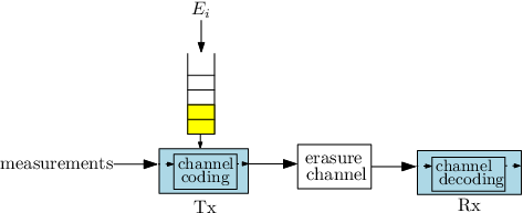
This paper is closely related to [35], in which coded status updates are proposed in order to overcome channel errors. We consider a single-user channel shown in Fig. 1, where the transmitter is energy harvesting and further transmission errors may occur due to energy outages. We consider two different types of channel codes to encode the status updates. First, we consider maximum distance separable (MDS) codes. With MDS coding, the transmitter encodes the status update symbols into symbols. The receiver receives the update successfully if it receives any of these encoded symbols. Next, we consider rateless codes, for example, fountain codes. In this case, the transmitter encodes the update symbols into as many symbols as needed until of these symbols are received successfully. For each of these models, we consider two different policies: best-effort and save-and-transmit. Best-effort and save-and-transmit schemes were originally considered in [41], in the context of achieving the capacity of the energy harvesting AWGN channel. In the best-effort scheme, in each slot, the transmitted symbol may suffer from two errors: channel erasure and energy outage. In the save-and-transmit scheme, the transmitter remains silent at the beginning to save energy and to reduce the errors due to energy outage.
For all these cases, we derive the average AoI. Through numerical results, we show that as the average recharge rate decreases, MDS codes with save-and-transmit outperforms all the best-effort schemes. The gain becomes significant for low values of average energy arrivals. We observe that rateless coding with save-and-transmit outperforms all other policies.
II System Model
We consider a single-user channel with a transmitter which has an infinite-sized battery, see Fig. 1. The energy arrivals are Bernoulli and i.i.d.: in slot , a unit energy arrives with probability or no energy arrives with probability , i.e., . The transmitter obtains the measurements (status updates), which are packets of length , which should be sent to the receiver in a way to minimize the average AoI at the receiver.
The total AoI up to time is,
| (1) |
where is the time stamp of the latest received status update packet and is the instantaneous AoI.
An example evolution of the AoI is shown in Fig. 2. The average long-term AoI in this case is calculated as,
| (2) |
In all the subsequent analysis we will assume renewal policies, i.e., where and are i.i.d. The AoI then reduces to,
| (3) |
where we dropped the subscript as and are i.i.d.
The channel between the transmitter and the receiver is an i.i.d. erasure channel. The probability of symbol erasure (loss) in each slot is . In order to combat the channel erasures and the energy outages, the transmitter encodes the status updates before sending them through the channel.
We consider two types of channel codes: MDS and rateless codes. We first consider MDS channel codes. For this case we have an channel coding scheme, where is the length of an uncoded status update and is the length of an encoded codeword which is sent through the channel with . When the transmitter is done with sending the symbols, it generates a new update and begins sending it. This is irrespective of the success of the transmission of these symbols. The optimal value of depends on , , and . For MDS channel coding, we study two achievable schemes. We first study a save-and-transmit scheme in which the transmitter saves energy from the incoming energy arrivals until it has at least units of energy in its battery. This in effect makes sure that errors which can occur during the codeword transmission are only due to the erasures in the channel. To ensure that the synchronization is maintained between the transmitter and the receiver, the transmitter remains in the saving phase for a number of slots which is multiple of . We then study a best-effort scheme, in which the transmitter attempts transmission in each slot. In this case, the error in each symbol can be either due to an energy outage or a channel erasure or both.
We next study the case of rateless coding in which the transmitter keeps sending the update until symbols are successfully received. For this case, we also study two schemes: best-effort and save-and-transmit. In the best-effort scheme, once the update is successfully received, the transmitter generates a new update and begins transmitting it immediately. In the save-and-transmit scheme, once the update is successfully received, the transmitter waits some time in order to save some energy in the battery to prevent future energy outages. The transmitter saves for slots, where the optimal should be obtained as a function of the system parameters , , and .

III AoI Under MDS Channel Coding
III-A Save-and-Transmit Policy
In the save-and-transmit policy, before the transmitter attempts to transmit the coded update, the transmitter remains silent for an integer multiple of slots until the battery has energy at least equal to . The duration the transmitter remains silent for the th time while transmitting the th update is a random variable denoted by which depends on the energy arrival distribution. The random variable can be expressed as:
| (4) |
where is the random variable which denotes the number of slots needed to save units of energy and denotes the smallest integer greater than or equal to . Since the energy arrivals follow an i.i.d. Bernoulli distribution, will follow a negative binomial distribution as follows:
| (5) |
The distribution of can be obtained using (5) as follows:
| (6) |
After the saving phase, the transmission resumes for slots. After the transmitter is done transmitting the coded symbols, the transmitter again goes to the saving phase until it recharges its battery to at least . The transmitter alternates between saving and transmission phases.
The update is successful if at least symbols are received without being erased; there will be no energy outage due to the saving phase. Hence, the probability of having a success in a slot of duration is,
| (7) |
Thus, in the consecutive slots the transmission is successful with probability . Now, the update will be successful in the th transmission, where is a geometrically distributed random variable with a the following pmf,
| (8) |
Hence, we may need to repeat the save-and-transmit phases for times before we have a successful status update.
We now characterize the random variable which identifies the instant at which the update will be successful within the consecutive slots. We denote this random variable by which has a conditional pmf where
| (9) |
Hence, is distributed as:
| (10) |
An example which illustrates the AoI evolution is shown in Fig. 3. In this figure, the transmitter at first waits slots in order to recharge the battery to at least the level . It then attempts to transmit. The transmission in this case is not successful due to the channel erasures so the transmitter again waits for slots in order to charge the battery. The transmission then proceeds again in the next slot. The transmission is then successful and the receiver received the update after transmissions, where .

We now consider a renewal policy which serves as an upper bound for the save-and-transmit policy described above. We assume that at the end of the update period, the transmitter depletes all its battery. Thus, the transmitter renews its state at the end of each successful update and always begins with a depleted battery. In this case, the AoI can be written as:
| (11) |
Next, we evaluate and . We first obtain as,
| (12) | ||||
| (13) |
We then obtain as,
| (14) |
Now, it remains to calculate the expectation of and . We first calculate the first and second moments of , using [42, Theorem 6.13], as follows:
| (15) |
Similarly, we have:
| (16) |
We then combine all these to obtain:
| (17) |
and
| (18) |
where and can be calculated using (6) and can be calculated using (10). Hence, the average AoI in (11) can be found by substituting with the expressions in (17) and (18).
III-B Best-Effort Policy
We now consider the case when the transmitter does not wait at the beginning in order to save energy, instead it begins transmission immediately. The error events in this case can be either an erasure in the communication channel or an energy outage at the transmitter. These two events may occur for each transmitted symbol. Hence, for the symbol to be received without an error, there should be no energy outage and no channel erasure; this forms a Bernoulli random variable with probability of success equal to . The evolution of AoI is similar to Fig. 3 but in this case, is equal to zero as the transmitter does not wait to save energy.
Using analysis similar to the previous scheme, but with having the probability of success equal to , the average AoI in this case can be written as:
| (19) |
This can also be obtained using the same analysis as in [35], but with probability of success equal to ,
IV AoI Under Rateless Channel Coding
IV-A Best-Effort Policy
We consider here the case when the transmitter begins to transmit immediately. In each slot, the transmitter suffers two possible error events. The first is channel erasure and the second is energy outage. Hence, a symbol will be received successfully if neither error occurs, which happens with probability equal to . The channel is now equivalent to an erasure channel, similar to the one considered in [35], but with probability of success equal to . Following analysis similar to the one in [35], but with probability of success equal to , the average AoI in this case is equal to:
| (20) |

IV-B Save-and-Transmit Policy
In this policy, we consider the case when the transmitter does not generate a new update immediately once the transmission of the previous update is successful, but it waits for a deterministic time of slots. Here, is a deterministic number which both the transmitter and the receiver know in advance; this should then be optimized to minimize the average AoI and will be a function of , and .
The transmission in this policy proceeds as follows: once the previous update is successful, the transmitter begins a saving phase of duration slots. Then, the transmitter generates a new update and begins transmitting it to the receiver. While transmitting the update, the transmitter may receive more energy arrivals; however, the amount of energy in the battery will always be non-increasing as the transmitter transmits a symbol in each slot while the energy may not arrive at every slot. The transmitter keeps transmitting the update until its battery state hits zero; this declares the end of the no-outage phase. We denote the number of symbols sent successfully in this phase by . If , then no more transmission is required and the update is successful. Otherwise, the transmitter transmits the remaining using the best-effort scheme described in Subsection IV-A.
We denote the duration the transmitter transmits with no outage by and we denote the duration we transmit using the best-effort scheme by . An example for the evolution of the AoI in this case is shown in Fig. 4. The average AoI can be calculate as follows,
| (21) | ||||
| (22) |
This AoI can be calculated explicitly once , , , and are calculated. We note that and are dependent on each other while and are independent due to using a renewal policy.
We now define the random variables ; the random variable represents the amount of energy harvested in the first slots. For , the random variable represents the amount of energy harvested during the previous slots. Hence, we have .
We now characterize the random variable ,
| (23) |
where is Bin, and for , given is Bin; Bin denotes binomial distribution. An example for the evolution of is shown in Fig. 5.

We can obtain the marginal pmf for the random variables , , by applying [42, Theorem 6.12] and using [42, Table 6.1]. Each consists of a sum of i.i.d. Bernoulli random variables and the number of these random variables is distributed according to a binomial distribution of which is independent of the Bernoulli random variables. Hence, the marginal pmf of the random variable is Bin(,).
We can now calculate as,
| (24) |
Next, we want to calculate which we calculate as . The term can be calculated as follows
| (25) | ||||
| (26) |
This requires the calculation of , . To calculate the covariance, we first calculate the conditional probability . For , we have that is distributed as Bin(,). This again follows by applying [42, Theorem 6.12] and using [42, Table 6.1].
We now calculate for as follows:
| (27) |
Next, we calculate as follows:
| (28) | ||||
| (29) |
Therefore, is equal to
| (30) |
Hence, can be calculated as follows:
| (31) |
Next, we calculate , and . The pmf of is negative binomial distribution as in (5) but with number of successes equal to and with success probability equal to . The value of can then be calculated using conditional expectation as follows:
| (32) |
and the value of can be calculated as follows
| (33) |
where . Similarly, we can obtain . Now, it remains to calculate the expectation over the pmf of . Due to the dependency between the terms and their infinite sum, there is no closed form for the pmf of and it can be found numerically.


V Numerical results
In this section, we compare the performances of the proposed schemes. When there is no energy harvesting, i.e., energy arrives with probability at every slot, rateless coding has the best AoI (this mimics the result obtained in [35]) and save-and-transmit with MDS coding has the worst performance. The reason that the save-and-transmit with MDS coding has the worst performance is that it requires a saving phase of at least slots, which is not necessary as the energy arrives at all slots. When the probability of energy arrivals decreases to , save-and-transmit with MDS coding performs the same as the best-effort rateless coding case, as shown in Fig. 7. Rateless coding with save-and-transmit performs slightly better than all the other policies. As the probability of energy arrival decreases further, save-and-transmit with MDS coding outperforms all the best-effort policies as shown in Fig. 8 and Fig. 9. As shown in Fig. 9, the gain becomes significant for low values of . The reason for this is that save-and-transmit eliminates the errors due to energy outage by saving sufficient energy before attempting to transmit. For example, in Fig. 9, for the best-effort scheme, the probability of success in transmitting a symbol is equal to , while if we eliminate the energy outage due to energy harvesting as in save-and-transmit scheme, the success probability for reach symbol will be , which is much higher than the best-effort scheme. Rateless coding with save-and-transmit is better than MDS coding with save-and-transmit, because rateless coding with save-and-transmit gives more flexibility for the transmitter to choose just the right saving duration, while in MDS coding case, the transmitter is forced to save for a multiple of slots.


References
- [1] J. Yang and S. Ulukus. Optimal packet scheduling in an energy harvesting communication system. IEEE Trans. Comm., 60(1):220–230, January 2012.
- [2] K. Tutuncuoglu and A. Yener. Optimum transmission policies for battery limited energy harvesting nodes. IEEE Trans. Wireless Comm., 11(3):1180–1189, March 2012.
- [3] O. Ozel, K. Tutuncuoglu, J. Yang, S. Ulukus, and A. Yener. Transmission with energy harvesting nodes in fading wireless channels: Optimal policies. IEEE JSAC, 29(8):1732–1743, September 2011.
- [4] C. K. Ho and R. Zhang. Optimal energy allocation for wireless communications with energy harvesting constraints. IEEE Trans. Signal Proc., 60(9):4808–4818, September 2012.
- [5] J. Yang, O. Ozel, and S. Ulukus. Broadcasting with an energy harvesting rechargeable transmitter. IEEE Trans. Wireless Comm., 11(2):571–583, February 2012.
- [6] J. Yang and S. Ulukus. Optimal packet scheduling in a multiple access channel with energy harvesting transmitters. Journal of Comm. and Networks, 14(2):140–150, April 2012.
- [7] Z. Wang, V. Aggarwal, and X. Wang. Iterative dynamic water-filling for fading multiple-access channels with energy harvesting. IEEE JSAC, 33(3):382–395, March 2015.
- [8] O. Orhan and E. Erkip. Energy harvesting two-hop communication networks. IEEE JSAC, 33(12):2658–2670, November 2015.
- [9] B. Gurakan and S. Ulukus. Cooperative diamond channel with energy harvesting nodes. IEEE JSAC, 34(5):1604–1617, May 2016.
- [10] D. Gunduz and B. Devillers. Two-hop communication with energy harvesting. In IEEE CAMSAP, December 2011.
- [11] B. Varan and A. Yener. Delay constrained energy harvesting networks with limited energy and data storage. IEEE JSAC, 34(5):1550–1564, May 2016.
- [12] A. Arafa, A. Baknina, and S. Ulukus. Energy harvesting two-way channels with decoding and processing costs. IEEE Trans. on Green Comm. and Networking, 1(1):3–16, March 2017.
- [13] D. Gunduz and B. Devillers. A general ramework for the optimization of energy harvesting communication systems with battery imperfections. Journal of Comm. Networks, 14(2):130–139, April 2012.
- [14] O. Orhan, D. Gunduz, and E. Erkip. Energy harvesting broadband communication systems with processing energy cost. IEEE Trans. Wireless Comm., 13(11):6095–6107, November 2014.
- [15] J. Xu and R. Zhang. Throughput optimal policies for energy harvesting wireless transmitters with non-ideal circuit power. IEEE JSAC, 32(2):322–332, February 2014.
- [16] O. Ozel, K. Shahzad, and S. Ulukus. Optimal energy allocation for energy harvesting transmitters with hybrid energy storage and processing cost. IEEE Trans. Signal Proc., 62(12):3232–3245, June 2014.
- [17] K. Tutuncuoglu, A. Yener, and S. Ulukus. Optimum policies for an energy harvesting transmitter under energy storage losses. IEEE JSAC, 33(3):476–481, March 2015.
- [18] H. Mahdavi-Doost and R. Yates. Energy harvesting receivers: Finite battery capacity. In IEEE ISIT, July 2013.
- [19] R. Yates and H. Mahdavi-Doost. Energy harvesting receivers: Optimal sampling and decoding policies. In IEEE GlobalSIP, December 2013.
- [20] H. Mahdavi-Doost and R. Yates. Fading channels in energy-harvesting receivers. In CISS, March 2014.
- [21] J. Rubio, A. Pascual-Iserte, and M. Payaro. Energy-efficient resource allocation techniques for battery management with energy harvesting nodes: a practical approach. In Euro. Wireless Conf., April 2013.
- [22] A. Arafa and S. Ulukus. Optimal policies for wireless networks with energy harvesting transmitters and receivers: Effects of decoding costs. IEEE JSAC, 33(12):2611–2625, December 2015.
- [23] O. Ozel, S. Ulukus, and P. Grover. Energy harvesting transmitters that heat up: Throughput maximization under temperature constraints. IEEE Wireless Comm., 15(8):5440–5452, August 2016.
- [24] A. Baknina, O. Ozel, and S. Ulukus. Energy harvesting communications under temperature constraints. In UCSD ITA, February 2016.
- [25] A. Baknina, O. Ozel, and S. Ulukus. Explicit and implicit temperature constraints in energy harvesting communications. In IEEE Globecom, December 2017.
- [26] S. Kaul, R. Yates, and M. Gruteser. Real-time status: How often should one update? In IEEE INFOCOM, March 2012.
- [27] S. Kaul, R. Yates, and M. Gruteser. Status updates through queues. In CISS, March 2012.
- [28] R. Yates and S. Kaul. Real-time status updating: Multiple sources. In IEEE ISIT, July 2012.
- [29] C. Kam, S. Kompella, and A. Ephremides. Age of information under random updates. In IEEE ISIT, July 2013.
- [30] M. Costa, M. Codreanu, and A. Ephremides. Age of information with packet management. In IEEE ISIT, June 2014.
- [31] Y. Sun, E. Uysal-Biyikoglu, R. Yates, C. E. Koksal, and N. B. Shroff. Update or wait: How to keep your data fresh. In IEEE INFOCOM, April 2016.
- [32] A. Kosta, N. Pappas, A. Ephremides, and V. Angelakis. Age and value of information: Non-linear age case. Available at arXiv:1701.06927.
- [33] A. M. Bedewy, Y. Sun, and N. B. Shroff. Age-optimal information updates in multihop networks. Available at arXiv:1701.05711, 2017.
- [34] P. Parag, A. Taghavi, and J. Chamberland. On real-time status updates over symbol erasure channels. In IEEE WCNC, pages 1–6, March 2017.
- [35] R. Yates, E. Najm, E. Soljanin, and J. Zhong. Timely updates over an erasure channel. In IEEE ISIT, June 2017.
- [36] R. Yates. Lazy is timely: Status updates by an energy harvesting source. In IEEE ISIT, June 2015.
- [37] B. T. Bacinoglu, E. T. Ceran, and E. Uysal-Biyikoglu. Age of information under energy replenishment constraints. In USCD ITA, February 2015.
- [38] X. Wu, J. Yang, and J. Wu. Optimal status update for age of information minimization with an energy harvesting source. Available at arXiv:1706.05773, 2017.
- [39] A. Arafa and S. Ulukus. Age minimization in energy harvesting communications: Energy-controlled delays. In IEEE Asilomar, October 2017.
- [40] A. Arafa and S. Ulukus. Age-minimal transmission in energy harvesting two-hop networks. In IEEE Globecom, December 2017.
- [41] O. Ozel and S.Ulukus. Achieving AWGN capacity under stochastic energy harvesting. IEEE Trans. Info. Theory, 58(10):6471–6483, October 2012.
- [42] R. Yates and D. Goodman. Probability and Stochastic Processes, 2nd ed.