Dominance analysis of linear complementarity systems
Abstract
The paper extends the concepts of dominance and -dissipativity to the non-smooth family of linear complementarity systems. Dominance generalizes incremental stability whereas -dissipativity generalizes incremental passivity. The generalization aims at an interconnection theory for the design and analysis of switching and oscillatory systems. The approach is illustrated by a detailed study of classical electrical circuits that switch and oscillate.
I INTRODUCTION
Dominance analysis and p-dissipativity were recently introduced in [1, 2] to extend the application of dissipativity theory to the analysis of multistable and oscillatory systems. The approach is differential, that is, based on the analysis of linearized dynamics along trajectories, in the spirit of contraction theory [3], convergence analysis [4], or differential stability analysis [5]. It is particularly adapted to systems whose linearization can be easily parametrized, such as Lure systems that interconnect linear time-invariant systems with static nonlinearities [6]. The present paper investigates how to extend this analysis to nonlinear circuits modeled as linear complementarity systems: models that consist of linear time-invariant systems augmented with a static complementarity constraint. The modeling framework of linear complementarity systems has proven very useful to analyze systems whose nonlinear dynamical behavior arises from non-smooth constraints [7, 8, 9, 10, 11]. They find applications in a number of fields including mechanical systems with unilateral constraints [12], electrical circuits with diodes [13], and mathematical programming [14]. Linear complementarity systems provide an attractive framework for dominance analysis because they are general enough to model switching and oscillatory behaviors often encountered in the presence of non-smooth constraints and specific enough to lead to tractable analysis. In particular, the passivity property of complementarity constraints has proven central to analyze linear complementarity systems in the framework of dissipativity theory [15, 9]. Linear complementarity systems hence offer an ideal platform for the application of -dissipativity theory to switching and oscillatory behaviors. To account for the non-smoothness of linear complementarity systems, the differential analysis of [1, 2] has to be replaced by incremental analysis [16], [17], [18]. Incremental analysis studies how increments between trajectories evolve in time, whereas differential analysis only considers linearized trajectories, that it, infinitesimal increments. In the context of linear complementarity systems, the difference is technical rather than conceptual. We show that the main results of [1, 2] extend to the incremental setting imposed by non-smooth constraints. This paper is organized as follows. In Section II we briefly review the modeling of linear complementarity systems and its core passivity property. Section III is dedicated to the property of dominance and -dissipativeness in the incremental setting. The example Section IV illustrates the potential of -dissipativity theory to analyze classical switching and oscillatory circuits. The papers ends with conclusions in Section V.
II Linear complementarity systems and incremental passivity
II-A Linear complementarity systems
A linear complementarity system [15] consists of a linear dynamical system subject to a complementarity constraint
| (1) |
where is the state variable, and are the so-called complementary variables, and is an additional control input. The matrices , and are constant and of the appropriate dimensions. The complementarity condition is a compact representation of the following three conditions: i) , ii) , and iii) . A solution of the linear complementarity system (1) is any tuple such that is an absolutely continuous function and satisfies (1) for almost all forward times . In general, we assume that the initial conditions are such that the complementarity conditions hold. This implies the absence of jumps in the initial condition and in the complementarity variables [9].
II-B Incremental passivity
A cornerstone in the analysis of linear complementarity systems is to observe that the complementarity relation
| (2) |
defines an incrementally passive relation. We recall the definition and the proof of that property.
Definition 1
A relation is incrementally passive if for any , and any the inequality
| (3) |
holds.
Proposition 2
is incrementally passive.
Proof:
Take and . Then, .
∎An alternative description of the relation is via the multivalued map
| (4) |
which leads to the feedback representation in Figure 1.
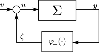
This Lure type representation of linear complementarity systems calls for an analysis rooted in passivity theory: the linear complementary system is incrementally passive as the negative feedback interconnection of a linear passive system with an incrementally passive relation. Passivity of the linear part is a standard assumption in the literature on linear complementarity systems; it guarantees existence and uniqueness of solutions for (1). Details can be found in [9], [8], [19] based on the following additional assumption, which ensures well-posedness of the closed loop in the presence of the throughput term , [9].
Assumption 3
The linear part of (1) is a minimal realization, it is passive and the matrix
| (5) |
has full column rank.
Passivity of the linear part of (1) from to reads
| (6) |
where the derivative of the quadratic storage , , is computed along the linear dynamics. Passivity and incremental passivity coincide for linear systems. In fact, for any pair of trajectories , outputs and inputs , the incremental dynamics characterized by the variables , , satisfies
| (7) |
Since the negative feedback interconnection of incrementally passive systems is incrementally passive [15], the closed loop linear complementarity system is incrementally passive. For any constant input , the resulting closed loop is thus incrementally stable, that is, there exists a nondecreasing function such that
for any pair of trajectories , of (1). Furthermore, if the passive inequality (6) is strict, the resulting closed loop becomes incrementally asymptotically stable; its trajectories converge towards each other
In this case, an equilibrium point is necessarily unique and globally stable. The concept of incremental stability [20] is analog to the concept of differential stability in the theory of contraction [3] or convergent systems [4]. But it does not require any differentiability of the system dynamics.
II-C Beyond linear complementarity relations
For the purpose of this paper, the linear complementarity condition can be replaced by any incrementally passive static relation. Figure 2 provides an illustration of incrementally passive memoryless nonlinearities. Those multivalued maps are widely used for modeling electronic circuits. For example, the three graphs in Figure 2 represent the ideal current-voltage characteristic of a diode, of a zener diode, and of an array of diodes [21], [22].

Denoting any pair that belongs to the -th relation in Figure 2, we extend the class of linear complementarity systems to the family of systems of the form
| (8) |
Following the approach of linear complementarity systems, for a solution of (8) we mean any tuple such that is an absolutely continuous function and satisfies (8) for almost all forward times . Indeed, the closed loop (8) allows for the block diagram representation in Figure 1, with replaced by , the static multivalued map associated to the relation . Thus, for any passive relation , the closed loop (8) is incrementally passive. We remark that incremental passivity guarantees existence and uniqueness of solutions also for general maximal monotone static multi-valued maps, [8].
III Dominance and -dissipativity
III-A Dominance
Dominance was recently introduced in [1], [2], [6] as a generalization of incremental stability for smooth nonlinear systems. Motivated by dominance analysis of linear complementarity systems, we extend the definition of dominance in a nonsmooth setting, replacing differential analysis by incremental analysis as in the previous section. For the sake of simplicity in this section, and the rest of the paper, we consider generic pairs of trajectories and , and we adopt the notation to denote their mismatch. is defined for almost every by the right-hand side of (8) computed for and , respectively. A similar notation is adopted for inputs and outputs . Finally, we say that a symmetric matrix has inertia when it has negative eigenvalues and positive eigenvalues.
Definition 4
Note that dominance is just incremental stability if is positive definite, which corresponds to . But we are interested in the generalization corresponding to and to . For smooth closed systems , (9) is equivalent to the linear matrix inequality inequality
| (10) |
where denotes the Jacobian of at . In the linear case, , (10) implies the existence of an invariant splitting such that , where is the -dimensional eigenspace associated to the dominant modes of (eigenvalues of whose real part is larger than ), and is the -dimensional eigenspace associated to the transient modes of (i.e., the eigenvalues of whose real part is smaller than ). Roughly speaking, in the nonlinear case the property of dominance forces the asymptotic behavior to be -dimensional [2, Theorem 2], as shown by the analysis of the linearized flow in [2, Theorem 1]. The following theorem extends [2, Theorem 2] to the nonsmooth case.
Theorem 5
Proof:
Consider any pair of trajectories and , define the increment , and consider the quadratic form . From (9),
therefore
By integration,
| (11) |
Let and be two different points of and define . Note that both and are accumulation points of a suitable trajectory, therefore and (11) implies
| (12) |
Let , be the eigenspaces of associated to the negative eigenvalues of , and positive eigenvalues of , respectively. Let be the projection onto along . We claim that restricted to is one-to-one. In fact, assume by contradiction that for , implies , it follows that and therefore which contradicts (12). Hence, restricted to is one-to-one.
Now, for each constant input , consider the equivalent representation of the system (8) based on the differential inclusion
| (13) |
Using the results above, if then there exists a unique initial condition such that and the flow in is generated by the vector field
| (14) |
which is -dimensional. ∎Theorem 5 shows that the asymptotic behavior of a strict -dominant system is strongly constrained for small values of .
Corollary 6
Let the assumptions of Theorem 5 hold. In addition, assume that solutions of (8) are unique. Then all solutions asymptotically converge to
- 1.
a unique equilibrium point, if .
- 2.
an equilibrium point, if .
- 3.
an equilibrium point, a set of equilibrium points and connecting arcs, or a limit cycle, if .
Under uniqueness of solutions, distinct trajectories cannot intersect. For , the asymptotic dynamics are one-dimensional, forcing bounded trajectories to converge to some fixed point. Uniqueness of solutions is also sufficient for guaranteeing the validity of the Poincaré-Bendixson Theorem, see e.g., [23, Theorem 5.3]. Hence, under the assumption of uniqueness of solutions, a -dominant system with a compact limit set that contains no equilibrium point has a closed orbit.
III-B Incremental -dissipativity
Dissipativity theory is an interconnection theory for stability analysis. In the same way, -dissipativity is an interconnection theory for dominance analysis [2], [6]. It mimics standard dissipativity theory in the differential/incremental setting but relies on quadratic storage functions that have a prescribed inertia.
Definition 7
A nonsmooth system (8) is -dissipative with rate and incremental supply
| (15) |
if there exists a matrix with inertia and such that
| (16) |
for any pair of trajectories. Strict -dissipativity holds for .
-dissipativity coincides with the classical concept of incremental dissipativity. -dissipativity allows for an interconnection theory for non-smooth systems, as clarified by the next theorem. The simplest example is given by the closed loop in Figure 1.
Theorem 8
Let and be (strict) and dissipative respectively, both with rate and supplies
The negative feedback interconnection
of and is (strict) -dissipative with respect to the input and the output , with incremental supply given by
and rate . In addition, if
then the interconnection is (strictly) -dominant.
Proof:
The proof follows by standard arguments of dissipativity theory. See also [1]. ∎Classical dissipativity theory provides a tool to analyze stable systems, that is, -dominant systems, as interconnection of dissipative open systems, that is, -dissipative systems. Theorem 8 generalizes this conclusion: -dominant systems can be analyzed as interconnections of -dissipative systems with a -dissipative system; -dominant systems can be analyzed as interconnections of -dissipative systems with a -dissipative system, or as interconnections of two -dissipative systems.
III-C -Passivity of linear complementarity systems
As in the classical theory, -passivity is -dissipativity for the particular supply rate
| (17) |
We have seen in Section II that the linear complementarity relation is -passive (since -passivity and incremental passivity coincide). Also the static nonlinearities in Section II-C are -passive. Thus, from Theorem 8, the non-smooth system (8) is the negative feedback loop of a -passive static nonlinearity with a linear system, whose degree of -passivity determines the degree of passivity of the closed loop. The degree of passivity of the linear part restricts the asymptotic behavior of the system. We observe that for linear systems of the form , , the inequality (16) with (17) reduces to the simple feasibility test
for some matrix with inertia ; a numerically tractable condition. Also, -passivity has a frequency domain characterization based on the rate-shifted transfer function , [6]:
Proposition 9
A linear system is -passive if and only if the following two conditions hold,
- 1.
, for all, .
- 2.
has poles on the right-hand side of the complex plane.
Frequency domain conditions prove useful in capturing the limits of the theory and for the selection of the systems parameters, as shown in the next section.
IV Switching and oscillating LCS circuits
IV-A The operational amplifier is -passive
A model of the operational amplifier is shown in Figure 3: a first order model [24], with additional voltage saturation limits, implemented via ideal diodes, to take into account the physical limitations of any op-amp device. Note that the right-most element in the model denotes a buffer, which decouples the output current from the internal circuit. We make the usual assumption of infinite input impedance and output impedance .

The model in Figure 3 is described by the linear complementarity system
| (18a) | ||||
| (18b) | ||||
| (18c) | ||||
| (18d) | ||||
where we assume that the voltage sources and are constant and , . The model is derived via Kirchhoff’s laws together with the complementarity conditions for the diodes [21]. denotes the voltage across the capacitor . The input is set to and the output is . For completeness, we write (18) in the standard linear complementarity form (1) by taking , , , ,
A representation of (18) is the negative feedback interconnection of a strictly -passive system with a -passive relation defined by (18b),(18c), and (18d), linking voltage and the difference of diode currents . The relations and imply . Thus, the output of the op-amp always belongs to the interval . For , (18c) and (18d) imply that and , respectively, that is, . Similarly, implies and implies . Hence, corresponds to the -passive relation represented in Figure 2.ii). Its associated multivalued function maps the voltage into
The operational amplifier model (18) is thus given by the feedback loop in Figure 4, combining the -passive linear system with matrices , , and , with the -passive nonlinearity . The transfer function of reads
| (19) |
and Proposition 9 guarantees strict -passivity with rate . By Theorem 8, the op-amp is thus a strictly -passive device from to with rate .

IV-B Positive feedback amplifier: multistable Schmitt trigger
The positive feedback interconnection of the op-amp with an additional passive network leads to -passive circuits. For instance, the Schmitt trigger circuit represented in Figure 5 contains an op-amp, whose model is given by (18), and a linear network represented by
| (20) |
where is the voltage across the capacitor .

Their interconnection is characterized by the positive feedback identity
| (21) |
Positive feedback loops of two -passive systems are not -passive. But is also strictly -passive from the input to the output with rate , which allows to rewrite (21) as negative feedback
| (22) |
Indeed, the positive feedback in (21) is equivalent to the negative feedback between a strictly -passive system, the op-amp, and a strictly -passive system, . Thus, by selecting the circuit parameters to satisfy
| (23) |
Theorem 8 guarantees that the Schmitt trigger is strictly -passive with rate . The closed loop is thus strictly -dominant. An interpretation of (23) is that the linear circuit must have a slower dynamics than the op-amp dynamics, to determine a dominant behavior of dimension . Mathematically, (23) guarantees the existence of a common rate for which op-amp and are respectively -passive and -passive, as required by Theorem 8. A -passive circuit can be multistable. Bounded trajectories of a strictly -dominant system necessarily converge to a fixed point. Boundedness of trajectories follows from the saturation of the op-amp voltage, which essentially “opens the loop” for large overshoots. To enforce multistability, we look for circuit parameters that guarantee the existence of at least one unstable equilibrium point. The condition
| (24) |
makes the zero-equilibrium unstable. The parameters in Table I satisfies (23) and (24), enabling bistability. The value of resistance and capacitance have been taken from [24], to ensure good matching between simulations and the behavior of a real op-amp component. Figure 6 shows the trajectories of the system from two different initial conditions .

IV-C Mixed feedback amplifier: relaxation oscillator
The interconnection of the op-amp with two slow passive networks, one with negative and one with positive feedback, leads to -passive circuits. For instance, the circuit in Figure 7 is a typical architecture for the generation of relaxation oscillations. It is derived from the Schmitt trigger through the addition of a slow network , in negative feedback, represented by
| (25) |
where is the voltage across the capacitor .

The interconnection of the op-amp and of the two networks and is given by the mixed positive/negative feedback
| (26) |
which can be written as a standard negative feedback loop using the aggregate output , for instance
| (27) |
Taking , , and , the aggregate transfer function from to reads
| (28) |
For , there is no negative feedback and the system reduces to the Schmitt trigger. For , the negative feedback loop either stabilizes the closed loop system, typically for parameter values that guarantee -passivity of , or induces oscillations, typically for parameter values that guarantee -passivity of . For instance, has positive real part if
Hence, by Proposition 9, if
then is strictly -passive with rate . The overall closed loop has a globally asymptotically stable fixed point. In contrast, for
is strictly -passive with rate . Thus, by Theorem 8, the overall closed-loop is -dominant with rate . Indeed, divides the fast op-amp dynamics from the dominant two dimensional slow dynamics of the linear networks. We conclude the section with a numerical simulation. The parameters of Table I together with , and satisfy the conditions above, thus guarantee strict -dominance the closed loop with rate . The fixed point in is unstable but all trajectories remain bounded (the constraint implies that and remain bounded), which enforces oscillations, as shown in Figure 8.

V CONCLUSIONS
We extended the concept of dominance to the analysis of nonsmooth linear complementarity systems. The extension mimics the smooth case when uniqueness of solutions is assumed. The approach is based on the interconnection theory of dissipativity. It opens the way to the analysis of switching or oscillatory circuits with no restriction on the dimension of the state-space. The potential of the approach was illustrated with a detailed analysis of well-known circuits based on op-amps, predicting multistable and oscillatory behaviors, while providing margins on the circuit parameters to enable such behaviors.
References
- [1] F. Forni and R. Sepulchre, “A dissipativity theorem for -dominant systems,” in 56th IEEE Conference on Decision and Control, Melbourne, Australia, 2017.
- [2] ——, “Differential dissipativity theory for dominance analysis,” 2017, submitted to IEEE Transactions on Automatic Control, http://arxiv.org/abs/1710.01721.
- [3] W. Lohmiller and J.-J. E. Slotine, “On contraction analysis for nonlinear systems,” Automatica, vol. 34, no. 6, pp. 683–696, 1998.
- [4] A. Pavlov, N. Van De Wouw, and H. Nijmeijer, “Convergent systems: analysis and synthesis,” in Control and observer design for nonlinear finite and infinite dimensional systems. Springer, 2005, pp. 131–146.
- [5] F. Forni and R. Sepulchre, “A differential Lyapunov framework for contraction analysis,” IEEE Transactions on Automatic Control, vol. 59, no. 3, pp. 614–628, 2014.
- [6] F. A. Miranda-Villatoro, F. Forni, and R. Sepulchre, “Analysis of Lur’e dominant systems in the frequency domain,” 2017, submitted to Automatica, http://arxiv.org/abs/1710.01645.
- [7] B. Brogliato, “On the control of non-smooth complementarity dynamical systems,” Philosophical Transactions of the Royal Society of London. Series A: Mathematical, Physical and Engineering Sciences, vol. 359, no. 1789, pp. 2369–2383, 2001.
- [8] ——, “Some perspectives on the analysis and control of complementarity systems,” IEEE Transactions on Automatic Control, vol. 48, no. 6, pp. 918–935, 2003.
- [9] M. K. Çamlıbel, W. Heemels, and J. Schumacher, “On linear passive complementarity systems,” European Journal of Control, vol. 8, no. 3, pp. 220–237, 2002.
- [10] M. K. Çamlıbel, P. J. S, and J. L. Shen, “Lyapunov stability of linear complementarity systems,” SIAM Journal on Optimization, vol. 17, no. 4, pp. 1056–1101, 2006.
- [11] W. Heemels and B. Brogliato, “The complementarity class of hybrid dynamical systems,” European Journal of Control, vol. 9, no. 2, pp. 322–360, 2003.
- [12] B. Brogliato, Nonsmooth Mechanics, ser. Communications and Control Engineering. Springer, 2016.
- [13] V. Acary, O. Bonnefon, and B. Brogliato, Nonsmooth modeling and simulation for switched circuits, ser. Lecture Notes in Electrical Engineering. Springer, 2011.
- [14] A. Nagurney, Network economics: A variational inequality approach, ser. Advances in Computational Economics. Springer, 1999.
- [15] A. J. van der Schaft, L2-Gain and Passivity Techniques in Nonlinear Control, ser. Lecture Notes in Control and Information Sciences. Springer, 1996.
- [16] G. B. Stan and R. Sepulchre, “Analysis of interconnected oscillators by dissipativity theory,” IEEE Transactions on Automatic Control, vol. 52, no. 2, pp. 256–270, 2007.
- [17] A. Pavlov and M. L, “Incremental passivity and output regulation,” Systems & Control Letters, vol. 57, pp. 400–409, 2008.
- [18] T. Liu, D. J. Hill, and Z. J, “Incremental-dissipativity-based synchronization of interconnected systems,” in Proceeding of the 18th World Congress, Milano, Italy, 2011, pp. 8890–8895.
- [19] F. A. Miranda-Villatoro and F. Castaños, “Robust output regulation of strongly linear passive systems with multivalued maximally monotone controls,” IEEE Transactions on Automatic Control, vol. 62, no. 1, pp. 238–249, 2017.
- [20] D. Angeli, “A Lyapunov approach to incremental stability properties,” IEEE Transactions on Automatic Control, vol. 47, pp. 410–421, 2000.
- [21] V. Acary and B. Brogliato, “Implicit Euler numerical scheme and chattering-free implementation of sliding mode systems,” Systems & Control Letters, vol. 59, no. 5, pp. 284–293, 2010.
- [22] Y. J. Lootsma, A. J. van der Schaft, and M. K. Çamlıbel, “Uniqueness of solutions of linear relay systems,” Automatica, vol. 35, pp. 467–478, 1999.
- [23] K. Ciesielski, “The Poincaré-Bendixson theorems for two dimensional semiflows,” Topological Methods in Nonlinear Analysis, vol. 3, pp. 163–178, 1994.
- [24] J. Karki, “Effect of parasitic capacitance in op amp circuits,” Texas Instruments, Tech. Rep. SLOA013A, 2000.