Accelerated Variational Quantum Eigensolver

To analyse RFPE’s convergence, we analyse the expected posterior variance $r^{2}$ (i.e. the Bayes risk) for a normal prior $\phi\sim\mathcal{N}(\mu,\sigma^{2})$. The formula for $r^{2}$ can be derived from Ref. [17, Appendix B] as:

$$\mathbb{E}_{E}[\mathbb{V}[\phi|M,\theta;\mu,\sigma]]\equiv r^{2}(M,\theta;\mu,\sigma)\equiv r^{2}(M,\theta)\equiv r^{2}=\sigma^{2}(1-\frac{M^{2}\sigma^{2}\text{sin}^{2}(M(\mu-\theta))}{e^{M^{2}\sigma^{2}}-\cos^{2}(M(\mu-\theta))}).$$

(8)

Note that $r^{2}$ is bounded below by an envelope $s^{2}\coloneqq\sigma^{2}(1-M^{2}\sigma^{2}e^{-M^{2}\sigma^{2}})$. As a function of $M$, $s^{2}$ has minimiser:

$$M_{0}=\frac{1}{\sigma}.$$

(9)

But $M_{0}$ may be far away from the minimiser $M_{1}$ of $r^{2}$ due to rapid oscillations of $r^{2}$, as a function of $M$, above the envelope $s^{2}$. Fortunately, the frequency of these oscillations is controlled by $\theta$. This control is exactly the reason why Ref. [25] introduced $\theta$. Numerical simulations in Ref. [25, Appendix C] showed that the optimal $\theta\approx\mu\pm\sigma$ can effectively remove oscillations from $r^{2}$. This aligns $r^{2}$ with its envelope $s^{2}$, forcing $M_{1}$ closer to $M_{0}$.

Therefore, it makes sense to choose $(M=1/\sigma,\theta=\mu\pm\sigma)$ if we wish to minimise $r^{2}(M,\theta)$. However, Ref. [25] did not give intuition. To gain intuition, we found a simple heuristic argument for why it makes sense to choose $(M\propto 1/\sigma,\theta=\mu\pm\sigma)$ if we wish to minimise $r^{2}(M,\theta)$. We present our argument in the box below.

Therefore, we choose $\theta=\mu\pm\sigma$ and trial $M=a/\sigma$ with $a\in\mathbb{R}$ in Eqn. 8 to give:

$$r^{2}(\frac{a}{\sigma},\mu\pm\sigma)=\sigma^{2}(1-g(a)),$$

(13)

where $g:\mathbb{R}\rightarrow\mathbb{R}$ is defined by:

$$g(x)\coloneqq\frac{x^{2}\text{sin}^{2}(x)}{e^{x^{2}}-\text{cos}^{2}(x)}.$$

(14)

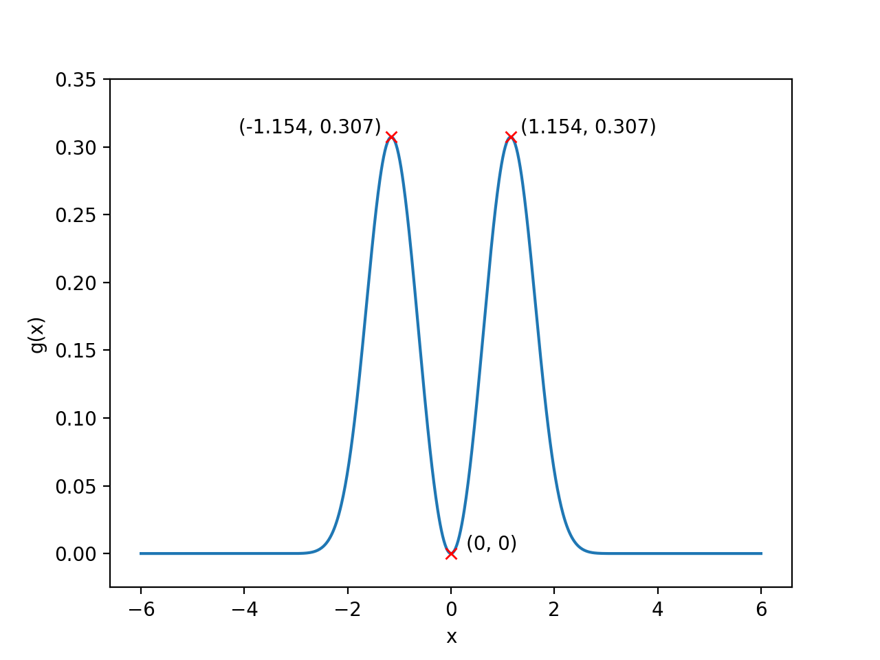
We find that $g$ has maximum value $g_{\text{max}}\approx 0.307$ at $x=\pm a_{0}$ where $a_{0}\approx 1.154$, and so $r^{2}$ has minimum value:

$$r_{\text{min}}^{2}=L^{2}\,\sigma^{2},$$

(15)

where $L^{2}\approx 0.693$. Therefore, after each iteration of RFPE, we expect the variance to (at least) decrease by a factor of $L^{2}$ when $M$ and $\theta$ are chosen optimally ⁴⁴ 4 Locally optimal $(M,\theta)$ at each iteration may not be globally optimal over a number of iterations. In fact, $A\approx 1.154$ differs from the globally optimal heuristic of $1.25$, but this distinction between local and global is besides the main point here and shall not be further discussed..

Writing $\sigma_{k}$ for the standard deviation at the $k$-th iteration, we rewrite Eqn. 15 as $\mathbb{E}[\sigma_{k}^{2}|\sigma_{k-1}^{2}]=L^{2}\,\sigma_{k-1}^{2}.$ Taking expectation over $\sigma_{k-1}$ gives $\mathbb{E}[\sigma_{k}^{2}]=L^{2}\,\mathbb{E}[\sigma_{k-1}^{2}]$. Assuming that $\mathbb{V}[\sigma_{k}]=0$ for $k$ large ⁵⁵ 5 We heuristically justify this and subsequent assumptions or approximations by good agreement of our final results Eqns. 25, 27 with numerical simulations., say $k\geq n_{0}$, we commute squaring with expectation to give $\mathbb{E}[\sigma_{k}]=L^{(k-k_{0})}\,\mathbb{E}[\sigma_{k_{0}}].$ Writing $r_{k}\coloneqq\mathbb{E}[\sigma_{k}]$ for the expected standard deviation at the $k$-th iteration gives:

$$r_{k}=L^{(k-k_{0})}\,r_{k_{0}},$$

(16)

so we expect the standard deviation to decrease exponentially with the number of iterations of RFPE.

Since $r_{k}$ of RFPE decreases exponentially with $k$, the use of $M\propto 1/\sigma_{k}$ at the $k$-th iteration means we expect $M$ to increase exponentially with $k$. This means that RFPE is indeed in the phase estimation regime which still has the same problem of requiring an exponentially long coherence time in the number of bits of precision required.

In the following, we address this problem by modifying the dependence of the $M$ on $\sigma$ at each iteration. We note that a possible additional restarting strategy in RFPE also addresses this same problem (see Appendix B) but for now, RFPE refers to RFPE without restarts.

Note that RFPE uses $M=O(1/\sigma)$ and is in the phase estimation regime, but if $M=O(1)$ at each iteration, we expect to recover the statistical sampling regime. We are led naturally then to consider $M$ of form:

$$M=a(\frac{1}{\sigma})^{\alpha},$$

(17)

with an introduced $\alpha\in[0,1]$ and some $a=a(\alpha)\in\mathbb{R}$ to facilitate a transition between the two regimes.

We again substitute $\theta=\mu\pm\sigma$, but $M$ as in Eqn. 17, into Eqn. 8, giving expected posterior variance:

$$r^{2}(a(\frac{1}{\sigma})^{\alpha},\mu\pm\sigma)=\sigma^{2}(1-g(b)),$$

(18)

where $b\coloneqq a\sigma^{(1-\alpha)}$ and $g$ remains defined by Eqn. 14. Ideally, we would like $b=a_{0}$ which gives $a=a_{0}(1/\sigma)^{(1-\alpha)},$ but we need $a$ to be independent of $\sigma$. From the graph of $g$ (Fig. 4), we see there is no natural way to define an optimal $a=a(\alpha)$ except when $\alpha=1$. So we could simply take $a=a_{0}$ (independent of $\alpha$) but instead we set $a=1$ for simplicity.

In the remainder of Appendix A, $\alpha\neq 1$ ($\alpha=1$ already analysed above) unless stated otherwise and we assume $r_{k}$ converges to zero. This is necessary for valid Taylor approximations and divisions by $(1-\alpha)$.

For $\sigma$ small, and so $b$ small, we have:

$$g(b)=\frac{b^{2}}{2}+O(b^{4}),$$

(19)

which we substitute into Eqn. 18 to give the following upon taking expectations and using the earlier assumption that $\mathbb{V}[\sigma_{k}]=0$ for $k$ large to commute the expectation:

$$r_{k+1}^{2}=r_{k}^{2}(1-\frac{1}{2}(r_{k}^{2})^{1-\alpha}),$$

(20)

which is similar to a logistic map in $r_{k}^{2}$. Taking log gives $\text{\text{log}}(r_{k+1}^{2})=\log(r_{k}^{2})-\frac{1}{2}r_{k}^{2(1-\alpha)},$ to $O(r_{k}^{4(1-\alpha)})$, which gives, upon writing $l_{k}=\text{log}(r_{k}^{2})$:

$$l_{k+1}=l_{k}-\frac{1}{2}e^{(1-\alpha)l_{k}}.$$

(21)

Assuming the existence of a differentiable function $l=l(t)$ with $l(t_{k})=l_{k}$ where $t_{k}\coloneqq nh$, we substitute $l$ into Eqn. 21 to obtain:

$$\frac{l(t_{k}+h)-l(t_{k})}{h}=\frac{-e^{(1-\alpha)l(t_{k})}}{2h}.$$

(22)

We further take $h$ small and assume LHS Eqn. 22 is well approximated by a derivative ⁶⁶ 6 This may be inconsistent with the previous assumption because it requires $l(t_{k}+h)-l(t_{k})\equiv l_{k+1}-l_{k}=O(h)$ and we assess its consequences in Eqn. 24.. Solving the resulting differential equation under initial condition at $(k_{0},r_{k_{0}})$ gives:

$$\text{log}(r_{k})=\text{log}(r_{k_{0}})-\frac{1}{2(1-\alpha)}\text{log}(1+r_{k_{0}}^{2(1-\alpha)}\frac{1-\alpha}{2}\,(k-k_{0})).$$

(23)

To assess Eqn. 23 with respect to the recurrence Eqn. 21 it intended to solve, we substitute it back to give:

$$l_{k+1}-l_{k}+\frac{1}{2}e^{(1-\alpha)l_{k}}=O((\frac{1}{(k-k_{0})^{2}+\frac{2}{1-\alpha}(1/r_{k_{0}}^{2})^{1-\alpha}})^{2}).$$

(24)

which we expect to equal zero. This means that for $k\geq k_{0}$, we expect Eqn. 23 to improve as a solution to Eqn. 21 as $k_{0}$ increases (and so $r_{k_{0}}$ decreases).

Given the considerable number of assumptions and approximations used to reach an analytical expression for the Bayes risk in Eqn. 23, one is justifiably cautious about its validity. For assurance, we plotted Eqn. 23 and Eqn. 16 (the latter for completeness but with $L^{2}$ reset to $L^{2}\approx 0.708$ corresponding to $a=1$) against numerical simulations of RFPE between iterations $0$ to $60$ with two initial conditions $(k_{0},r_{k_{0}})=(0,r_{0}\coloneqq 1)$ and $(20,r_{20})$. The numerical simulations are displayed in Fig. 5 and show good agreement with our analytical Eqn. 23 and Eqn. 16. Note that Eqn. 23 reduces to the form of Eqn. 16 in the $\alpha=1$ limit but not exactly because of the inaccuracy of approximation Eqn. 19 when $\alpha=1$. It is also essential to point out now that the Bayes risk is a measure of precision and not a priori a measure of accuracy (i.e. error). However, in Fig. 6, we numerically demonstrate that the median error aligns reasonably with the mean and median Bayes risk.

Having numerically addressed two potential caveats to Eqn. 23 in Fig. 5 and Fig. 6, we also observe from these Figures that Eqn. 23 is approximately valid for $(k_{0},r_{k_{0}})=(0,1)$. Assuming this validity, we rearrange Eqn. 23 to give:

$\displaystyle k$

$\displaystyle=f(r_{k},\alpha),$

(25)

where recall $f:\mathbb{R}\times[0,1]\rightarrow\mathbb{R}$ is the continuous function:

$$f(r,\alpha)=\begin{cases}\frac{2}{1-\alpha}(\frac{1}{r^{2(1-\alpha)}}-1)&\text{if }\alpha\in[0,1)\\[5.0pt] 4\,\text{log}(\frac{1}{r})&\text{if }\alpha=1\end{cases}.$$

(26)

And Eqn. 17 gives:

$$D_{k}\coloneqq\underset{\text{\lx@text@lbrace$\leq$\ {\it k }iterations\lx@text@rbrace}}{\text{max}}(M)=\frac{1}{r_{k}^{\alpha}},$$

(27)

which together give our main interpolation result upon replacing $(k,D_{k},r_{k})$ by $(N,D,\epsilon)$.

The replacement of $D_{k}$ by $D$ assumes we can readily prepare the eigenstate $\Ket{\phi}$ both initially and after each measurement. We have already described why this assumption is valid in the main text.

Suppose we require a precision within $\epsilon\in(0,1)$, with the constraint that $(1<)D\leq D_{\text{max}}$ for some constant $D_{\text{max}}$, but that we wish to minimise $N$. Here we calculate $N$ required by RFPE-with-restarts, assuming decoherence is detected immediately at which point RFPE switches from phase estimation to statistical sampling.

Now, $1<1/r_{k}\leq D_{\text{max}}$ gives a maximum of $N_{0}=4\log(D_{\text{max}})$ iterations in this phase estimation regime. For $k>N_{0}$, RFPE-with-restarts switches to statistical sampling with $M$ held constant at $D_{\text{max}}$. Eqn. 25 then gives (under change of variable $r_{k}\leftrightarrow D_{\text{max}}\,r_{k}$ throughout the derivation) the minimum number of total iterations of RFPE-with-restarts as:

$$N^{\prime}_{\text{min}}=\begin{cases}2((\frac{1}{\epsilon D_{\text{max}}})^{2}-1)+4\log(D_{\text{max}})&\text{if }D_{\text{max}}<\frac{1}{\epsilon}\\[5.0pt] 4\,\text{log}(\frac{1}{\epsilon})&\text{if }D_{\text{max}}\geq\frac{1}{\epsilon}\end{cases}.$$

(28)

Again, we see an inverse quadratic scaling with $D_{\text{max}}$ in the first case.

In fact, we find RFPE-with-restarts is always advantageous over $\alpha$-QPE (with respect to minimising Bayes risk). This can be phrased as:

	$\displaystyle N_{\text{min}}^{\prime}$	$\displaystyle\leq N_{\text{min}}$		(29)
	with equality iff	$\displaystyle D_{\text{max}}\in[1/\epsilon,\infty),$		(30)

where we recall $N_{\text{min}}$ from Eqn. 7 of the main text:

$$N_{\text{min}}=\begin{cases}\frac{2}{1-\text{log}(D_{\text{max}})/\text{log}(1/\epsilon)}((\frac{1}{\epsilon D_{\text{max}}})^{2}-1)&\text{if }D_{\text{max}}<\frac{1}{\epsilon}\\[5.0pt] 4\,\text{log}(\frac{1}{\epsilon})&\text{if }D_{\text{max}}\geq\frac{1}{\epsilon}\end{cases}.$$

(31)

One way of seeing RFPE’s advantage is by writing $D_{\text{max}}=1/\epsilon^{\beta}$ where $\beta\in(0,1)$ when $1<D_{\text{max}}<1/\epsilon$, giving:

	$\displaystyle\frac{N_{\text{min}}^{\prime}}{N_{\text{min}}}$	$\displaystyle=1-\beta-\beta(1-y)\frac{\text{log}(1-y)}{y}$
		$\displaystyle=1-\beta+\beta(1-y)\sum_{j=1}^{\infty}\frac{1}{j}y^{j-1}$
		$\displaystyle<1,$		(32)

where $y\coloneqq 1-\epsilon^{2(1-\beta)}\in(0,1)$.

Note that the $\beta$ we introduced here can be seen as a control parameter analogous to the $\alpha$ in $\alpha$-QPE, and RFPE-with-restarts can be reasonably called $\beta$-QPE. By the above, we immediately deduce that $\beta$-QPE also satisfies Proposition 1 with $\alpha$ replaced by $\beta$.

While $N_{\text{min}}^{\prime}\leq N_{\text{min}}$, exploratory simulations show that $\alpha\text{-}$QPE can yield better mean accuracy (as opposed to Bayes risk which relates to mean precision) than $\beta$-QPE for a given number of iterations and constant $D_{\text{max}}$. In any case, should $\beta$-QPE outperform $\alpha$-QPE according to a desired metric, then we can use $\beta$-VQE (obvious definition).

Here we present a simple 2-stage method that removes the $\delta$ bound assumption on the absolute value of $A\coloneqq\Bra{\psi}U\Ket{\psi}$ and detail state collapse into $\Ket{\pm\phi}$ within this 2-stage method.

In Stage 1, we see if $|A|$ can be bounded away from $0$ and $1$ by statistical sampling $A$ a constant number of times, which also automatically gives the sign of $A$. In Stage 2, if the bound is satisfied, we continue with $\alpha$-QPE to estimate $|A|$, gaining the efficiency boost over statistical sampling; if not, we continue with statistical sampling to estimate the expectation.

We now present an explicit minimal specialisation of the above procedure, followed by a brief comment on how to obtain more general versions - details are omitted for brevity.

Stage 1. We see if we can bound $|A|$ in the interval $I\coloneqq[\cos(5\pi/12),\ \cos(\pi/12)]$ with high confidence. We do this by estimating $A$ by statistical sampling a constant number of times. Suppose our estimate of $A$ using $n$ samples is $\hat{A}$, then Hoeffding’s inequality gives:

$$\mathbb{P}(|A-\hat{A}|\geq t)\leq 2\exp(-\frac{1}{2}nt^{2}).$$

(33)

Explicitly, setting $n=1000,\ t=0.1$ in Eqn. 33, we find that if our estimate $\hat{A}$ has $|\hat{A}|\in\hat{I}\coloneqq[0.36,0.85]$ then:

$$\mathbb{P}(|A|\in I)\geq 0.99.$$

(34)

If $|\hat{A}|\in\hat{I}$ we say Stage I is successful. We get the sign of $A$ for free when Stage I is successful: the probability of inferring the correct sign is larger than $0.99$ and almost $1$.

Stage 2. If Stage I is unsuccessful, we continue statistically sampling $A$. If Stage I is successful, we first perform state collapse by running the RFPE circuit (main text Fig. 1) twice with the choices:

$\displaystyle\begin{split}(M_{1},\theta_{1})&=(2,0\ \ \ \ \ \ ),\\ (M_{2},\theta_{2})&=(1,b_{2}\pi/2),\end{split}$

(35)

where $b_{2}\in\{0,1\}$ is the result of the first measurement.

Elementary analysis following Ref. [26] gives Table 2. Since $|A|\in I$, we have that $\phi\coloneqq{2\arccos{(|A|)}}\in[\pi/6,5\pi/6]$. Therefore $\sin^{2}(\phi)\in[0.25,1]$, $(1+\sin(\phi))/2\in[0.75,1]$ and $(1-\sin(\phi))/2\in[0,0.25]$. Hence with probability at least $0.25$ we collapse into a state that has probability of either $\Ket{\phi}$ or $\Ket{-\phi}$ greater than $0.75$. On this collapsed state we can then perform $\alpha$-QPE as prescribed in the main text. During simulations, we have found that it is more effective to modify the likelihood function of Eqn. 4 in the main text to reflect the fact that the input collapsed state has small components of either $\Ket{\phi}$ or $\Ket{-\phi}$.

This concludes our explicit description of a minimal specialisation of the 2-stage method. There are many possible modifications. In particular, we may want to expand the interval $\hat{I}$ so that we are more likely to be successful in Stage 1. To do this, we can either increase the number of statistical samples we take of $A$ or more importantly, we can increase the number $m$ of measurements in Stage 2. Increasing $m$ increases our ability to resolve between $\Ket{\phi}$ and $\Ket{-\phi}$, necessary because $\phi$ can be closer to $-\phi$ when $\hat{I}$ is expanded.

References

- [1] S. Lloyd, Science 273, 1073 (1996).
- [2] A. Aspuru-Guzik, A. D. Dutoi, P. J. Love, and M. Head-Gordon, Science (New York, N.Y.) 309, 1704 (2005).
- [3] A. Peruzzo, J. McClean, P. Shadbolt, M.-H. Yung, X.-Q. Zhou, P. J. Love, A. Aspuru-Guzik, and J. L. O’Brien, Nature Communications 5, ncomms5213 (2014).
- [4] M. Reiher, N. Wiebe, K. M. Svore, D. Wecker, and M. Troyer, Proceedings of the National Academy of Sciences of the United States of America 114, 7555 (2017).
- [5] B. M. Hoffman, D. Lukoyanov, Z.-Y. Yang, D. R. Dean, and L. C. Seefeldt, Chemical Reviews 114, 4041 (2014).
- [6] J. R. McClean, J. Romero, R. Babbush, and A. Aspuru-Guzik, New Journal of Physics 18, 23023 (2016).
- [7] P. J. J. O’Malley, R. Babbush, I. D. Kivlichan, J. Romero, J. R. McClean, R. Barends, J. Kelly, P. Roushan, A. Tranter, N. Ding, et al., Physical Review X 6, 31007 (2016).
- [8] D. Wecker, M. B. Hastings, and M. Troyer, Physical Review A 92, 42303 (2015).
- [9] One could alternatively bound the circuit area or total number of quantum gates. We use circuit depth for simplicity.
- [10] N. Wiebe and C. Granade, Physical Review Letters 117, 10503 (2016).
- [11] E. Knill, G. Ortiz, and R. D. Somma, Physical Review A 75, 12328 (2007).
- [12] J. Romero, R. Babbush, J. R. McClean, C. Hempel, P. J. Love, and A. Aspuru-Guzik, Quantum Science and Technology 4, 014008 (2019).
- [13] A. Y. Kitaev, A. Shen, and M. N. Vyalyi, Classical and Quantum Computation (American Mathematical Society, 2002).
- [14] D. W. Berry, G. Ahokas, R. Cleve, and B. C. Sanders, Communications in Mathematical Physics 270, 359 (2007).
- [15] M. A. Nielsen and I. L. Chuang, Quantum computation and quantum information (Cambridge University Press, 2010).
- [16] N. Wiebe, C. Granade, A. Kapoor, and K. M. Svore, “Approximate Bayesian Inference via Rejection Filtering,” (2015).
- [17] C. Ferrie, C. E. Granade, and D. G. Cory, Quantum Information Processing 12, 611 (2013).
- [18] See Supplemental Material below for Appendices A. Derivation of Proposition 1, B. RFPE-with-restarts, and C. -bound and state collapse. In A, we build on Refs. [17, 25]. In C, we follow the analysis of Ref. [26].
- [19] An actual standard deviation of on an unbiased posterior mean implies “precision ” in Kitaev’s sense by Markov’s inequality. The converse is not true. In the Supplementary Material [18], we numerically verify that our new definition of well approximates the true error.
- [20] In our pre-fault-tolerant setting, the CNOT gate count is the most relevant resource count.
- [21] D. Maslov, Phys. Rev. A 93, 022311 (2016).
- [22] R. Babbush, N. Wiebe, J. McClean, J. McClain, H. Neven, and G. K.-L. Chan, Phys. Rev. X 8, 011044 (2018).
- [23] S. Paesani, A. A. Gentile, R. Santagati, J. Wang, N. Wiebe, D. P. Tew, J. L. O’Brien, and M. G. Thompson, Physical Review Letters 118, 100503 (2017).
- [24] T. E. O’Brien, B. Tarasinski, and B. M. Terhal, ArXiv e-prints (2018), arXiv:1809.09697 [quant-ph] .
- [25] N. Wiebe, C. Granade, C. Ferrie, and D. G. Cory, Physical Review Letters 112, 190501 (2014).
- [26] M. Dobšíček, G. Johansson, V. Shumeiko, and G. Wendin, Physical Review A 76, 30306 (2007).
- [27] Locally optimal at each iteration may not be globally optimal over a number of iterations. In fact, differs from the globally optimal heuristic of , but this distinction between local and global is besides the main point here and shall not be further discussed.
- [28] We heuristically justify this and subsequent assumptions or approximations by good agreement of our final results Eqns. 25, 27 with numerical simulations.
- [29] This may be inconsistent with the previous assumption because it requires and we assess its consequences in Eqn. 24.
Supplementary Material for