Pretraining Deep Actor-Critic Reinforcement Learning Algorithms
With Expert Demonstrations
Abstract
Pretraining with expert demonstrations have been found useful in speeding up the training process of deep reinforcement learning algorithms since less online simulation data is required. Some people use supervised learning to speed up the process of feature learning, others pretrain the policies by imitating expert demonstrations. However, these methods are unstable and not suitable for actor-critic reinforcement learning algorithms. Also, some existing methods rely on the global optimum assumption, which is not true in most scenarios. In this paper, we employ expert demonstrations in a actor-critic reinforcement learning framework, and meanwhile ensure that the performance is not affected by the fact that expert demonstrations are not global optimal. We theoretically derive a method for computing policy gradients and value estimators with only expert demonstrations. Our method is theoretically plausible for actor-critic reinforcement learning algorithms that pretrains both policy and value functions. We apply our method to two of the typical actor-critic reinforcement learning algorithms, DDPG and ACER, and demonstrate with experiments that our method not only outperforms the RL algorithms without pretraining process, but also is more simulation efficient.
1 Introduction
Deep reinforcement learning is a general method that have been successful in solving complex control problems. Mnih et al. in Mnih et al. (2015) combined Q learning with deep neural networks and proved to be successful in image based Atari games.
Policy gradient methods have been proved significantly efficient in both continuous control problems (Sutton et al. (1999), Silver et al. (2014), Heess et al. (2015)) and discrete control problems (Silver et al. (2016), Wang et al. (2016)). Among policy gradient methods, actor-critic algorithms are at the heart of many significant advances in reinforcement learning (Bhatnagar et al. (2009), Degris et al. (2012), Lillicrap et al. (2015), Mnih et al. (2016)). These algorithms estimate state-action value functions independently, and proved to be efficient in policy optimization.
However, an enormous number of online simulation data is required for deep reinforcement learning. Hence we attempt to learn from expert demonstrations and decrease the amount of online data required in deep reinforcement learning algorithms.
One of the representative method of learning from expert demonstrations is inverse reinforcement learning. Ng et al. proposed the first inverse reinforcement learning algorithm Ng and Russell (2000), which recovers reward function based on the assumption that the expert policy is the global optimal policy. From recovered reward function, Abbeel et al. are able to propose apprenticeship learning (Abbeel and Ng (2004)) to train a policy with expert demonstrations and a simulation environment that does not output reward. Apprenticeship learning inspired many similar algorithms (Syed and Schapire (2008), Syed et al. (2008), Piot et al. (2014), Ho et al. (2016)), Ho et al. Ho and Ermon (2016a) proposed a imitation learning method that merges inverse reinforcement learning and reinforcement learning, hence imitate the expert demonstrations with generative adversarial networks (GANs).
These algorithms proved successful in solving MDPR (Abbeel and Ng (2004)). However, MDPR is different from original MDP since MDPR environments do not output task based reward data. And for this reason, inverse reinforcement based algorithms attempt to assume the expert demonstrations to be global optimal and imitate the expert demonstrations. In order to learn from expert demonstrations for MDP, alongside with state-of-the-art reinforcement learning algorithms, different frameworks are required.
There are some prior work that attempt to make use of expert demonstrations for reinforcement learning algorithms. Lakshminarayanan et al. Lakshminarayanan et al. (2016) proposed a training method for DQN based on the assumption that expert demonstrations are global optimal, thus pretrain the state-action value function estimators.
Cruz Jr et al. de la Cruz et al. (2017) focused on feature extracting for high dimensional, especially image based simulation environments, and proposed a framework for discrete control problems that pretrains the neural networks with classification tasks using supervised learning. The purpose of this pretraining process is to speed up the training process by trying to extract features of high dimensional states. However, this work is only suitable for image based, discrete action environments, and ignored the fact that expert demonstrations perform better than current learned policies.
The first published version of AlphaGo Silver et al. (2016) is one of the most important work that pretrains the neural networks with human expert demonstrations. In this work, a policy network and a value network is used. The value network is trained with on-policy reinforcement learning, and the policy network is pretrained with expert demonstrations using supervised learning, then trained with policy gradient. This work and de la Cruz et al. (2017) are quite similar, the role of expert demonstrations is to speed up the feature extraction, and to give policy a warm start. The fact that expert demonstrations perform better is not fully used, and the framework is not extensive enough for other problems and other reinforcement learning algorithms.
In this paper, we propose an extensive framework that pretrains actor-critic reinforcement learning algorithms with expert demonstrations, and use expert demonstrations for both policy functions and value estimators. We theoretically derive a method for computing policy gradient and value estimators with only expert demonstrations. Experiments show that our method improves the performance of baseline algorithms on both continuous control environments and high-dimensional-state discrete control environments.
2 Background and Preliminaries
In this paper, we deal with an infinite-horizon discounted Markov Decision Process (MDP), which is defined by the tuple . In the tuple, is a finite set of states, is a finite set of actions, is the transition probability distribution, is the reward function, is the probability distribution of initial state , and is the discount factor.
A stochastic policy returns the probability distribution of actions based on states, and a deterministic policy returns the action based on states. In this paper, we deal with both stochastic policies and deterministic policies, and means or respectively. Thus the state-action value function is:
The definitions of the value function and the advantage function are:
And let denote the discounted reward of :
For future convenience, let denote the limiting distribution of states:
where in all of the definitions above:
The goal of actor-critic reinforcement learning algorithms is to maximize the discounted reward, , to obtain the optimal policy, where we use a parameterized policy . While estimating or based on simulated samples, many algorithms use a state-action value estimator , to estimate the state-value function for policy function .
One typical deterministic actor-critic algorithm DDPG (Deep Deterministic Policy Gradient) Lillicrap et al. (2015) uses estimator to estimate the gradient of an off-policy deterministic discounted reward Degris et al. (2012), where is the roll-out policy:
Where is updated with sampled data from using Bellman equation, .
Another off-policy algorithm that has as an estimator of policy is ACER (Actor-Critic with Experience Replay) Wang et al. (2016) that optimizes stochastic policy. The algorithm maximizes off-policy deterministic discounted reward as well, and modifies the off-policy policy gradient to:
Where , ; if and is zero otherwise; ; ; and ; is the Retrace estimator of Munos et al. (2016), which can be expressed recursively as follows:
where
In ACER, state-action value function is updated using as target, with gradient :
In this paper, we will apply our methods with expert demonstrations to DDPG and ACER.
3 Expert Based Pretraining Methods
Suppose there exists an expert policy that performs better than . We define perform better with the following straightforward constraint:
| (1) |
The definition of perform better above is based on the fact that the goal of actor-critic RL algorithms is to maximize . Here the expert policy is different from that of IRL Ng and Russell (2000), imitation learning Ho and Ermon (2016b) or LfD Hester et al. (2017), since here is not the optimum policy of the MDPs.
Here we define a demonstration of a policy as a sequence of pairs, , sampled from .
Actor-critic RL algorithms tend to optimize as the target. Thus pretraining procedures for these algorithms need to estimate as the optimization target using expert demonstrations. Also, from definition (1), we need to estimate as well.
However, With only demonstrations of expert policy and a black-box simulation environment, and cannot be directly estimated. Hence we introduce Theorem 1 (see Schulman et al. (2015) and Kakade and Langford (2002)).
Theorem 1.
For two policies and :
| (2) |
For many actor-critic RL algorithms like DDPG and ACER, policy optimization is based on accurate estimations of state-action value functions or value functions of the learned policy . Typically, those algorithms use data sampled from , , to estimate and . The estimating processes usually need a large amount of simulations to be accurate enough.
| (3) |
This result links state-action value functions with expert demonstrations, allowing us to apply constraint (1) while training state-action value functions. This constraint is for value estimators, like and . When value estimators are not accurate enough, constraint (3) would not be satisfied. Hence if an algorithm update value estimators under constraint (3), the estimators would be more accurate, and in result improve the policy optimizing process.
Another pretraining process is policy optimization using expert demonstrations. Like most actor-critic algorithms, we suppose advantage function is already known while conducting policy optimization. Then we can estimate the update step with expert demonstrations and estimations of value functions.
Considering Theorem 1, we estimate he policy gradient as the following:
| (4) |
Equation (4) provides an off-policy policy optimization procedure with data only from expert demonstrations. It turns out that perform better is not a must in this procedure for expert policy .
Recently, people like to propose sample efficient RL algorithms, like ACER and Q-Prop Gu et al. (2017), since RL algorithms need a large amount of simulation time while training. With expert demonstrations, since there is no reward data, we cannot conduct sample efficient policy optimization processes. However, when we update policies with (4), no simulation time is needed. We call the situation simulation efficient, which means the algorithms may need a large amount of data, but need few simulation data while training.
Note that sample efficient algorithms are all simulation efficient algorithms, all of these methods intend to decrease the simulation time. In this paper, we evaluate our method by how simulation efficient it is.
In this section, we found two pretraining methods for actor-critic RL algorithms, namely (3) and (4). Both of them are based on Theorem 1. The theorem connects policy discounted reward and expert demonstration data, requiring no reward data from expert trajectories. Equation (3) gives a constraint of value function estimators based on the definition of perform better, and equation (4) provides an off-policy method to optimize policy function regardless of how expert demonstrations perform.
4 Algorithms with Expert Demonstrations
Theorem 1 provides a way to satisfy constraint (1) and update policies with demonstrations of expert policy , and does not need reward data sampled from . In this section, we organize the results in Section 3 in a more piratical way, then we apply the pretraining methods to two of the typical actor-critic RL algorithms, DDPG and ACER.
These actor-critic RL algorithms use neural networks to estimate the state-action value functions of policy, , where is the is the current learned policy while training, which is a parameterized function, , always in the form of artificial neural networks.
For pretraining processes based on Theorem 1, we need an estimator of advantage function for policy , . Based on parameterized policy and state-action value function estimator , we obtain the advantage function estimator :
| (5) |
| (6) |
Considering the training processes of DDPG and ACER, at the beginning of the processes the policies are nearly random and estimators are not accurate, since there is little data from simulation. Therefore if there exist some expert demonstrations that perform better than initial policies, we can introduce the data using constraint (3), in order to obtain a more accurate estimator .
If constraint (3) is satisfied, then is accurate enough for the fact that performs better. Hence we update the estimator with expert demonstrations with the following gradient, in which if , otherwise is zero:
| (7) |
From equation (4), we optimize policy with expert demonstrations. Since expert demonstrations do not contain reward data, we can update policy parameters with a simple policy gradient:
| (8) |
For the reason that is not the optimal policy of the MDPs, we only train with expert demonstrations for a limited period of time at the beginning of the training process, to guarantee performs better than , hence we call the process pretraining.
To pretrain actor-critic RL algorithms like DDPG and ACER, we add gradients and to the original gradients of the algorithms:
| (9) |
| (10) |
Where and are original gradients of baseline actor-critic RL algorithms, and and are pretraining gradients for estimator and parameterized policy function respectively while pretraining. We introduce expert demonstrations to the base algorithms instead of replacing them, since the state-action value functions are estimated with the baseline algorithms and gradient only makes satisfy constraint (1).
4.1 Pretraining DDPG
DDPG is a representative off-policy actor-critic deterministic RL algorithm. The algorithm is for continuous action space MDPs, and optimizes the policy using off-policy policy gradient.
Two neural networks are used in DDPG at the same time. One is named critic network, which is the state-action value function estimator , and the other is named actor network, which is the parameterized policy . Since it is an algorithm for deterministic control, the input of the actor network is a state of MDPs, and the output is the corresponding action.
Two neural networks are trained simultaneously, with gradients and respectively. is based on Bellman equation, and is the off-policy policy gradient.
In order to introduce expert demonstrations for pretraining critic network and actor network, we apply (9) and (10) to pretrain the two neural networks.

Note that for a deterministic policy , equation (6) becomes .
4.2 Pretraining ACER
ACER is an off-policy actor-critic stochastic RL algorithm, which modifies the policy gradient to make the process sample efficient. ACER solves both discrete control problems and continuous control problems.
For discrete control problems, a double-output convolutional neural work (CNN) is used in ACER. One output is a softmax policy , and the other is values. Although and share most of the parameters, they are updated separately with different gradients.
For stochastic control problems, a new structure named Stochastic Dueling Networks (SDNs) is used for value function estimation. The network outputs a deterministic value estimation , and a stochastic state-action value estimation . Hence equation (5) becomes .
In ACER, gradient is the modified policy gradient, and is based on Retrace. Both of the gradients are explained in Section 2.
Policy gradient is estimated using trust region in ACER, but in this paper, we compute pretraining gradients and directly with expert demonstrations.
5 Experiments
We test our algorithms based on DDPG and ACER on various environments, in order to investigate how simulation efficient the pretraining methods are. The baselines are DDPG and ACER without pretraining.
Because of the existence of , defined in (7) could be infinity sometimes. Hence we clip the gradient during pretraining. We set and in equations (9) and (10).
The expert policies that generate expert demonstrations are policies trained with baseline algorithms, i.e. DDPG and ACER.
With DDPG as baseline, we apply our algorithm to low dimensional simulation environments using the MuJoCo physics engine Todorov et al. (2012), and test on tasks with action dimensionality are: HalfCheetah (6D), Hopper (3D), and Walker2d (6D). These tasks are illustrated in Figure 1.
All the setups with DDPG as baseline share the same network architecture that compute policies and estimate value functions referring to Lillicrap et al. (2015). Adam Kingma and Ba (2014) is used for learning parameters and the learning rate of actor network and critic network are respectively and . For critic network, weight decay of is used with . Both actor network and critic network have 2 hidden layers with 400 and 300 units respectively.
The results of our pretraining method based on DDPG are illustrated in Figure 2. In the figures, the horizontal dashed brown lines represent the average episode reward of expert demonstrations. It is obvious that the expert demonstrations are not global optimal demonstrations, and in order to guarantee the expert policies perform better than learned policies, the pretraining process stops early with 30000 training steps and 60000 simulation steps.
As shown in Figure 2, it is obvious that DDPG with our pretraining method outperforms initial DDPG. Results on HalfCheetah (Figure 2 left) is representative and clear, pretraining process gives training a warm start, and after pretraining stops, the performance drops because of the new learning gradient. However, after pretraining, DDPG learns faster than the baseline, hence it outperforms initial DDPG. Although the results of DDPG are unstable on Hopper (Figure 2 middle) and Walker2d (Figure 2 right), smoothed results indicate that DDPG with pretraining processes learns faster than DDPG.
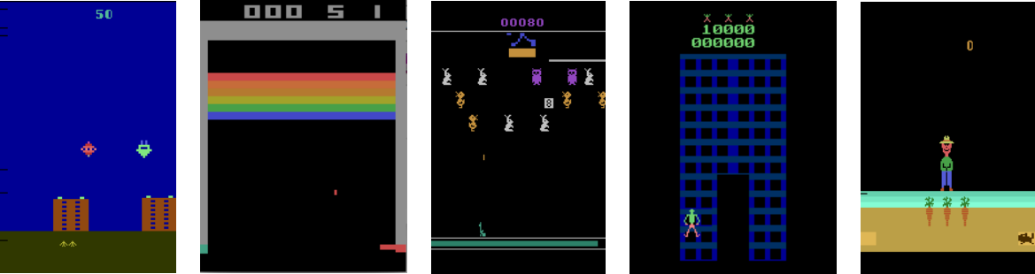
With ACER as baseline, we apply our algorithm to image based Atari games. We only tested on discrete control problems with ACER, and the environments we tested on are: AirRaid, Breakout, Carnival, CrazyClimber and Gopher. The environments are illustrated in Figure 3.
The experiment settings are similar to Wang et al. (2016), The double-output network consists of a convolutional layer with 32 kernels with stride 4, a convolutional layer with 64 kernels with stride 2, a convolutional layer with 64 kernels with stride 1, followed by a fully connected layer with 512 units. The network outputs a softmax policy and state-action value Q for every action.
Because of the limitation of memory, each thread of ACER only have a replay memory of 5000 frames, which is the only different setting from Wang et al. (2016). Entropy regularization with weight 0.001 is also adopted, and the discount factor , importance weight truncation . Trust region updating is used as described in Wang et al. (2016), and all the settings of trust region update remain the same. ACER without trust region update is not tested in this paper.
The results of our pretraining method based on ACER with trust region update is illustrated in Figure 4. All of the environments are image based Atari games. All the lines have the same meaning as Figure 2, and it is obvious that ACER with pretraining process outperforms initial ACER.
Unlike DDPG, the performance of learned policies does not fall after pretraining process ends. This is because for stochastic discrete control, a random policy and a random state-action value estimator always satisfies constraint (1), hence defined in (7) is always zero, and defined in (8) is policy gradient based on expert demonstrations, similar to original from baseline ACER, therefore the performance of learned policies does not fall after pretraining.
Note that learning with expert demonstrations use the same amount of simulation steps as baseline algorithms, our pretraining method is more simulation efficient than baselines.
6 Conclusion
In this work, we propose an extensive method that pretrains actor-critic reinforcement learning methods. Based on Theorem 1, we design a method that takes advantage of expert demonstrations. Our method does not rely on the global optimal assumption of expert demonstrations, which is one of the key differences between our method and IRL algorithms. Our method pretrains policy function and state-action value estimators simultaneously with gradients (9) and (10). With experiments based on DDPG and ACER, we demonstrate that our method outperforms the raw RL algorithms.
One limitation of our framework is that it has to estimate the advantage function for expert demonstrations, and the framework is not suitable for algorithms like A3C Mnih et al. (2016) and TRPO Schulman et al. (2015) that only maintain a value estimator . On the other hand, the fact that expert demonstrations perform better is not considered during pretraining of policies (Equation (8)). We left these extensions in our future work.
Acknowledgments
This work was supported by National Key R&D Program of China (No. 2016YFB0100901), and National Natural Science Foundation of China (No. 61773231).
References
- Abbeel and Ng [2004] Pieter Abbeel and Andrew Y Ng. Apprenticeship learning via inverse reinforcement learning. In Proceedings of the twenty-first international conference on Machine learning. ACM, 2004.
- Bhatnagar et al. [2009] Shalabh Bhatnagar, Richard Sutton, Mohammad Ghavamzadeh, and Mark Lee. Natural actor-critic algorithms. Automatica, 45(11), 2009.
- de la Cruz et al. [2017] Gabriel V. de la Cruz, Jr., Yunshu Du, and Matthew E. Taylor. Pre-training neural networks with human demonstrations for deep reinforcement learning. Technical report, September 2017.
- Degris et al. [2012] Thomas Degris, Martha White, and Richard S Sutton. Off-Policy Actor-Critic.pdf. Icml, 2012.
- Gu et al. [2017] Shixiang Gu, Timothy Lillicrap, Zoubin Ghahramani, Richard E Turner, and Sergey Levine. Q-Prop : Sample-Efficient Policy Gradient with An Off -Policy Critic. ICLR, 2017.
- Heess et al. [2015] Nicolas Heess, Gregory Wayne, David Silver, Tim Lillicrap, Tom Erez, and Yuval Tassa. Learning continuous control policies by stochastic value gradients. In Advances in Neural Information Processing Systems, pages 2944–2952, 2015.
- Hester et al. [2017] Todd Hester, Matej Vecerik, Olivier Pietquin, Marc Lanctot, Tom Schaul, Bilal Piot, Andrew Sendonaris, Gabriel Dulac-Arnold, Ian Osband, John Agapiou, et al. Learning from demonstrations for real world reinforcement learning. arXiv preprint arXiv:1704.03732, 2017.
- Ho and Ermon [2016a] Jonathan Ho and Stefano Ermon. Generative adversarial imitation learning. In Advances in Neural Information Processing Systems, pages 4565–4573, 2016.
- Ho and Ermon [2016b] Jonathan Ho and Stefano Ermon. Generative Adversarial Imitation Learning. In Nips, pages 4565–4573, 2016.
- Ho et al. [2016] Jonathan Ho, Jayesh Gupta, and Stefano Ermon. Model-free imitation learning with policy optimization. In International Conference on Machine Learning, pages 2760–2769, 2016.
- Kakade and Langford [2002] Sham Kakade and John Langford. Approximately Optimal Approximate Reinforcement Learning. Proceedings of the 19th International Conference on Machine Learning, pages 267–274, 2002.
- Kingma and Ba [2014] Diederik Kingma and Jimmy Ba. Adam: A method for stochastic optimization. arXiv preprint arXiv:1412.6980, 2014.
- Lakshminarayanan et al. [2016] Aravind S Lakshminarayanan, Sherjil Ozair, and Yoshua Bengio. Reinforcement Learning with Few Expert Demonstrations. Neural Information Processing Systems - Workshop on Deep Learning for Action and Interaction, 2016.
- Lillicrap et al. [2015] Timothy P Lillicrap, Jonathan J Hunt, Alexander Pritzel, Nicolas Heess, Tom Erez, Yuval Tassa, David Silver, and Daan Wierstra. Continuous control with deep reinforcement learning. arXiv preprint arXiv:1509.02971, 2015.
- Mnih et al. [2015] Volodymyr Mnih, Koray Kavukcuoglu, David Silver, Andrei A Rusu, Joel Veness, Marc G Bellemare, Alex Graves, Martin Riedmiller, Andreas K Fidjeland, Georg Ostrovski, et al. Human-level control through deep reinforcement learning. Nature, 518(7540):529–533, 2015.
- Mnih et al. [2016] Volodymyr Mnih, Adria Puigdomenech Badia, Mehdi Mirza, Alex Graves, Timothy Lillicrap, Tim Harley, David Silver, and Koray Kavukcuoglu. Asynchronous methods for deep reinforcement learning. In International Conference on Machine Learning, pages 1928–1937, 2016.
- Munos et al. [2016] Rémi Munos, Tom Stepleton, Anna Harutyunyan, and Marc G. Bellemare. Safe and Efficient Off-Policy Reinforcement Learning. arXiv, (Nips), 2016.
- Ng and Russell [2000] Andrew Ng and Stuart Russell. Algorithms for inverse reinforcement learning. Proceedings of the Seventeenth International Conference on Machine Learning, 0:663–670, 2000.
- Piot et al. [2014] Bilal Piot, Matthieu Geist, and Olivier Pietquin. Boosted bellman residual minimization handling expert demonstrations. In Joint European Conference on Machine Learning and Knowledge Discovery in Databases, pages 549–564. Springer, 2014.
- Schulman et al. [2015] John Schulman, Sergey Levine, Michael Jordan, and Pieter Abbeel. Trust Region Policy Optimization. Icml-2015, page 16, 2015.
- Silver et al. [2014] David Silver, Guy Lever, Nicolas Heess, Thomas Degris, Daan Wierstra, and Martin Riedmiller. Deterministic policy gradient algorithms. In Proceedings of the 31st International Conference on Machine Learning (ICML-14), pages 387–395, 2014.
- Silver et al. [2016] David Silver, Aja Huang, Chris J Maddison, Arthur Guez, Laurent Sifre, George Van Den Driessche, Julian Schrittwieser, Ioannis Antonoglou, Veda Panneershelvam, Marc Lanctot, et al. Mastering the game of go with deep neural networks and tree search. Nature, 529(7587):484–489, 2016.
- Sutton et al. [1999] Richard S. Sutton, David Mcallester, Satinder Singh, and Yishay Mansour. Policy Gradient Methods for Reinforcement Learning with Function Approximation. Advances in Neural Information Processing Systems 12, pages 1057–1063, 1999.
- Syed and Schapire [2008] Umar Syed and Robert E Schapire. A game-theoretic approach to apprenticeship learning. In Advances in neural information processing systems, pages 1449–1456, 2008.
- Syed et al. [2008] Umar Syed, Michael Bowling, and Robert E Schapire. Apprenticeship learning using linear programming. In Proceedings of the 25th international conference on Machine learning, pages 1032–1039. ACM, 2008.
- Todorov et al. [2012] Emanuel Todorov, Tom Erez, and Yuval Tassa. Mujoco: A physics engine for model-based control. In Intelligent Robots and Systems (IROS), 2012 IEEE/RSJ International Conference on, pages 5026–5033. IEEE, 2012.
- Wang et al. [2016] Ziyu Wang, Victor Bapst, Nicolas Heess, Volodymyr Mnih, Remi Munos, Koray Kavukcuoglu, and Nando de Freitas. Sample efficient actor-critic with experience replay. arXiv preprint arXiv:1611.01224, 2016.