Nonautonomous gradient-like ODEs on the circle:
classification, structural stability and autonomization
Abstract
We study a class of scalar differential equations on the circle . This class is characterized mainly by the property that any solution of such an equation possesses exponential dichotomy both on the semi-axes and . Also we impose some other assumptions on the structure of the foliation into integral curves for such the equation. Differential equations of this class are called gradient-like ones. As a result, we describe the global behavior of the foliation, introduce a complete invariant of uniform equivalency, give standard models for the equations of the distinguished class. The case of almost periodic gradient-like equations is also studied, their classification is presented.
To Jürgen, with thanks and best wishes
Keywords: Nonautonomous ODE, integral curves, foliation, uniform equivalence, classification, structural stability, almost periodic
MSC2010: 34C27, 34C40, 34D30, 70G60
1 Introduction
In 1973 a short note [21] was published where for nonautonomous vector fields (NVFs) given on a smooth closed manifold a definition of uniform equivalency of two such NVFs was given and on this basis the structural stability of nonautonomous vector fields was defined. When a class of structurally stable nonautonomous vector fields was selected, the invariant determining the uniform equivalence was found, Morse type inequalities connecting the topology of and the set of its integral curves were derived. When these results were announced, articles on nonautonomous nonlinear dynamics were rather rare (except, of course, periodic in time systems), though they existed, see, for instance, [26, 37]. Now the interest to the nonautonomous dynamics became much more intensive, several recent books demonstrate this [16, 5, 35]. This gave us a kick to return to this theme.
In this paper we present proofs of some statements of [21] for the one dimensional situation, that is when is the circle . It is worth noting that one dimensional case itself was not discussed in [21] at all.
We study a class of nonautonomous scalar differential equations of the type
where scalar function is 1-periodic in and defines a uniformly continuous map to the space of –smooth 1-periodic functions in , . We consider this space with -norm, thus becomes the Banach space. The space of such maps becomes a Banach space if we endow it with the norm where means the norm in An ordinary differential equation (ODE) determines a foliation of the extended phase space into integral curves (graphs of the solution). Henceforth, we consider the manifold with its uniform structure of the direct product of the standard uniform structure on given by the metrics and metrics on induced from
Two such ODEs are called uniformly equivalent if their related foliations are equimorphic (see below in more details). Below we shall present four assumptions on the class of ODEs under consideration. When they hold we call the equation to be gradient-like one. For equations from this class we prove the following properties:
- •
A gradient-like ODE is structurally stable w.r.t. perturbations within the class of uniformly continuous maps ;
- •
ODEs of this class are rough that is a conjugating equimorphism can be chosen close to the identity map if a perturbation is small enough;
- •
A combinatorial type invariant is introduced which is the complete invariant of the uniform conjugacy for the gradient-like ODEs;
- •
for each gradient-like ODE there is an uniformly equivalent asymptotically autonomous ODE on ;
- •
if a gradient-like ODE is in addition almost periodic in uniformly w.r.t. , then this ODE is uniformly equivalent to an autonomous scalar ODE with simple zeroes.
The results can be also formulated and proved similarly for the case , a segment, as well, in this case it is assumed the boundary curves be integral curves of the differential equation to avoid some complications. The exposition in the paper is carried out for the case .
The beginning of the study of nonautonomous vector fields from the viewpoint of their roughness and their structure was initiated by L. Shilnikov, our joint note [21] was the first result in this direction. The idea itself on the necessity of extending the notion of roughness (structural stability) [1] onto nonautonomous vector fields goes back to A.A. Andronov and was publicized by his wife and collaborator E.A. Leontovich-Andronova in her talk at the III All-Union USSR Mathematical Congress [17].
The first problem here was to find a proper equivalency relation for two nonautonomous vector fields which could be served for a basis of the classification. By that time there existed mainly two approaches to the study of nonautonomous systems. The first one goes back to Bebutov and his translation dynamical system in the space of bounded continuous functions (see [28]). That approach was transformed later into the theory of skew product systems [37]. The second approach was the study of a nonautonomous system itself but the problem of the equivalency of two such systems was not formulated that time.
2 Nonautonomous vector fields
Let be a -smooth closed manifold and be the Banach space of -smooth vector fields on endowed with -norm. A -smooth nonautonomous vector field on (below NVF, for brevity) is an uniformly continuous bounded map . If this map is also -differentiable map, whose derivatives up to order are uniformly continuous, we call to be a -smooth nonautonomous vector field. Every nonautonomous vector field defines its solutions being maps, if and maps, if . As a mapping from , this mapping is of . Solutions of the vector field generate a foliation of the manifold (extended phase space) into its integral curves Henceforth we consider the manifold with its standard uniform structure (see, for instance [15]). All uniformly continuous maps of to itself are considered with respect to this uniform structure. Recall that a homeomorphism of a uniform space is called an equimorphism, if both mappings are uniformly continuous.
An equivalence relation for nonautonomous vector fields proposed in [21] is as follows.
Definition 1
Two NVFs are uniformly equivalent if foliations are uniformly equivalent, that is there is an equimorphism respecting foliations (i.e. sending every integral curve of to an integral curve of preserving its orientation in ).
It is clear that this equivalency relation distinguishes NVFs in which the asymptotic behavior of integral curves are different. This relation allows us to introduce the notion of structurally stable NVFs.
Definition 2
An NVF is called structurally stable, if there is a neighborhood of in the space such that all NVFs in this neighborhood are uniformly equivalent.
The development of the modern theory of (autonomous) dynamical systems showed that the topological equivalency relation is in fact too rigid to get a classification of multidimensional dynamical systems: the structure of such a system can be extremely complicated [9, 10] due, in particular, to the phenomena like Newhouse ones [29, 30, 11].
Nonetheless, this equivalency relation is good enough to classify relatively simple (Morse-Smale) systems, though even in this case the classifying invariant become comparable in its complexity with the structure of a systems itself [13]. This is the achievements of the recent time, at times when this theory started, it was not known.
3 One dimensional gradient-like NVFs
From now on in this paper we consider NVFs on the unique closed smooth 1-dimensional manifold, that is on a circle . We formulate first the restrictions on NVFs which will allow one to classify these vector fields. Let be a (1-periodic) coordinate on , then a NVF defines a scalar ordinary differential equation (ODE, for brevity)
| (1) |
with 1-periodic in function Here is continuous in both variables and uniformly continuous w.r.t. , differentiable in uniformly w.r.t. . Hence, the usual existence and uniqueness theorem is valid for this ODE and any its solution is extended in on the whole . Recall that an integral curve of the equation (below IC, for brevity) is the graph of the related solution in the extended phase space . Thus the extended phase space is foliated into integral curves. We intend to classify these equations w.r.t. the uniform equivalency relation using some combinatorial invariant to be defined later on. To do this, we impose some restrictions on the class of NVFs under consideration.
The first of these restrictions is the following
Assumption 1
Any solution of possesses exponential dichotomy both on and [27].
Definition 3
Let be a solution of the equation . One says that this solution satisfies the exponential dichotomy of the stable type on the semi-axis , if there are positive constants such that the linearized at this solution linear ODE satisfies the inequality
for all
Definition 4
Let be a solution of the equation . One says that this solution satisfies the exponential dichotomy of the unstable type on the semi-axis , if there are positive constants such that the linearized at this solution linear ODE satisfies the inequality
for all
Similar notions of exponential dichotomy of the stable and unstable types are defined for the semi-axis . To be more precise, let us present these definitions as well.
Definition 5
Let be a solution of the equation . One says that this solution satisfies the exponential dichotomy of stable type on the semi-axis , if there are positive constants such that the linearized at this solution equation satisfies the inequality
for all .
Definition 6
Let be a solution of the equation . One says that this solution satisfies the exponential dichotomy of the unstable type on the semi-axis , if there are positive constants such that the linearized equation satisfies the inequality
for all
It follows from the Hadamard-Perron theorem [2] that for a solution to possessing the exponential dichotomy of stable type on there is its uniform neighborhood such that all solutions of the equation (1) starting at within exponentially fast tend to this IC as Moreover, such can be chosen in such a way that a quadratic Lyapunov function would exist in and lateral boundary curves of this are the level lines of the Lyapunov function. Recall how to construct such a function (see, for instance, [8]). Let us write down the equation near the integral curve using local variables . Then the equation transforms into the form
| (2) |
Since the map is bounded and uniformly continuous, the following estimate holds
| (3) |
where continuous function satisfies the conditions as
Let us introduce a function
| (4) |
The improper integral converges uniformly w.r.t. and defines a bounded positive function which is also bounded away from zero. Indeed, one has an estimate
Denote . Then the estimate holds
Thus for function the two-sided estimate is valid
| (5) |
Now let us show be a Lyapunov function for the equation (2) in a neighborhood of its solution . This means that for any initial point the following estimate for the derivative of along a solution through to the equation (2) takes place
Differentiation of gives Hence we get
Therefore one has
Due to the estimate (3), the function within square brackets can be made less than choosing small enough. Let us observe that the derivative of along the system at the point is the inner product of and the tangent vector to the integral curve at the point. From the estimate obtained it follows that at a fixed along the curve the inner product in bounded away from zero uniformly in . Fixing small enough gives an uniform neighborhood of the solution defined as
Now we consider again the equation (1). Henceforth we denote the section in Suppose an integral curve possesses exponential dichotomy of the stable type on . Then all ICs through initial points being close enough to the point at possess also the exponential dichotomy of the same type. This implies a set of traces on the section for all ICs with the exponential dichotomy of stable type on be open and therefore to consist of a collection of disjoint intervals (the cardinality of this collection of intervals is maximum countable). Thus, the set of points on the section through which ICs with exponential dichotomy of the unstable type on pass, form a closed set. The cardinality of this set is an interesting question when the Assumption 1 holds. Our further goal is to distinguish a class of NVFs that are rough and can be classified somehow. This requires of more rigid conditions on the behavior of their ICs. We shall call the set of ICs with exponential dichotomy of the stable type on by a stable bunch if all of them have the same asymptotic behavior, i.e. any two solutions from this stable bunch satisfy inequality , as . In fact the union of all IC of the same stable bunch are a global stable manifold for any IC from this bunch. The boundaries of a stable bunch consists of one or two ICs which possess exponential dichotomy of the unstable type on
Similar properties are valid for ICs which possess the exponential dichotomy on semi-axis Here we define an unstable bunch as the union of all ICs that possess exponential dichotomy of the unstable type on semi-axis Then our next assumption is the following
Assumption 2
. There are finitely many stable bunches and finitely many unstable bunches.
The traces on of those ICs which belong to one stable bunch is an interval. Extreme points of this interval correspond to ICs that possess exponential dichotomy of the unstable type of semi-axis . Similarly, the traces of ICs from one unstable bunch on is an interval and its extreme points correspond to those ICs which possess exponential dichotomy of the stable type on semi-axis . Thus, from this Assumption it follows the existence of finitely many ICs with exponential dichotomy of the unstable type of semi-axis and also does for ICs with exponential dichotomy of the stable type on semi-axis
Our third assumption is
Assumption 3
. No solutions exist such that this solution possesses simultaneously exponential dichotomy of the unstable type on and exponential dichotomy of the stable type on
One more property of the class of ODEs under study has to be discussed. Consider some stable bunch and let be its boundary solutions (left and right, in accordance with the orientation of , respectively). Hence these two solutions possess exponential dichotomy of the unstable type on Choose some solution of the bunch. Due to the Hadamard-Perron theorem (or merely to the existence of a Lyapunov function) one can choose an uniform neighborhood of on within the bunch whose boundary curves are uniformly transversal to solutions of ODE through these boundary curves and these solutions enter to the neighborhood and stay there forever. Similarly, for the solution there is its uniform neighborhood with the property of uniform transversality of its boundary curves but all solutions through this neighborhood leave at some specific for such solution. Without loss of generality we suppose not intersecting and we can choose them as thin as we wish. Now an important question arises: consider for the semi-strip between the right boundary curve of and left boundary curve of . Solutions within this semi-strip enter to it from the left and leave it from the right boundary curve. These solutions cannot stay in this semi-strip for all , since all of them belong to one stable bunch. Is the passing time through this semi-strip is uniformly bounded for all such solutions? The answer to this question is essential for constructing equimorphism which conjugates equivalent ODEs. We shall present below an example of a nonautonomous ODE that shows the answer to this question is generally negative. Therefore this property has to be imposed to avoid a structural instability. To this end, let us choose a sufficiently thin disjoint neighborhoods of all ICs which possess exponential dichotomy of the unstable type on . Also we select by one IC from every stable bunch and choose their thin disjoint neighborhoods . These all neighborhoods can be chosen disjoint.
Assumption 4
For any there are neighborhoods such that the passage time of ICs from one boundary curve to another one is bounded from above.
Now we shall call scalar ODEs on which obey Assumptions 1-4 being gradient-like.
To demonstrate the essentiality of the assumptions imposed, we present examples of differential equations (1) showing that violating any of these three assumptions may give an ODE being nonrough. Our first example was found in [19] and shows that if there is a solution that fails to possess the exponential dichotomy on some of two semi-axes , then the equation may become nonrough and its structure changes at a perturbation. Consider a nonautonomous differential equation on the circle with coordinate
The equation is reversible w.r.t. the involution and the involution Recall, this means that if is a solution to the equation, then so does , that is and .
As this equation tends to the autonomous differential equation given as that has a nonhyperbolic equilibrium The equation considered as nonautonomous has the following foliation onto ICs. There are four stationary solutions Two of them, possess exponential dichotomy on , the first one is asymptotically stable and the second is asymptotically unstable. More two stationary solutions do not possess the exponential dichotomy neither on no on ICs corresponding to stationary solutions divide into four strips. All ICs in each strip go from one stationary solutions (at ) to another one (at ).
Now we take into account in the equation the rapidly decaying term . Solutions stay unchanged and have the same type of dichotomies. Let us consider the invariant strip with its foliation into ICs. Note that One can prove
Lemma 1
There are two special ICs in this strip. One of them is monotonically increasing and tends to as but tends to as . Another one is also monotonically increasing and is defined by reversibility as where is the solution for .
Two special solutions indicated in Lemma do not possess the exponential dichotomy on either (for ) or on (for ). Observe that the straight-line is transversal to ICs intersecting it. All ICs between two special ones intersect this straight-line and tend to as and to as and thus possess the exponential dichotomy. Other ICs lying in the strip below or above do not possess exponential dichotomy on the related semi-axes since they tend in some direction in time to nonhyperbolic solution ( or ). The behavior of ICs in the strip is similar.
This ODE under consideration changes its uniform structure under perturbation. Indeed, consider a perturbed equation with small positive . One can verify that two new bunches have appeared for small , one stable and one unstable. They arise because of the bifurcation, when nonhyperbolic equilibria on bifurcate into two close hyperbolic equilibria. The related foliations are shown in Fig.1. The structure and bifurcation presented is similar to that observed in the Ricatti equation

The second example shows that the violation of the third assumption leads to a structurally unstable ODE. Consider an ODE that has a solution with exponential dichotomy of the unstable type on and let a point be its trace on the section . Suppose the ODE under consideration is such that IC through possesses exponential dichotomy of the stable type on . This implies that there is a sufficiently thin uniform neighborhood of this IC on within which the only IC through lies in entirely for all . If for this ODE two first Assumptions hold, then point serves the boundary point of two intervals corresponding two neighboring stable bunches. Their other boundaries (to the left and to the right from ) on are points (these two points may coincide if the closure of two intervals make up ). Let choose by one IC from both stable bunches. Denote them as The minimal distance between related ICs on is some positive number (Fig.2)
Now we perturb the ODE in such a way that the perturbed ODE would have one IC with the dichotomy of the unstable type on close enough on to former one through and another IC with the dichotomy of the stable type on being close enough on to former IC through . This perturbation can be chosen in two ways as shown in Fig.2. Since the uniform equivalence preserve asymptotic behavior of ICs, these two ODEs are not uniformly equivalent.

a) Degenerate IC

b) Two types of bifurcation
To present an example that demonstrates a possibility to be unbounded for the time of passage from one boundary curve to another one in a transitory strip, we construct an example of equation on the segment instead of . It is easy to glue two such strips to obtain an example on This shows the Assumption 4 be essential.
Consider the semi-bounded strip with coordinates and choose an increasing sequence of numbers such that and as Within segments in given as , we take the function independent on and the same for all such segments. Function is of class , odd and defined as follows
We choose the function independent in (autonomous) for all in semi-strips and . Finally, in rectangles , of the constant length we defined in such a way that is positive for with the related foliation into integral curves within such the rectangle as in Fig.3.
Its specifics is that the solution from the left region goes up and intersects the line between and but solution goes up and cut the line at Similarly, solutions and from the right region, as decreases, intersect the line respectively at and between and . All this guarantees that
- •
each integral curve, except , intersects the line entering thus to the strip where the equation is such solution possesses exponential dichotomy of the stable type on ;
- •
there are countably many solutions of the full equation which coincide with on the segment have their passage time from to greater than and hence these times unbounded.
4 Examples of gradient-like scalar ODEs
Here we present several simple examples of scalar equations of the gradient type on . The first example is trivial, it is an autonomous scalar ODE with a smooth -periodic having only simple zeroes ( at such a zero ) and hence there are only finitely many zeroes (equilibria). Due to compactness of all solutions to ODE tend, as , to some of its equilibrium, their simplicity guarantees the exponential dichotomy of the related constant solutions on , as well as the exponential dichotomy on the semi-axis or for all solutions that tend to this constant solution as or , respectively.
The second example is less trivial but also well known. Consider a nonautonomous doubly periodic equation . The function is -periodic in both variables and smooth (in fact, it is sufficient to be continuous in and differentiable in with a continuous derivative in ). Then the Poincaré map in is well defined. This map is a diffeomorphism (at least ) and has a Poincaré rotation number. Suppose this number is rational with incommensurate . Then by the Poincaré theorem (see, for instance, [14]) this map has a periodic orbit of the period and any other orbit is either periodic one with the same period or tend to a periodic orbit as ( is the number of iterations) and to a periodic orbit (possibly to another one) as . Suppose all these periodic orbits are hyperbolic, i.e. at any periodic orbit. Then there are only finitely many periodic orbits and hence this nonautonomous ODE is of the gradient type.
The third example is a so-called asymptotically autonomous scalar ODE [26, 39, 36]. Suppose a differential equation on be given such that as and as where the limit is taken in the space We assume that both ODEs on the circle with functions have only simple zeroes as in the first example. Then any IC of the given equation asymptotically approaches as to some , , and asymptotically approaches as to some , [26]. It follows from here that any integral curve possesses an exponential dichotomy both on In order the equation would be gradient-like, one needs to require in addition that no IC exists that asymptotically tends as to a stable zero of and as does to an unstable zero of . Then this ODE is a nonautonomous gradient-like one. As an example of such the equation one can construct a glued differential equation. We take a rough scalar autonomous equation with the function and another rough scalar autonomous equation with the function . The nonautonomous equation is glued as follows. Let for the equation with is considered, and for does the equation with In the layer between two sections we can specify a smooth foliation in such a way that traces of ICs for the equation with would join with traces of ICs to the equation with and all curves of the foliation in this layer would intersect transversely sections , . This makes the complete foliation smooth. The derivatives in for ICs will give gradient-like nonautomous ODE.
In the similar way examples of a nonautonomous asymptotically periodic scalar gradient-like ODEs can be constructed. To that end, one needs to choose two periodic limiting ODEs as in the example 2 above (they play the role of limiting equations at ) given by functions and being periodic in with possibly different periods. Suppose their related foliations into ICs are disposed lower of (for ) and above of (for ). Then we get on two 1-periodic in functions and being two points in the Banach space Let us join these points by a smooth compact path with the parametrization . Then we get a glued function which defines the nonautonomous ODE on and coincides with when and does with when The only thing we need to care about is that in a middle part of traces of stable periodic solutions to negative limiting ODE (for ) would not be connected with periodic solutions of positive limiting ODE being unstable hyperbolic for . This is achieved by a small perturbation of the ODE in the layer.
5 The properties of gradient-like NVFs on and u-invariant
In this section we define an invariant which is able to recognize different gradient-like ODEs. This invariant is of combinatorial type, i.e. it is defined by the finite set of ingredients.
To construct the invariant we begin with some assertions necessary for the construction.
Lemma 2
For a gradient-like scalar ODE at least one solution with exponential dichotomy of the unstable type on always exists, as well as at least one solution with exponential dichotomy of the stable type on .
Proof. Suppose, to the contrary, a gradient-like ODE has not any solution with exponential dichotomy of the unstable type on This implies that there exists the unique stable bunch and the union of traces on of ICs from this bunch is the whole Choose some IC from this bunch. There is an uniform neighborhood of such that all ICs starting within stay inside it for all Thus, one can choose such a neighborhood for any IC of the bunch. The union of these neighborhoods covers , thus the intersection of these neighborhoods with the section gives a cover of Compactness of allows one to select a finite cover and consequently a finite set of ICs around which these neighborhoods have been chosen. Denote related traces on of these ICs as points enumerated in accordance with the orientation of . Take some positive number For any there is such that for the distance between traces of those ICs, which start at at extreme points of , on the section will be lesser than Thus for the distances between traces of any two ICs from the bunch will be lesser than On the other hand, they should cover This contradiction proves the lemma. The similar proof holds true for the dichotomy of the stable type on
Now we shall define a combinatorial invariant which distinguishes two uniformly nonequivalent gradient-like ODEs on . Let a gradient-like ODE be given. Take the section . We assume that is oriented by the coordinate. On the section we consider the traces of all ICs which have the dichotomy of unstable type on Denote this set of points as where the order from to is defined by the orientation of Similarly, we consider the traces of all ICs which have the dichotomy of stable type on Denote them as where the order from to is also defined by the orientation of These two sets of points on do not intersect in accordance with the Assumptions 1-3. Due to Lemma 2, integers are both positive. We shall call the set of points the equipped set of points.
Definition 7
Two equipped sets on will be called equivalent, if there is a homeomorphism such that sends the set of the first equipped set onto the set of the second equipped set, and the set of the first equipped set to of the second equipped set.
A class of equivalent equipped sets will be called u-invariant. The main result of the paper is the following theorem
Theorem 1
Two nonautonomous scalar gradient-like ODEs on are uniformly equivalent, iff they have the same u-invariant.
It is clear that two uniformly equivalent ODEs on have the same u-invariant. The proof of the inverse assertion is the main task.
Gradient-like ODEs possess also the property of structural stability. This notion was introduced by Andronov and Pontryagin in 1937 [1] for autonomous vector fields on 2-dimensional sphere (or on a disk with the proper assumptions on the orbit behavior on the boundary cicrle) and was studied in many details, first on sphere (Leontovich-Andronova, Maier [18]) and then on the torus (Maier). The final result for any smooth closed 2-dimensional manifold was done by Peixoto [31]. Multidimensional case was studied first by Smale [32] who defined the class of vector fields and diffeomorphism which were called later Morse-Smale systems. Their study lasts till now [12, 13].
Leaning on Theorem 1 we will also prove
Theorem 2
A gradient-like NVF on is rough, that is, for any there exists such that all NVFs in the -neighborhood of in the space are uniformly equivalent to and an equimorphism realizing this equivalence can be chosen -close to the identity mapping . Moreover, all shifted NVFs are also rough with the same
Proofs of both theorems will be outlined in the next two sections.
6 A method to construct an equimorphism
To demonstrate the method of constructing an equimorphism for two gradient-like ODEs with the same u-invariant, we present here first the simplest possible situation when both differential equations are linear. It gives, in a sense, the simplest uniform version of the Grobman-Hartman theorem [14]. For the case of two gradient-like nonlinear ODEs the local construction is similar.
Consider two scalar linear homogeneous differential equations
| (6) |
Denote the solution of (6) with the condition and let be the similar solution for the second equation
We assume both these linear ODEs to possess exponential dichotomy of the stable type on
| (7) |
and the same holds for the second equation with constants
We defined above a Lyapunov function (4) for such equation. For equations under consideration we denote related functions as
From expressions for the inequalities follow
| (8) |
| (9) |
where
Observe that functions obey the equations
Our goal in this section is to prove that the map from the semi-strip in the plane around onto the semi-strip in the plane around is an equimorphism. The strip is defined by its boundary curves and , , where is some positive constant. This semi-strip contains the right curve but does not contain the left one . Similar formulae define the strip with the change .
Let us define the map . First we change the coordinates in both semi-strips. Instead of we take as new coordinates , similarly, we change to In accordance with the formulae for Lyapunov functions, these coordinate transformations are smooth in both variables and linear in (respectively, ) with uniformly bounded coefficients being uniformly bounded away from zero. Then the map is given as follows. Take any point and consider the integral curve of the first equation through this point. This curve intersects transversely the level line of the Lyapunov function defined by at some time . We fix some smooth monotone function given as with positive uniformly bounded from above and from zero: For instance, as a such map one can take the identical map To facilitate the exposition, we take just this identical map. Then the point on the right boundary of with coordinates is transformed at the point on the right boundary curve of On the integral curve of the second equation through this latter point we choose that its point whose -coordinate is . Then -coordinate of this point is
Integral curve through the point is
This curve intersects the boundary level line at the point with coordinates where is found from the equation
| (10) |
Denote the left hand side of this equation. Function is a solution to the equation existing by the implicit function theorem.
Integral curve of the second equation through the point is given as (its second coordinate)
For the point the time variable on this curve is -coordinate of this point is found from the equation
| (11) |
The right hand side of the equation (11) will be denoted as Thus the map is given in coordinates as follows
| (12) |
We need to prove the uniform continuity of this map along with its inverse one.
In fact, we need only to prove the uniform continuity of in the strip The uniform continuity of the inverse map is proved in the same way, since the inverse map is defined in the similar way. The uniform continuity of , when it has been proved, allows to extend the map uniquely to the closed strip by the relation
The uniform continuity of is proved in two steps because the derivatives of is not bounded if we consider the full strip . Therefore we fix some and prove that -pre-image in of the line is a curve being the graph of a function and this function obeys estimates Moreover, if then both tend also to zero. Thus choosing small enough we get that the semi-strip is transformed on the semi-strip in which belongs to the semi-strip Since -coordinate preserves by this gives uniform continuity near the line . In the closed semi-strip the derivatives of are uniformly bounded and this guarantees the uniform continuity for there.
Now consider in pre-images of the Lyapunov function level lines defines by constants in . First we will show that this curve is given as for which the inequalities hold
and tend to zero, if .
To this end, we solve the equations (12) w.r.t. setting . Since the value of preserves, then the solutions will give a function and we need only to estimate them. These functions are given in the following way
Here function is a solution of the equations (11) with . From this equation an estimate for the difference is derived using the exponential dichotomy
We consider small enough positive, so r.h.s. will tend to infinity as but it is finite, if holds fixed. We have a similar estimate from below
Using these estimates for we come to the following estimates for function
| (13) |
These estimates say that the pre-image of any strip in is a strip in lying in the the strip . This implies that for proving uniform continuity one may use estimates for the derivatives of . These derivatives are as follows
and using (11) we get
| (14) |
Therefore, the estimate for in the strip is given as
| (15) |
Now the calculation of derivative
gives the formulae
Thus, we come to the estimate
| (16) |
These estimates for derivatives show the uniform finiteness of derivatives.
Now we are able to complete the proof of the uniform continuity of Choose the metrics in both strips:
Let a positive be given. Put in (13) and take . Take two arbitrary points in at the distance Three cases are possible: i) both belong to the sub-strip ii) both points belong to the sub-strip iii) one point, say , belongs to first sub-strip but belongs to the second sub-strip. In the first case both points belong to the strip . Since and preserves -coordinate, then The same estimate holds for the third case due to estimates for derivatives of . The second case is reduced to the combination of the first and third ones if we joint points by the segment on the right boundary of the semi-strip
The construction gives an equimorphism only in semi-strips and In order to get an equimorphism of the whole strip around and respectively, one needs to conform them along the straight-lines and respectively. In the construction presented it is done automatically since the section is transform to the section For the general case one needs to care about it.
7 Uniform equivalence and structural stability
To prove Theorem 1, we need to construct an equimorphism which transforms the foliation into ICs of the first gradient-like ODE to that of the second ODE. The idea of the construction is close to that performed in the linear case (see above) but with some modifications exploiting the structure of ODEs. The main idea is to construct first an equimorphism in some neighborhood of those ICs whose traces on enter to the equipped set (we call the set of these ICs a skeleton of the ODE) and after that to extend this equimorphism to the whole manifold When an ODE under consideration is gradient-like one, then its skeleton depends continuously on a perturbations in the class of uniformly continuous bounded maps This allows to prove that a conjugating equimorphism can be found to be close to the identity map In the general case of two gradient-like ODEs with the same u-invariant the construction of a conjugating equimorphism is geometrical and requires a detailed description. We present here only some details of this construction. A complete exposition will be done elsewhere.
We start with constructing a sufficiently thin neighborhood of the skeleton of the ODE. As a skeleton we take the following collection of ICs. Consider the equipped set of the ODE. Its -points on are distributed on intervals in formed by the traces of -points (Assumption 3). ICs through -points which belong to the same interval are in the same unstable bunch. Choose IC through the point . This IC belongs to some unstable bunch. The intersection of this bunch with defines some interval whose boundary points are . This implies to possess exponential dichotomy of the unstable type on (we call such IC to be globally unstable). Recall that a sufficiently thin neighborhood of such IC does not contain wholly any IC other than and boundary curves of this neighborhood are uniformly transversal to all ICs passing though points of these curves. Here there is an alternative: either no other points from exist which belong to the same interval or there are several such ICs. In the first case the second ODE also has a corresponding IC which passes through the point of its equipped set and its uniform isolating neighborhood . We can construct equimorphism from to by the method similar to in the preceding section.
In the second case all related ICs belong, as was said, to the same unstable bunch and they are asymptotic to each other as Thus we have to construct a neighborhood for all this collection of ICs from the bunch. All these ICs are globally unstable ones. We choose some isolating uniform neighborhood of IC through point and consider IC through the point There is its isolating neighborhood in fact, many of them being as thin as we need. IC intersects one boundary curve of transversely at some point at . Thus we can choose thin enough in order both boundary curves of would intersect the same boundary curve of transversely and therefore will belong to below some (see Fig.4). Now we proceed in the same way in order to construct a tree-shape neighborhood for all collection from one unstable bunch through (see Fig.4).
The boundaries of the neighborhood are uniformly transverse to ICs but may contain a finitely many angular points where two boundary curves from different adjoin. At such a point the IC through it is transverse to both local smooth boundary curves. This IC possesses exponential dichotomy of the stable type on . We shall distinguish different boundary curve of a tree-shape neighborhood . First, there are two infinite in both directions of time left and right boundary curves. We call them to be outer ones. To specify all boundary curves we call the initial neighborhood for to be a trunk and other attached to the trunk as branches. Then is the left boundary of the trunk drawing from till its intersection with the left boundary curve of the leftmost branch (or till , if the trunk does not have branches to the left). Analogously, we get the right boundary curve made up of the left boundary curve of the trunk till its intersection with the right boundary curve of the rightmost branch. Other boundary curves are of the -shape or of the semi-strip shape and formed by other boundary curves of inner branches, they are semi-infinite and are extended till .

Now we proceed in the similar way constructing neighborhoods involving points related with another unstable bunch, and so forth, till we exhaust all collection of -points in the equipped set. It is clear that the neighborhoods can be constructed not intersecting and situated at a finite distance from each other.
Let us note that this construction does not involve so far -points . Now we continue the construction proceeding in a similar way but starting with ICs through points on and using stable bunches with traces . Thus, we construct the neighborhoods . These neighborhoods are also chosen sufficiently thin in order to be separated from each other and from neighborhoods The -neighborhoods constructed have the following characterization. They contain wholly only those ICs which make up the skeleton. All other ICs either leave the related neighborhood (for instance, for ) when increasing at some finite time. After that such an IC either in finite time enters to some through its lateral boundary curve (leftmost or rightmost one) and this time is uniformly bounded from above for all such ICs (Assumption 4) or such an IC belongs to some stable bunch. In the second case we choose in addition an IC in this stable bunch through angular point on the boundary of and select some its thin uniform neighborhood whose boundary curves are transverse to the boundary curves of (see Fig.5)

For a neighborhood we have a similar assertions with reversing time. In particular, here one needs to choose in addition the neighborhoods of ICs in unstable bunches which we denote as . The passage time from the boundaries of all neighborhoods constructed are uniformly bounded due to Assumption 4.
7.1 Conjugating equimorphism
The construction of an equimorphism transforming one foliation into ICs to another one is performed in two steps. At the first step we define this equimorphism inside of the constructed neighborhoods , . At the second step we extend the equimorphism outside of the union of these neighborhoods defining it wholly on . Since the construction is geometrical, it requires more room than we have here. So, we present only some details, the complete exposition will be done in the paper under preparation.
The basic construction of an equimorphism is performed in a thin semi-strip or around fixed IC of the skeleton. Here is chosen large enough in order all such semi-strips do not intersect each other. It can be also a thin neighborhood of an IC from a stable (then ) or an unstable bunch (then ). A construction of an equimorphism within this semi-strip is the same as in the previous Section 6. It is determined, if one sets an equimorphism on the lateral boundary curve and a homeomorphism on the segment of the bottom (or top) of the semi-strip. Here the levels of the related Lyapunov function plays the main role. The lateral boundary curves of the semi-strips themselves are the level lines of such a function. It requires a neighborhood to be thin enough. We assume below that this construction is given.
It is clear that impossible to set equimorphisms on boundary curves independently for different semi-strips. There are ICs which intersect boundary curves of two different semi-strips and this should be taken into account when constructing. To verify easily that an equimorphism within a semi-strip is extended till the basic IC of this semi-strip we shall set them identically in time for The construction the Section 6 guarantees that equimorphism within the semi-strip transforms the segment to the segment . In the cylinder this by means some homeomorphism respecting the foliation.
In order to demonstrate the main points of the construction and how to conform them to guarantee that any IC of the first ODE would transform by the equimorphism to some IC of the second ODE we discuss two point.
The first point is constructing an equimorphism within a fixed neighborhood To simplify notations, we omit the index . We start with the leftmost boundary curve of the neighborhood. To the right from this curve the first IC from the skeleton is situated. We denote it (changing the numeration if necessary). We first construct the equimorphism in the strip between these two curves and Observe that on the only angular point can exists (no angular points is also possible, if no branches attach to the trunk from the left side). If there is an angular point, we cut the strip into two semi-strips by a segment through the angular point. For the second ODE there is the similar strip which is divided by the angular point on the section For each semi-strip and we construct the Lyapunov function with its levels. This is possible if the neighborhood is chosen thin enough. After that we define some equimorphism on the boundary curve and extend it to the strip as equimorphism by the same construction as in the previous section. This equimorphism is extended till the closure of the strip, hence it is defined on .
To the left from there is the only , its rightmost boundary curve has a nearest IC being globally stable on Any IC passing through at some intersects at an only point at some and the difference is uniformly bounded for all such ICs due to Assumption 4. This defines the correspondence between and and hence defines an uniformly continuous map to the related curve of the second ODE. After that we construct the extension of the equimorphism into the strip between and in the same way as above.
For the upper semi-strip we do as in the preceding section: we choose some uniformly continuous map on for defining the map to the analogous left boundary curve for the second ODE for . Then for any point inside we take the IC through . This IC intersect at some point . Let be the related time coordinate. The map transform to the point on through which an IC of the second ODE passes. We choose on this IC a point with the time coordinate
The second point is the extension of the equimorphism from two neighboring semi-strips corresponding to two neighboring -points of the equipped set into a region between them being either of -shape or of a semi-strip. Let and be the related basic ICs for these -points. All IC between them belong to the same -interval, that is ICs leaving left semi-strip through its right boundary curve and ICs leaving right semi-strip through its left boundary curve are asymptotic to each other as Fix some IC from this stable bunch (usually we take as such IC that which go through an angular point where two boundary curves of neighboring semi-strips intersect). For we choose some thin uniform neighborhood of IC such that this neighborhood does not intersect both neighborhoods of and . The equimorphism constructed defines the map on the boundary curves and by ICs it is extended to the boundary curves of the stable IC and after that does to its inner part.
8 Autonomization
In this section we introduce another invariant of uniform equivalency which shows that a gradient-like ODE on is uniformly equivalent to an asymptotically autonomous ODE. Let a gradient-like ODE be given. Then a definite u-invariant corresponds to this ODE. Consider the circle and related points . The numeration in each group (‘‘u’’ and ‘‘s’’) is done in accordance with the orientation of . The section is divided into intervals with points . Each interval contains some number -points arranged in the orientation order, Observe that some may be zeroes.
Next we choose a smooth function on whose all zeroes are simple. In particular, zeroes at the points are all with positive derivatives and no other zeroes of this type exist. Hence, more simple zeroes , with negative derivatives should exist at some points of each interval . The collection of points makes up a complete set of zeroes for
Similarly, there is a smooth function with only simple zeroes, and its zeroes with negative derivatives are just points Then there are exactly simple zeroes with positive derivatives at some points on every interval Again, we assume these be all zeroes of Functions define autonomous ODEs at The scheme of the asymptotically autonomous ODE under construction is the following. Take an annulus (cylinder) on the plane with polar coordinates We mark at the outer boundary zeroes of the function in accordance with the agreement that corresponds to the coordinate on . Similarly, we mark zeroes of at the inner boundary with the same agreement. Now we join points on by the disjoint paths with points on the boundary in accordance with the equipped set. Namely, take the point of the equipped set. There is the unique IC with unstable type exponential dichotomy on This IC belongs to a unique bunch of ICs which possess the unstable type of dichotomy on . This bunch defines two boundary ICs of ODE with the stable type of dichotomy on , that is, two neighboring points of the equipped set. On the interval in the circle between its related zeroes with negative derivatives there is only one zero with the positive derivative. We joint point on with on by a path. In order to avoid intersections of the paths let us cut the annulus along the path constructed. We get a curvilinear rectangle with two boundary curves, (top) and (bottom), and two side boundaries corresponding to the path. We assume that the orientation of top and bottom boundaries corresponds to increasing . Then is at the left upper vertex of the rectangle and is at the left lower vertex.
Take now . If in the equipped set for ODE no -points between and then both belong to the same interval of defined by the -points. This means, due to the construction, that both ICs corresponding to belong to the same unstable bunch. This means that as both these ICs are asymptotically approach to each other. Then we need to join with a path point on with the same point , this path should not intersect the side boundaries, of course. This second path distinguishes a curvilinear triangle in the rectangle and if we cut the rectangle along this second path then we again obtain a rectangle but with the left upper vertex Suppose now that between and in the equipped set there is at least one -point, say (re-enumerating the set of -points one can always regard this). On the interval in defined by two neighboring points we get the ordered set of -points The next -point lies to the right from Now we choose the interval on the bottom boundary between two zeroes with negative derivatives of the function corresponding . Due to the choice of , between these two zeroes there is a unique zero with the positive derivative . Joining by a path points on with the point on gives a sub-rectangle in the rectangle with the side boundaries: the first path (left) and new path (right). Cutting off the sub-rectangle we come to the new rectangle with the left upper vertex instead of and being the left lower vertex. To finish the first step of the induction we connect within the sub-rectangle obtained points by paths with the unique point on corresponding to a zero of with the negative derivative on the interval .
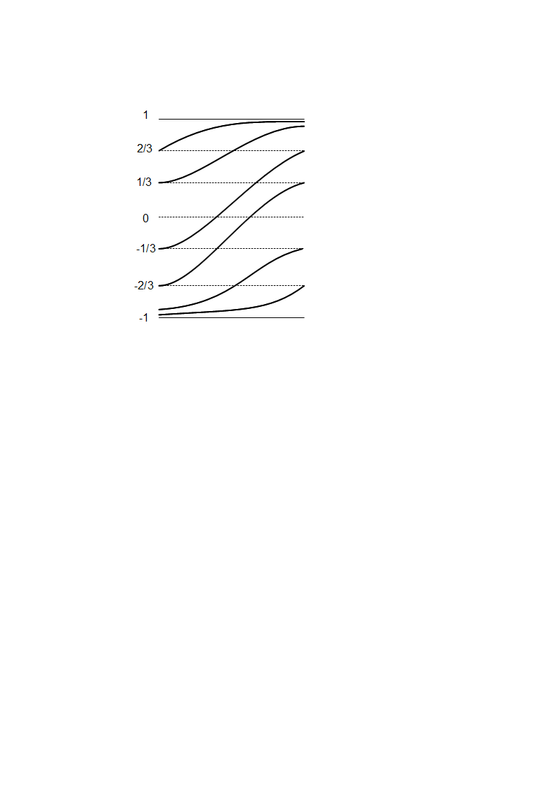
Thus we have made one step of the induction. Repeating this procedure gives the annulus with all paths (see Fig.6). This construction gives the asymptotically autonomous gradient-like ODE with its limiting ODEs defined by functions The following theorem states this.
Theorem 3
For any gradient-like nonautonomous ODE on there is an asymptotically autonomous gradient-like ODE being uniformly equivalent to
Proof. To construct such an ODE we take on the cylinder the foliations generated by for and the foliation for when In the annulus and we construct smooth foliation as in the example above in accordance with behavior of paths constructed. This gives the needed asymptotically autonomous ODE.

9 Almost periodic gradient-like equations on
In this section we apply the theory developed in previous sections to the classical nonautonomous case – almost periodic in time scalar differential equations on the circle
| (17) |
We assume, as above, the equation be gradient-like one. The equation (17) is generated by the map , being almost periodic and therefore uniformly continuous.
Let us recall some notions from the theory of almost periodic functions [24, 7, 25]. A continuous map into Banach space is called almost periodic, if for any there exists a relatively dense set of -almost periods such that for any the following inequality holds
Recall that a subset is relatively dense, if there is a positive number such that any interval contains at least one number
There is another definition of an almost periodic function introduced by Bochner. It relies on the following theorem by Bochner [3]. For a bounded continuous function consider the sequence of shifted functions .
Definition 8
Function is called normal, if for any sequence of its shifts there is a subsequence such that this subsequence converges in the topology of uniform convergence on
Theorem 4 (Bochner)
A continuous function is almost periodic iff it is normal.
Trivial examples of gradient-like almost periodic equation on are the following ones. The first is autonomous differential equation on , , when a -smooth 1-periodic function has only simple zeroes (where ). The second is when is -periodic in and the related Poincaré map on in the period is a diffeomorphism of with a rational rotation number. Then, as is known, all solutions are either -periodic or tend to -periodic solutions as The integer is the same for all periodic solutions. If all periodic solutions have multipliers distinct of unity (i.e. the related periodic points of the Poincaré map are hyperbolic), then this periodic ODE is gradient-like one. A somewhat less trivial example is a small smooth almost periodic perturbation of any of these two examples.
The second example shows that an almost periodic solution can go around infinitely many times when increases (decreases). For instance, any function of the form with any and arbitrary almost periodic function is almost periodic on . In fact, in this case we have a particular example of an almost periodic mapping which takes its values in some metric space with the metrics . Recall that a continuous mapping is almost periodic, if for any there is a relatively dense set such that for any the following inequality holds
For our case with the standard metrics ,
Another equivalent definition of a.p. mapping is due to Bochner: any sequence of shifts is precompact in the topology of the uniform convergence of mappings
For the case of a function be an almost periodic function with values on if it is almost periodic as a function understanding as being embedded into as
In this section we prove the following theorem
Theorem 5
Suppose a differential equation on is gradient-like and almost periodic in . Then each its solution being unstable on is almost periodic and possesses exponential dichotomy of the unstable type on , and each its solution being stable on is almost periodic one and possesses exponential dichotomy of the stable type on . These a.p. solutions can be united into finitely many pairs – one stable and one unstable – serving the boundary solutions of a closed strip. The union of these strips is . Within such a strip solutions distinct of boundary ones tend to the boundary stable almost periodic solution as and to the boundary unstable a.p. solution as . This ODE is uniformly equivalent to the autonomous scalar differential equation with a smooth function having simple zeroes on .
To begin with we formulate several auxiliary statements.
Lemma 3
Suppose be an integral curve possessing exponential dichotomy of the unstable type on . Then there is an uniform neighborhood of in such that any IC intersecting this neighborhood belongs to the neighborhood only during a finite time on . The boundary curves of this neighborhood are uniformly transversal to ICs intersecting them.
Such a neighborhood will be called an isolating neighborhood of such integral curve. As such a neighborhood of the IC related to the neighborhood defined by a level of the Lyapunov function corresponding to the solution , corresponding to , can be chosen (see above).
Lemma 4
Suppose some IC of the unstable type on for ODE (17) is given. There is such that if then the boundary curves of an isolating neighborhood for this IC remain uniformly transversal for IC of the equation and this neighborhood contains the only IC which stay wholly in for all
Lemma 5
IC depends continuously on at the ‘‘point’’ .
Proofs of these lemmata can be obtained from standard results of the theory of exponential dichotomy, see [8].
Consider some solution of the differential equation (17) which possesses exponential dichotomy of the unstable type on . Since this equation is gradient-like one, such solution exists and, in virtue of Assumption 3, it also possesses exponential dichotomy of the unstable type on This implies this solution to possess the exponential dichotomy of unstable type on the whole Choose some its isolating neighborhood on and consider any sequence as We need to prove that the sequence of shifted functions is precompact, i.e. a subsequence exists such that the subsequence converges in the topology of uniform convergence on
Since ODE (17) is almost periodic, there exists some subsequence as such that the sequence of shifts converges in the topology of uniform convergence on in the space of continuous maps . Thus, for any there is a such that for any the inequality holds: where the norm is taken in the space The differential equation evidently has the solution If is an isolating neighborhood for IC corresponding to , then its shift on gives the isolating neighborhood of shifted solution. For small enough ODEs with r.h.s. and are close enough and since is rough, then all shifted equations are also rough with the same radius of roughness. In particular, for small enough an equimorphism realizing the uniform equivalence of the foliation onto ICs for ODE with the foliation for ODE is close to the identity map . This implies that in the isolating neighborhood of the solution can lie wholly only one solution of ODE with r.h.s. and this solution has the exponential dichotomy of unstable type on . Thus, we get a unique solution of the ODE with exponential dichotomy of unstable type on Shifting it back in time allows us to get a solution of the same type for the initial ODE (17). We can do the same procedure for changing the sequence and sub-sequences . In such a way, we shall find several solutions with the same type of dichotomy of the initial ODE which are connected by the limiting procedure with . Since there are finitely many solutions with the dichotomy of unstable type on , we break all such solutions into several groups. It is clear that if, using this procedure, we get a solution from the solution and next do it from to , then combining a proper sequence of shifts we get from as well. Thus, solutions from different groups cannot be obtained from each other by the limit. But all solutions from the same group can be obtained from each other by the given procedure. In particular, this means that starting from solution we can get itself using some sequences of shifts. In a sense, one group of solutions corresponds to one periodic orbit and its shifts on the periods for the periodic ODE. Observe, that solutions from one group are separated from each other: these solutions are separated by their uniform isolating neighborhoods.
Thus we proved that shifts of a given solutions with the exponential dichotomy of unstable type on is precompact: its limit sets consists of solutions of one group. Therefore, this solution is almost periodic.
The same considerations work if we start from a solution of ODE (17) with the exponential dichotomy of stable type on . Then we conclude, due to gradient-likeness of (17), that this solution possesses by the exponential dichotomy of stable type on . After that we again break solutions of such type into groups, and so forth. Solutions from different groups of stability cannot coinside and therefore all extended phase manifold is divided into several strips whose boundary ICs are one stable and one unstable ones.
As an immediate application of this theorem, let us consider an almost periodic perturbation of a periodic ODE on . Concerning the unperturbed ODE we assume that its Poincaré map in the period is rough, that is it has a rational rotation number and all its periodic points are hyperbolic. Then this periodic equation is gradient-like and rough. Under a sufficiently small a.p. perturbation near each hyperbolic periodic IC in a unique a.p. IC arises. The type of exponential dichotomy for the a.p. solutions on will be the same as was for the related periodic solution of unperturbed equation. All other solutions will tend to a.p. solutions as Thus we get
Corollary 1
A sufficiently small a.p. perturbation of a periodic ODE with a rough Poincaré map in the period is uniformly equivalent to the autonomous ODE with the same number of its simple zeroes as for the number of periodic orbits for the Poincaré map.
It is worth remarking that if an almost periodic ODE fails to be rough then it may not have any almost periodic solutions at all. For instance, a periodic ODE on having an irrational rotation number and realizing the Denjoy case (for -smooth ) has not any almost periodic solutions. The first such example for an almost periodic case was constructed in [34] (see its more detailed consideration in [23]).
10 Acknowledgement
L.M.L. thanks for a support the Russian Science Foundation (grant 14-41-00044), as well as the Russian Foundation of Basic Research (grants 16-51-10005-КО and 16-01-00324). A part of this research was supported by the Ministry of Education and Science of Russian Federation (project 1.3287.2017, target part).
References
- [1] A. Andronov and L. Pontryagin, Systémes grossiers, Dokl. Akad. Nauk. SSSR v.14 (1937), 247-251.
- [2] D.V. Anosov, Geodesic flows on manifolds of the negative curvature, Trudy Mat. Inst. Steklov., v.90 (1967), 211 pp.
- [3] S. Bochner, Sur les fonctions presque périodiques de Bohr, Comptes rendus, v.180 (1925), 1156-1158.
- [4] I.U. Bronstein, Extensions of Minimal Transformation Groups, Springer Netherlands, 1979.
- [5] D. Cheban, Global Attractors of Non-autonomous Dissipative Dynamical Systems, World Scientific Publishing Co. Pte. Ltd, Singapoure, 2004.
- [6] W.A. Coppel, Stability and asymptotic behavior of differential equations, Heath, Boston, Mass., 1965.
- [7] C. Corduneanu. Almost Periodic Oscillations and Waves, Springer Science+Business Media, LLC, 2009.
- [8] B.P. Demidovich. Lectures on Mathematical Theory of Stability, (in Russian), Nauka, Moscow, 1967.
- [9] S.V. Gonchenko, L.P. Shil’nikov, D.V. Turaev, "On models with non-rough Poincare homoclinic curves", Physica D, 1993, v.62, Nos.1-4, 1-14.
- [10] S.V. Gonchenko, D.V. Turaev, L.P. Shilnikov, Homoclinic tangencies of an arbitrary order in Newhouse domains, in Itogi Nauki Tekh., Ser. Sovrem. Mat. Prilozh. 67, 69-128 (1999) [English translation in J. Math. Sci. 105, 1738-1778 (2001)].
- [11] S.V. Gonchenko, L.P. Shilnikov, D.V. Turaev. On the existence of Newhouse regions near systems with non-rough Poincare homoclinic curve (multidimensional case). Russian Acad. Sci.: Dokl. Math. 47 (1993), no.2, 268-283.
- [12] V.Z. Grines, E. Gurevich, O. Pochinka, Topological classification of Morse-Smale diffeomorphisms without heteroclinic intersection, J. Math. Sci., v.208 (2015), No.1, 81-90.
- [13] V.Z. Grines, T.V. Medvedev, O.V. Pochinka. Dynamical Systems on 2- and 3-Manifolds, ‘‘Developments in Mathematics’’, v.46, Springer International Publishing, 2016.
- [14] P. Hartman. Ordinary Differential Equations, John Wiley & Sons, New York-Toronto-Sydney, 1964.
- [15] J.L. Kelley, General topology, D. Van Nostrand Co., Inc., Princeton, N.J., 1957.
- [16] Kloeden P.E., Rasmussen M. Nonautonomous dynamical systems, Math. surveys and monographs, v.176, AMS, Providence, R.I., 2011.
- [17] E.A. Leontovich-Andronova. On mathematical achievements of the Gorky school by A.A. Andronov, in "Proc. of the III All-Union Mathematical Congress", v.3, USSR Acad. of Sci. P.H., M.: 1958.
- [18] E.A. Leontovich-Andronova, A.G. Maier, On a scheme determining topological structure of the orbit foliation, Doklady AN SSSR, v.103 (1955), N 4.
- [19] L.M. Lerman. On nonautonomous dynamical systems of the Morse-Smale type, PhD thesis, Gorky State Univ., Gorky, 1975, 150 pp.
- [20] L.M.Lerman. On nonautonomous dynamical systems of the Morse-Smale type, Uspekhi Mat. Nauk, v.XXX (1975), No.5, p.195 (Sessions of the Moscow Math. Soc.) (in Russian).
- [21] L.M. Lerman, L.P. Shilnikov. On the classification of structurally stable nonautonomous systems of the second order with a finite number of cells, Soviet Math. Dokl., v.14 (1973), No.2, 444-448 (transl. from Russian: Dokl. Akad. Nauk SSSR, v.209 (1973), 544-547).
- [22] L.M. Lerman, L.P. Shilnikov. Homoclinic structures in nonautonomous systems: Nonautonomous chaos, Chaos, v.2 (1992), No.3, 447-454.
- [23] L.M. Lerman, Remarks on skew products over irrational rotations, Intern. J. Bifurc.& Chaos, Vol.15, No.11 (2005), 3675–3689.
- [24] B.M. Levitan. Almost periodic functions, GITTL, Moscow, 1953 (in Russian).
- [25] B.M. Levitan, V.V. Zhikov. Almost periodic functions and differential equations, Cambridge Univ. Press, New York, 1983.
- [26] L. Markus, Asymptotically autonomous differential systems, in Contributions to the Theory of Nonlinear Oscillations III, (S. Lefschetz, ed.), 17-29, Annals of Mathematical Studies, 36, Princeton. Univ. Press, 1956.
- [27] J.L. Massera, J.J. Schäffer, Linear differential equations and function spaces, Pure and Applied Mathematics, Vol. 21, Boston, MA: Academic Press, 1966.
- [28] V.V. Nemytsky and V.V. Stepanov, Qualitative Theory of Differential Equations, Princeton Univ. Press, 1960.
- [29] S.E. Newhouse, Diffeomorphisms with infinitely many sinks, Topology 13, 9-18 (1974).
- [30] S.E. Newhouse. The abundance of wild hyperbolic sets and non-smooth stable sets for diffeomorphisms. Publ. Math. Inst. Hautes Etudes Sci., 50 (1979), 101-151.
- [31] M.M. Peixoto. Structural stability on two-manifold, Topology, v.1 (1962), 101-120.
- [32] S. Smale. Morse inequality for a dynamical systems, Bull. AMS, v.66 (1960), 43-49.
- [33] J. Scheurle, Chaotic solutions of systems with almost periodic forcing, J. Appl. Math. Phys. (ZAMP), v.37 (1986), 12-26.
- [34] Z. Opial, Almost periodic differential equation without almost periodic solutions, Bull. Acad. Polon. Sci. Ser. Sci.: Math. Astron. Phys. v.9 (1961), 673–676.
- [35] Ch. Potzsche. Geometric Theory of Discrete Nonautonomous Dynamical Systems, Springer, Heidelberg-Dordrecht-London-New York, 2010.
- [36] M. Rasmussen, Nonautonomous bifurcation patterns for one-dimensional differential equations, J. Diff. Equat., v.234 (2007), 267–288.
- [37] G. Sell, Nonautonomous differential equations and topological dynamics, I,II, Trans. A.M.S. v.127 (1967), 241–262, 263–283.
- [38] D. Stoffer, Transversal homoclinic points and hyperbolic sets for non-autonomous maps I, J. Appl. Math. Phys. (ZAMP) v.39, 518–549, II, ibid, v.39, 783–812
- [39] A. Strauss, J.A. Jorke, On asymptotically autonomous differential equations, Theory Comput. Systems, v.1 (1967), No.2, 176-182.