A scalable estimate of the out-of-sample prediction error via approximate leave-one-outThanks: A.M. gratefully acknowledges NSF DMS grant 1810888.
Abstract
The paper considers the problem of out-of-sample risk estimation under the high dimensional settings where standard techniques such as -fold cross validation suffer from large biases. Motivated by the low bias of the leave-one-out cross validation (LO) method, we propose a computationally efficient closed-form approximate leave-one-out formula (ALO) for a large class of regularized estimators. Given the regularized estimate, calculating ALO requires minor computational overhead. With minor assumptions about the data generating process, we obtain a finite-sample upper bound for . Our theoretical analysis illustrates that with overwhelming probability, when , where the dimension of the feature vectors may be comparable with or even greater than the number of observations, . Despite the high-dimensionality of the problem, our theoretical results do not require any sparsity assumption on the vector of regression coefficients. Our extensive numerical experiments show that decreases as increase, revealing the excellent finite sample performance of ALO. We further illustrate the usefulness of our proposed out-of-sample risk estimation method by an example of real recordings from spatially sensitive neurons (grid cells) in the medial entorhinal cortex of a rat.
Keywords: High-dimensional statistics, Regularized estimation, Out-of-sample risk estimation, Cross validation, Generalized linear models.
1 Introduction
1.1 Main objectives
Consider a dataset where and . In many applications, we model these observations as independent and identically distributed draws from some joint distribution where the superscript denotes the transpose of a vector. To estimate the parameter in such models, researchers often use the optimization problem
| (1) |
where is called the loss function, and is typically set to when is known, and is called the regularizer. In many applications, such as parameter tuning or model selection, one would like to estimate the out-of-sample prediction error, defined as
| (2) |
where is a new sample from the distribution independent of , and is a function that measures the closeness of to . A standard choice for is . However, in general we may use other functions too. Since depends on the rarely known joint distribution of , a core problem in model assessment is to estimate it from data.
This paper considers a computationally efficient approach to the problem of estimating under the high-dimensional setting, where both and are large, but is a fixed number, possibly less than one. This high dimensional setting has received a lot of attention [El Karoui, 2018, El Karoui et al., 2013, Bean et al., 2013, Donoho and Montanari, 2016, Nevo and Ritov, 2016, Su et al., 2017, Dobriban and Wager, 2018]. But the problem of estimating has not been carefully studied in generality, and as a result the issues of the existing techniques and their remedies have not been explored. For instance, a popular technique in practice is the -fold cross validation, where is a small number, e.g. or . Figure 1 compares the performance of the -fold cross validation for different values of on a LASSO linear regression problem. This figure implies that in high-dimensional settings, -fold cross validation suffers from a large bias, unless is a large number. This bias is due to the fact that in high-dimensional settings the fold that is removed in the training phase, may have a major effect on the solution of (1). This claim can be easily seen for LASSO linear regression with an IID design matrix using phase transition diagrams [Donoho et al., 2011]. To summarize, as the number of folds increases, the bias of the estimates reduces at the expense of a higher computational complexity.
In this paper, we consider the most extreme form of cross validation, namely leave-one-out cross-validation (LO), which according to Figure 1 is the least biased cross validation based estimate of the out-of-sample error. We will use the fact that both and are large numbers to approximate LO for both smooth and non-smooth regularizers. Our estimate, called approximate leave-one-out (ALO), requires solving the optimization problem (1) once. Then, it uses to approximate without solving the optimization problem again. In addition to obtaining , requires a matrix inversion and two matrix-matrix multiplications. Despite these extra steps offers a significant computational saving compared to . This point is illustrated in Figure 2 by comparing the computational complexity of with that of and a single fit as both and increase for various data shapes, that is , and . Details of this simulation are given in Section 5.2.4.
The main algorithmic and theoretical contributions of this paper are as follows. First, our computational complexity comparison between and , confirmed by extensive numerical experiments, show that offers a major reduction in the computational complexity of estimating the out-of-sample risk. Moreover, with minor assumptions about the data generating process, we obtain a finite-sample upper bound for , proving that under the high-dimensional settings ALO presents a sensible approximation of LO for a large class of regularized estimation problems in the generalized linear family. Finally, we provide readily usable R implementation of ALO online; see https://github.com/Francis-Hsu/alocv, and we illustrate the usefulness of our proposed out-of-sample risk estimation in unexpected scenarios that fail to satisfy the assumptions of our theoretical framework. Specifically, we present a novel neuroscience example about the computationally efficient tuning of the spatial scale in estimating an inhomogeneous spatial point process.
1.2 Relevant work
The problem of estimating from has been studied for (at least) the past 50 years. Methods such as cross validation (CV) [Stone, 1974, Geisser, 1975], Allen’s PRESS statistic [Allen, 1974], generalized cross validation (GCV) [Craven and Wahba, 1979, Golub et al., 1979], and bootstrap [Efron, 1983] have been proposed for this purpose. In the high dimensional setting, employing LO or bootstrap is computationally expensive and the less computationally complex approaches such as 5-fold (or 10-fold) CV suffer from high bias as illustrated in Figure 1.
As for the computationally efficient approaches, extensions of Allen’s PRESS [Allen, 1974], and generalized cross validation (GCV) [Craven and Wahba, 1979, Golub et al., 1979] to non-linear models and classifiers with ridge penalty are well known: smoothing splines for generalized linear models in [O’Sullivan et al., 1986], spline estimation of generalized additive models [Burman, 1990], ridge estimators in logistic regression in [Cessie and Houwelingen, 1992], smoothing splines with non-Gaussian data using various extensions of GCV in [Gu, 1992, Xiang and Wahba, 1996, Gu and Xiang, 2001], support vector machines [Opper and Winther, 2000], kernel logistic regression in [Cawley and Talbot, 2008], and Cox’s proportional hazard model with a ridge penalty in [Meijer and Goeman, 2013]. Moreover, leave-one-out approximations for posterior means of Bayesian models with Gaussian process priors using the Laplace approximation and Expectation Propagation were introduced in [Vehtari et al., 2016], and extended in [Vehtari et al., 2017]. Despite the existence of this vast literature, the performance of such approximations in high-dimensional settings is unknown except for the straightforward linear ridge regression framework. Moreover, past heuristic approaches have only considered the ridge regularizer. The results of this paper include a much broader set of regularizers; examples include but are not limited to LASSO [Tibshirani, 1996], elastic net [Zou and Hastie, 2005] and bridge [Frank and Friedman, 1993], just to name a few.
More recently, a few papers have studied the problem of estimating under high-dimensional settings [Mousavi et al., 2018, Obuchi and Kabashima, 2016]. The approximate message passing framework introduced in [Maleki, 2011, Donoho et al., 2009] was used in [Mousavi et al., 2018] to obtain an estimate of for LASSO linear regression. In another related paper, [Obuchi and Kabashima, 2016] obtained similar results using approximations popular in statistical physics. The results of [Mousavi et al., 2018] and [Obuchi and Kabashima, 2016] are only valid for cases where the design matrix has IID entries and the empirical distribution of the regression coefficients converges weakly to a distribution with a bounded second moment. In this paper, our theoretical analysis includes correlated design matrices, and regularized estimators beyond LASSO linear regression.
In addition to these approaches, another contribution has been to study GCV and for restricted least-squares estimators of submodels of the overall model without regularization [Breiman and Freedman, 1983, Leeb, 2008, Leeb, 2009]. In [Leeb, 2008] it was shown that a variant of GCV converges to uniformly over a collection of candidate models provided that there are not too many candidate models, ruling out complete subset selection. Moreover, since restricted least-squares estimators are studied, the conclusions exclude the regularized problems considered in this paper.
Finally, it is worth mentioning that in another line of work, strategies have been proposed to obtain unbiased estimates of the in-sample error. In contrast to the out-of-sample error, the in-sample error is about the prediction of new responses for the same explanatory variables as in the training data. The literature of in-sample error estimation is too vast to be reviewed here. Mallow’s [Mallows, 1973], Akaike’s Information Criterion (AIC) [Akaike, 1974, Hurvich and Tsai, 1989], Stein’s Unbiased Risk Estimate (SURE) [Stein, 1981, Zou et al., 2007, Tibshirani and Taylor, 2012] and Efron’s Covariance Penalty [Efron, 1986] are seminal examples of in-sample error estimators. When is much larger than , the in-sample prediction error is expected to be close to the out-of-sample prediction error. The problem is that in high-dimensional settings, where is of the same order as (or even smaller than) , the in-sample and out-of-sample errors are different.
The rest of the paper is organized as follows. After introducing the notations, we first present the approximate leave-one-out formula () for twice differentiable regularizers in Section 2.1. In Section 2.2, we show how can be extended to nonsmooth regularizers such as LASSO using Theorem 1 and Theorem 2. In Section 3, we compare the computational complexity and memory requirements of ALO and LO. In Section 4, we present Theorem 3, illustrating with minor assumptions about the data generating process that with overwhelming probability, when , where may be comparable with or even greater than . The numerical examples in Section 5 study the statistical accuracy and computational efficiency of the approximate leave-one-out approach. To illustrate the accuracy and computational efficiency of we apply it to synthetic and real data in Section 5. We generate synthetic data, and compare and for elastic-net linear regression in Section 5.2.1, LASSO logistic regression in Section 5.2.2, and elastic-net Poisson regression in Section 5.2.3. For real data we apply LASSO, elastic-net and ridge logistic regression to sonar returns from two undersea targets in Section 5.3.1, and we apply LASSO Poisson regression to real recordings from spatially sensitive neurons (grid cells) in Section 5.3.2. Our synthetic and real data examples cover various data shapes, that is , and . In Section 6 we discuss directions for future work. Technical proofs are collected in Section A, the appendix.
1.3 Notation
We first review the notations that will be used in the rest of the paper. Let stand for the th row of . and stand for and , excluding the th entry and the th row , respectively. The vector stands for the entry-wise product of two vectors and . For two vectors and , we use to indicate element-wise inequalities. Moreover, stands for the vector obtained by applying the element-wise absolute value to every element of . For a set , let stands for the submatrix of restricted to columns indexed by . Likewise, we let stand for for subvector of restricted to the entries indexed by . For a vector , depending on which notation is easier to read, we may use or to denote the th entry of . The diagonal matrix with elements of the vector is referred to as . Moreover, define
The notation denotes polynomial of with a finite degree. Finally, let and stand for the largest and smallest singular values of , respectively.
2 Approximate leave-one-out
2.1 Twice differentiable losses and regularizers
The leave-one-out cross validation estimate is defined through the following formula:
| (3) |
where
| (4) |
is the leave--out estimate. If done naively, the calculation of asks for the optimization problem (4) to be solved times, a computationally demanding task when and are large. To resolve this issue, we use the following simple strategy: Instead of solving (4) accurately, we use one step of the Newton method for solving (4) with initialization . Note that this step requires both and to be twice differentiable. We will explain how this limitation can be lifted in the next section. The Newton step leads to the following simple approximation of :11 1 Note that in the rest of the paper for notational simplicity of our theoretical results we have assumed that . However, the extension to non-separable regularizers is straightforward.
where is defined in (1). Note that is still dependent on the observation that is removed. Hence, the process of computing the inverse (or solving a linear equation) must be repeated times. Standard methods for calculating inverses (or solving linear equations) require cubic time and quadratic space (see Appendix C.3 in [Boyd and Vandenberghe, 2004]), rendering them impractical for high-dimensional applications when repeated times22 2 A natural idea for reducing the computational burden involves exploiting structures (such as sparsity and banded-ness) of the involved matrices. However, in this paper we do not make any assumption regarding the structure of .. We use the Woodburry lemma to reduce the computational cost:
| (5) |
where . Following this approach we define as
| (6) |
where
| (7) |
Algorithm 1 summarizes how one should obtain an estimate of the . We will show that under the high-dimensional settings one Newton step is sufficient for obtaining a good approximation of , and the difference is small when either or both are large. However, before that we resolve the differentiability issue of the approach we discussed above.
Input. .
Output. estimate.
- 1.
Calculate
- 2.
Obtain
- 3.
The estimate of is given by .
2.2 Nonsmooth regularizers
The Newton step, used in the derivation of , requires the twice differentiability of the loss function and regularizer. However, in many modern applications non-smooth regularizers, such as LASSO, are preferable. In this section, we explain how can be used for non-smooth regularizers. We start with the -regularizer, and then extend it to the other bridge estimators. A similar approach can be used for other non-smooth regularizers. Consider
| (8) |
Let be a subgradient of at , denoted by . Then, the pair must satisfy the zero-subgradient condition
As a starting point we use a smooth approximation of the function in our formula. For instance, we can use the following approximation introduced in [Schmidt et al., 2007]:
Since , we can use
| (9) |
to obtain the following formula for :
| (10) |
where Note that as , according to Lemma 15 in Section A.2. Therefore, we take the limit in (10), yielding a simplification of in this limit. To prove this claim, we denote the active set of with , and we suppose the following:
Assumption 1.
is the unique global minimizer of (1).
Assumption 2.
is the unique global minimizer of (9) for every value of .
Assumption 3.
is a continuous function of .
Assumption 4.
The strict dual feasibility condition holds.
The proof of this theorem is presented in Section A.2. For the rest of the paper, the right hand side of (11) is the formula we use as an approximation of for LASSO problems. In the simulation section, we show that the formula we obtain in Theorem 1 offers an accurate estimate of the out-of-sample prediction error. For instance, in the standard LASSO problem, where and , Theorem 1 gives the following estimate of the out-of-sample prediction error:
| (12) |
where . Figure 3 compares this estimate with the oracle estimate of the out-of-sample prediction error on a LASSO example. More extensive simulations are reported in Section 5.

Note that Assumptions 1,2 and 3 hold for most of the practical problems. For instance, to study the conditions under which Assumption 1 holds refer to [Tibshirani et al., 2013]. Moreover, for , Assumption 1 is a consequence of Assumption 4 [Wainwright, 2009]. Assumption 4 also holds in many cases with probability one with respect to the randomness of the dataset [Wainwright, 2009, Tibshirani and Taylor, 2012]. Even if this assumption is violated in a specific problem (note that checking this assumption is straightforward), we can use the following theorem to evaluate the accuracy of the ALO formula in Theorem 1.
Theorem 2.
Let and denote the active set of , and the set of zero coefficients at which the subgradient vector is equal to or . Then,
This Theorem is proved in A.3. A simple implication of this theorem is that
| (13) |
and
| (14) |
where
| (15) |
By comparing (13) and (14) we can evaluate the error in our simple formula of the risk, presented in Theorem 1. The approach we proposed above can be extended to other non-differentiable regularizers too. Below we consider two other popular classes of estimators: (i) bridge and (ii) elastic net, and show how we can derive ALO formulas for each estimator.
Bridge estimators: Consider the class of bridge estimators
| (16) |
where is a number between . Note that these regularizers are only one time differentiable at zero. Hence, the Newton method introduced in Section 2.1 is not directly applicable. One can argue intuitively that since the regularizer is differentiable at zero, none of the regression coefficients will be zero. Hence, the regularizer is locally twice differentiable and formula (6) works well. While this argument is often correct, we can again use the idea introduced above for LASSO to obtain the following formula that can be used even when an estimate of is observed:
| (17) |
where if we define and for , , then
| (18) |
This formula is derived in Section A.4.
Elastic-net: Finally, we consider the following elastic-net estimator
| (19) |
Again by smoothing the -regularizer (similar to what we did for LASSO) we obtain the following formula for the out-of-sample predictor error:
where , and
| (20) |
We do not derive this formula, since it follows exactly the same lines as those of LASSO and bridge. Algorithm 2 summarizes all the calculations required for the calculation of for elastic-net.
Input. .
Output. estimate.
- 1.
Calculate
- 2.
Calculate .
- 3.
Obtain , where only includes the columns of that are in .
- 4.
The estimate of is given by .
3 Computational complexity and memory requirements of ALO
Counting the number of floating point operations algorithms require is a standard approach for comparing their computational complexities. In this section, we calculate and compare the number of operations required by and . We first start with Algorithm 1 and then discuss Algorithm 2.
Algorithm 1
Before we start the calculations, we should warn the reader that in many cases the specific structure of the loss and/or the regularizer enables more efficient implementation of the formulas. However, here we consider the worst case scenario. Furthermore, the calculations below are concerned with the implementation of ALO and LO on a single computer, and we have not explored their parallel or distributed implementations.
The first step of Algorithm 1 requires solving an optimization problem. Several different methods exist for solving this optimization problem. Here, we discuss the interior point method and the accelerated gradient descent algorithm. Suppose that our goal is to reach accuracy . Then, interior point method requires iterations to reach this accuracy, while accelerated gradient descent requires iterations [Nesterov, 2013]. Furthermore, each iteration of the accelerated gradient descent requires operations, while each iteration of the interior point method requires operations.
Regarding the memory usage of these two algorithms, note that in the accelerated gradient descent algorithm the memory is mainly used for storing matrix . Hence, the amount of memory that is required by this algorithm is . On the other hand, interior point method uses of memory.
The second step of Algorithm 1 is to calculate the matrix . This requires inverting the matrix . In general, this inversion requires (e.g. by using Cholesky factorization). However, if is much smaller than , then one can use a better trick for performing the matrix inversion; suppose that both and are strongly convex at and define , and Then, from the matrix inversion lemma we have
| (21) |
The inversion requires operations and of memory (the main memory usage is for storing ). Also, the other matrix-matrix multiplications require operations. Hence, overall if we use the matrix inversion lemma, then the calculation of requires operations. In summary, the calculation of requires . Also, the amount of memory that is required by the algorithm is . The last step of , i.e. Step 3 in Algorithm 1, requires only operations. Hence, the calculations of in Algorithm 1 requires
- 1.
Through interior point method:
- 2.
Through accelerated gradient descent:
Similarly, the calculation of the requires solving optimization problem of the form (4). Hence, the number of floating point operations that are required for are:
- 1.
Through interior point method: .
- 2.
Through accelerated gradient descent: .
Algorithm 2
Note that in Algorithm 2, we have used the specific form of the regularizer and simplified the form of . Hence, this allows for faster calculation of and equivalently faster calculation of the estimate. Again the first step of calculating is to solve the optimization problem. Solving this optimization problem by the interior point method or accelerated proximal gradient descent requires and floating point operations respectively. The next step is to calculate . If is -sparse, i.e., has only non-zero coefficients, then the calculation of requires floating point operations. Also, the amount of memory required for this inversion is . Finally, the last step requires operations. Hence, calculating an estimate of the risk requires:
- 1.
Through interior point method: .
- 2.
Through accelerated proximal gradient descent:
The calculations of in the worst case is similar to what we had in the previous section:33 3 It is known that after a finite number of iterations the estimates of proximal gradient descent becomes sparse, and hence the iterations require less operations. Hence, in practice the sparsity can reduce the computational complexity of calculating even though this gain is not captured in the worst case analysis of this section.
- 1.
Through interior point method: .
- 2.
Through accelerated proximal gradient descent: .
In this section, we used the number of floating point operations to compare the computational complexity of and . However, since this approach is based on the worst case scenarios and is not capable of capturing the constants, it is less accurate than comparing the timing of algorithms through simulations. Hence, Section 5 compares the performance of and through simulations.
Memory usage
First, we discuss Algorithm 1. We only consider the accelerated gradient descent algorithm. As discussed above, the amount of memory that is required for Step 1 of ALO is (the main memory usage is for storing matrix ). For the second step, direct inversion of requires of memory. However, by using the formula derived in (21) the memory usage reduces to (for inverting ). Hence, the total amount of memory required for the second step of Algorithm 1 is : for storing and or for calculating . The last step of ALO requires negligible amount of memory. Hence, the total amount of memory requires especially when , is , which is the same as . Note that the amount of memory required by LO is also , since it requires to store .
The situation is even more favorable for ALO in Algorithm 2; all the memory requirements are the same as before, except that the amount of memory that is required for the calculation and storing of is .
4 Theoretical Results in High Dimensions
4.1 Assumptions
In this section, we introduce assumptions later used in our theoretical results. The assumptions and theoretical results that follow are presented for finite sample sizes. However, the final conclusions of this paper are focused on the high-dimensional asymptotic setting in which and , where is a finite number bounded away from zero. Hence, if we write a constant as , it may be the case that the constant depends on both and , but since , we drop the dependance on . We use this simplification for the sake of brevity and clarity of presentation. Since our major theorem involves finite sample sizes it is straightforward to go beyond this high-dimensional asymptotic setting and obtain more general results useful for other asymptotic settings.
Assumption 5.
The rows of are independent zero mean Gaussian vectors with covariance . Let denote the largest eigenvalue of .
As we mentioned earlier, in our asymptotic setting, we assume that for some bounded away from zero. Furthermore, we assume that the rows of are scaled in a way that to ensure that and , assuming that each is . Under this scaling the signal-to-noise ratio in each observation remains fixed as grow.44 4 Furthermore, under this scaling of the optimal value of will be [Mousavi et al., 2018]. For more information on this asymptotic setting and scaling, the reader may refer to [El Karoui, 2018, Donoho and Montanari, 2016, Donoho et al., 2011, Bayati and Montanari, 2012, Weng et al., 2018, Dobriban and Wager, 2018].
Assumption 6.
There exist finite constants and , and all functions of , such that with probability at least for all
| (22) | |||||
| (23) | |||||
| (24) |
In what follows, for various regularizers and regression methods, by explicitly quantifying constants and , we discuss conditions (22), (23), and (24) in Assumption 6. We consider the ridge regularizer in Lemma 1 and the smoothed- (and elastic-net) regularizer in Lemma 2. Concerning various regression methods, we consider logistic (Lemma 3), robust regression (Lemma 4), least-squares (Lemmas 6 and 7), and Poisson (Lemmas 8 and 9) regression. The results below show that under mild assumptions, for the cases mentioned above, and are polynomial functions of , a result that plays a key role in our main theoretical result presented in Section 4.2.
Lemma 1.
For the ridge regularizer , we have
Due to simplicity we skip the proof. As mentioned in Section 2.2, a standard smooth approximation of the -norm is given by
Lemma 2.
For the smoothed- regularizer we have
We present the proof of this result in Section A.5.6. Note that as a consequence of Lemma 2, for the smoothed elastic-net regularizer, defined as for , we have
Lemma 3.
In the generalized linear model family, for the negative logistic regression log-likelihood , where , we have
We present the proof of this result in Section A.5.1. Our next example is about a smooth approximation of the Huber loss used in robust estimation, known as the pseudo-Huber loss:
where is a fixed number.
Lemma 4.
For the pseudo-Huber loss function , we have
The proof of this result is presented in Section A.5.4.
Lemma 5.
If Assumption 5 holds with , and , then
The proof of this Lemma presented in Section A. Putting together Lemmas 1, 2, 3, 4 and 5, we conclude that for ridge/smoothed- regularized robust/logistic regression we have and .
Lemma 6.
For the loss function , we have
We skip the proof of this lemma because it is straightforward.
Lemma 7.
Assume , and . Let Assumption 5 hold with . Finally, let and . If , and , then
where is a constant that only depends on and (and is free of and ).
We present the proof of this result in Section A.5.5. Putting together Lemmas 1, 2, 6, and 7, we conclude that for smoothed elastic-net regularized least squares regression we have and .
Lemma 8.
In the generalized linear model family, for the negative Poisson regression log-likelihood with the conditional mean where (known as a soft-rectifying nonlinearity55 5 The “soft-rectifying” nonlinearity behaves linearly for large , and decays exponentially on its left tail. Owing to the convexity and log-concavity of this nonlinearity the log-likelihood is concave [Paninski, 2004], leading to a convex estimation problem. Since the actual nonlinearity of neural systems is often sub-exponential, the “soft-rectifying” nonlinearity is popular in analyzing neural data (see [Pillow, 2007, Park et al., 2014, Alison and Pillow, 2017, Zolrowski and Pillow, 2018] and references therein). ), we have
We present the proof of this result in Section A.5.2.
Lemma 9.
Assume that where . Let Assumption 5 hold with . Finally, let and . Then, for large enough , we have
where and is a constant that only depends on , and (and is free of and ).
The proof of this result is presented in Section A.5.3. Putting together Lemmas 1, 2, 8, and 9, we conclude that for ridge/smoothed elastic-net regularized Poisson regression we have and .
In summary, in the high-dimensional asymptotic setting, for all the examples we have discussed so far, and . Hence, in the results that we will see in the next section we assume that both and are polynomial functions of . Finally, we assume that the curvatures of the optimization problems involved in (1) and (4) have a lower bound:
Assumption 7.
There exists a constant , and a sequence such that for all
| (25) |
with probability at least . Here, stands for the smallest singular value of .
Assumption 7 means that optimization problems (1) and (4) are strongly convex, and strong convexity is a standard assumption made in the analysis of high dimensional problems, eg. [Van de Geer, 2008, Negahban et al., 2012]. Moreover, if , and , then .
Before we mention our main result, we should also mention that Assumptions 7, 5, and 6 can be weakened at the expense of making our final result look more complicated. For instance, the Gaussianity of the rows of can be replaced with the subgaussianity assumption with minor changes in our final result. We expect our results (or slightly weaker ones) to hold even when the rows of have heavier tails. However, for the sake of brevity we do not study such matrices in the current paper. Furthermore, the smoothness of the second derivatives of the loss function and the regularizer that is assumed in (23) and (24) can be weakened at the expense of slower convergence in Theorem 3. We will clarify this point in a footnote after (142) in the proof.
4.2 Main theoretical result
Now based on these results we bound the difference . The proof is given in Section A.6.
Theorem 3.
Recall that in Section 4.1 we proved that for many regularized regression problems in the generalized linear family both and , where the notation denotes a polynomial in . These examples included ridge and smoothed- (and elastic-net) regularizers and logistic, robust, least-squares, and Poisson regression. More specifically, the maximum degree we observed for the logarithm was , which happened for the Poisson regression. Furthermore, as mentioned in the last section, in the high-dimensional asymptotic setting in which and , where is a finite number bounded away from zero, to keep the signal-to-noise ratio fixed in each observation (as and grow), we considered the scaling that . Combining these, it is straightforward to see that . Therefore, the difference . Theorem 3 proves the accuracy of the approximation of the leave-one-out estimate of the regression coefficients. As a simple corollary of this result we can also prove the accuracy of our approximation of .
Corollary 1.
The proof of this result can be found in Section . As we discussed before, in all the examples we have seen so far is . Hence, to obtain the convergence rate of to we only need to find an upper bound for . Note that usually the loss function that is used in the optimization problem is also used as the function to measure the prediction error. Hence, assuming , we study the value of for the examples we discussed in Section 4.1.
- 1.
If is the loss function of Lemma 3, then , leading to .
- 2.
- 3.
For the pseudo-Huber loss described in Lemma 4, we have , leading to .
- 4.
For the square loss . Hence, in order to obtain a proper upper bound we require more information about the estimate . Suppose that our estimates are obtained from the optimization problem we discussed in Lemma 7. Then, based on (94) and (97) in the proof of Lemma 7 in Appendix A.5.5
with probability at most , leading to
In summary, in the high-dimensional asymptotic setting, for regularized regression methods introduced in Section 4.1, such as least-squares, logistic, Poisson and robust regression, with , and , and assuming , we have , leading to . In short, these examples show that offers a consistent estimate of .
Finally, note that in the fixed, regime, Theorem 3 fails to yield . This is just an artifact of our proof. In Theorem , presented in Section we prove that under mild regularity conditions, error between and is when and is fixed. For the sake of brevity details are presented in Section .
5 Numerical Experiments
5.1 Summary
To illustrate the accuracy and computational efficiency of we apply it to synthetic and real data. We generate synthetic data, and compare and for elastic-net linear regression in Section 5.2.1, LASSO logistic regression in Section 5.2.2, and elastic-net Poisson regression in Section 5.2.3. We should emphasize that our simulations are performed on a single personal computer, and we have not considered the impact of parallelization on the performance of and . In other words, the simulation results reported for are based on its sequential implementation on a single personal computer. For real data, we apply LASSO, elastic-net and ridge logistic regression to sonar returns from two undersea targets in Section 5.3.1, and we apply LASSO Poisson regression to real recordings from spatially sensitive neurons in Section 5.3.2. Our synthetic and real data examples cover various data shapes where , and .
Figures 4, 5, 6, 7, and the middle-lower panel of Figure 10 reveal that offers a reasonably accurate estimate of for a large range of . These figures show that deteriorates for extremely small values of , specially when . This is not a serious issue because the s minimizing and tend to be far from those small values.
The real data example in Section 5.3.1, illustrating and in Figure 7, is about classifying sonar returns from two undersea targets using penalized logistic regression. The neuroscience example in Section 5.3.2 is about estimating an inhomogeneous spatial point process using an over-complete basis from a sparsely sampled two-dimensional space. Given the spatial nature of the problem, the design matrix is very sparse, which fails to satisfy the dense Gaussian design assumption we made in Theorem 3. Nevertheless, the lower middle panel of Figure 10 illustrates the excellent performance of in approximating in an example where and .
Figure 2 compares the computational complexity(time) of a single fit, and , as we increase while we keep the ratio fixed. We consider various data shapes, models, and penalties. Figure 2(a) shows time versus for elastic-net linear regression when . Figure 2(b) shows time versus for LASSO logistic regression when . Figure 2(c) shows time versus for elastic-net Poisson regression when . Finally, the middle-lower panel of Figure 10 shows that for the neuroscience example takes 7 seconds in comparison to the 60428 seconds required by . All these numerical experiments illustrate the significant computational saving offered by . As it pertains to the reported run times, all fittings in this paper were performed using a 3.1 GHz Intel Core i7 MacBook Pro with 16 GB of memory. All the codes for the figures presented in this paper are available here https://github.com/RahnamaRad/ALO.
5.2 Simulations
In all the examples in this section (5.2.1, 5.2.2, 5.2.3 and 5.2.4), we let the true unknown parameter vector to have non-zero coefficients. The non-zero coefficients are randomly selected, and their values are independently drawn from a zero mean unit variance Laplace distribution. The rows of the design matrix are independently drawn from . We consider two correlation structures: 1) Spiked: , and 2) Toeplitz: . is scaled such that the signal variance regardless of the problem dimension. In this section, all the fittings and calculations of (and the one standard error interval of ) were computed using the glmnet package in R [Friedman et al., 2010], and was computed using the alocv package in R [He et al., 2018].
5.2.1 Linear regression with elastic-net penalty
We set , and . We let the rows of to have a Spiked covariance and to generate data, we sample . Moreover, so that with . For various data shapes, that is , we depict results in Figure 4 where reported times refer to the required time to fit the model, compute and for a sequence of 30 logarithmically spaced tuning parameters from to .
5.2.2 Logistic regression with LASSO penalty
We set (the negative logistic log-likelihood) and . We let the rows of to have a Toeplitz covariance and to generate data, we sample . We take the misclassification rate as our measure of error, and as prediction, where is the indicator function, so that
where , and . For various data shapes, that is , we depict results in Figure 5 where reported times refer to the required time to fit the model, compute and for a sequence of 30 logarithmically spaced tuning parameters from to .
5.2.3 Poisson regression with elastic-net penalty
We set (the negative Poisson log-likelihood), and . We let the rows of to have a Spiked covariance and to generate data, we sample . We use the mean absolute error as our measure of error, and as prediction, so that
where , , and . For various data shapes, that is , we depict results in Figure 6 where reported times refer to the required time to fit the model, compute and for a sequence of 30 logarithmically spaced tuning parameters from to .
5.2.4 Timing simulations
To compare the timing of with that of , we consider the following scenarios:
The timings of a single fit, ALO and LO versus model complexity are illustrated in Figure 2. The reported timings are obtained by recording the time required to find a single fit and LO using the glmnet package in R [Friedman et al., 2010], and to find ALO using the alocv package in R [He et al., 2018], all along the tuning parameters above. This process is repeated 5 times to obtain the average timing.
5.3 Real Data
5.3.1 Sonar data
Here we use ridge, elastic-net and LASSO logistic regression to classify sonar returns collected from a metal cylinder and a cylindrically shaped rock positioned on a sandy ocean floor. The data consists of a set of returns, 111 cylinder returns and 97 rock returns, and spectral features extracted from the returning signals [Gorman and Sejnowski, 1988]. We use the misclassification rate as our measure of error. Numerical results comparing and for ridge, elastic-net and LASSO logistic regression are depicted in Figure 7. The single fit and (and the one standard error interval of ) were computed using the glmnet package in R [Friedman et al., 2010], and was computed using the alocv package in R [He et al., 2018]. The values of the tuning parameters are a sequence of 30 logarithmically spaced tuning parameters between two value automatically selected by the glmnet package.
5.3.2 Spatial point process smoothing of grid cells: a neuroscience application
In this section, we compare with on a real dataset. This dataset includes electrical recordings of single neurons in the entorhinal cortex, an area in the brain found to be particularly responsible for the navigation and perception of space in mammals [Moser et al., 2008]. The entorhinal cortex is also one of the areas pathologically affected in the early stages of Alzheimer’s disease, causing symptoms of spatial disorientation [Khan et al., 2014]. Moreover, the entorhinal cortex provides input to another area, the Hippocampus, which is involved in the cognition of space and the formation of episodic memory [Buzsaki and Moser, 2013].
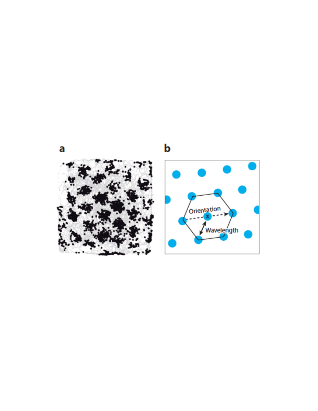
Electrical recordings of single neurons in the medial domain of the entorhinal cortex (MEC) of freely moving rodents have revealed spatially modulated neurons, called grid cells, firing action potentials only around the vertices of two dimensional hexagonal lattices covering the environment in which the animal navigates. The hexagonal firing pattern of a single grid cell is illustrated in the left panel of Figure 8. These grid cells can be categorized according to the orientation of their triangular grid, the wavelength (distance between the vertices ), and the phase (shift of the whole lattice). See the right panel of Figure 8 for an illustration of the orientation and wavelength of a single grid cell.
The data we analyze here consists of extra cellular recordings of several grid cells, and the simultaneously recorded location of the rat within a 300cm 300cm box for roughly 20 minutes66 6 The source of the data is [Stensola et al., 2012]. For a video of a single grid cell recorded in the MEC see the clip https://www.youtube.com/watch?v=i9GiLBXWAHI.. Since the number of spikes fired by a grid cell depends mainly on the location of the animal, regardless of the animal’s speed and running direction [Hafting et al., 2005], it is reasonable to summarize this spatial dependency in terms of a rate map , where is the expected number of spikes emitted by the grid cell in a fixed time interval , given that the animal is located at position during this time interval [Rahnama Rad and Paninski, 2010, Pnevmatikakis et al., 2014, Dunn et al., 2015]. In other words, if the rat passes the same location again, we again expect the grid cell to fire at more or less the same rate77 7 It is known that these rate maps can in some cases change with time but in most cases it is reasonable to assume them to be constant. Moreover, the two dimensional surface represented by is not the same for different grid cells., specifically according to a Poisson distribution with mean . For each grid cell, the estimation of the rate map is a first step toward understanding the cortical circuitry underlying spatial cognition [Rowland et al., 2016]. Consequently, the estimation of firing fields without contamination from measurement noise or bias from overs-smoothing will help to clarify important questions about neuronal algorithms underlying navigation in real and mental spaces [Buzsaki and Moser, 2013].
To be concrete, we discretize the two dimensional space into an grid, and discretize time into bins with width . In this example, is 0.4 seconds and is 50. The experiment is 1252.9 seconds long, and therefore we have time bins. In other words, . We use to denote the number of action potentials observed in time interval , where . Moreover, we use to denote a vector composed of zeros except for a single +1 at the entry corresponding to the animal’s location within the grid during the time interval . We assume a log-linear model , relating the firing rate at location to the latent vector where the latent spatial process responsible for the observed spiking activity is unraveled into . The firing rate can be written as . Due to this notation, is the value of at the animal’s location during the time interval . In this vein, the distribution of observed spiking activity can be written as
| (29) |

As mentioned earlier, the main goal is to estimate the two dimensional rate map , and a large body of work has addressed the problem of estimating a smooth rate map from neural data [DiMatteo et al., 2001, Gao et al., 2002, Kass et al., 2005, Cunningham et al., 2008, Czanner et al., 2008, Cunningham et al., 2009, Paninski et al., 2010, Rahnama Rad and Paninski, 2010, Macke et al., 2011, Pnevmatikakis et al., 2014]. Here we employ an over-complete basis to account for the spatially localized sensitivity of grid cells. Since it is known that the rate map of any single grid cell consists of bumps of elevated firing rates, located at various points in the two dimensional space, as illustrated in the left panel of Figure 8, it is reasonable to represent as a linear combination of , an over-complete basis in [Brown et al., 2001, Pnevmatikakis et al., 2014, Dunn et al., 2015]. We compose the over-complete basis using truncated Gaussian bumps with various scales, distributed at all pixels. The four basic Gaussian bumps we use are depicted in Figure 9. Since we use four truncated Gaussian bumps for each pixel, in this example, we have a total of basis functions. We employ the truncated Gaussian bumps where and are the horizontal and vertical coordinates. Define as a matrix composed of columns . Furthermore, define as , and define as a matrix composed of rows . We normalize the columns of , calling the resulting matrix . The columns of are unit normed. Formally, where is a diagonal matrix filled with the column-norms of . We use to refer to the rows of , yielding . Note that due to the above mentioned rescaling, we have the following relationship between the latent map and : . Sparsity of refers to our prior understanding that the rate map of a grid cells consists of bumps of elevated firing rates, located at various points in the two dimensional space, and therefore, our estimation problem is as follows:
Here we use the negative log-likelihood in equation (29) as the cost function, that is, . We remind the reader that we will use formula that was obtained in Theorem 1. Figures 10 illustrate that is reasonable approximation of , allowing computationally efficient tuning of . To see the effect of of the rate map, we also present the maps resulting from small and large values of , leading to under and over smooth rate maps, respectively. As it pertains to the reported run times, all fittings in this section were performed using the glmnet package [Qian et al., 2013] in MATLAB.

6 Concluding Remarks
Leave-one-out cross validation () is an intuitive and conceptually simple risk estimation technique. Despite its low bias in estimating the extra-sample prediction error, the high computational complexity of has limited its applications for high-dimensional problems. In this paper, by combining a single step of the Newton method with low-rank matrix identities, we obtained an approximate formula for , called . We showed how can be applied to popular non-differentiable regularizers, such as LASSO. With the aid of theoretical results and numerical experiments, we showed that offers a computationally efficient and statistically accurate estimate of the extra-sample prediction error in high-dimensions.
Important directions for future work involve various approximations that further reduce the computational complexity. The computational bottleneck of is the inversion of the large generalized hat matrix . This can make the application of to ultra high dimensional problems computationally challenging. Since the diagonals of our matrix can be represented as leverage scores of an augmented matrix, scalable methods to approximately compute the leverage score may offer a promising avenue for future work. For example [Drineas et al., 2012] offers a randomized method to estimate the leverage scores. However, the randomized algorithm presented in [Drineas et al., 2012] applies to the case, making it challenging to apply these methods to high-dimensional settings where is also very large. Nevertheless this is certainly a promising direction for speeding up .
In another line of work, the generalized cross-validation approach [Craven and Wahba, 1979, Golub et al., 1979] approximates the diagonal elements of with . Computationally efficient randomized estimates of can be produced without having any explicit calculations of this matrix [Deshpande and Girard, 1991, Wahba et al., 1995, Girard, 1998, Lin et al., 2000]. The theoretical study of the additional errors introduced by these randomized approximations, and the scalable implementations of them is another promising avenue for future work.
References
- [Akaike, 1974] Akaike, H. (1974). A new look at the statistical model identification. IEEE transactions on automatic control, 19(6):716–723.
- [Alison and Pillow, 2017] Alison, W. and Pillow, J. (2017). Capturing the dynamical repertoire of single neurons with generalized linear models. Neural Computation, 29(12):3260–3289.
- [Allen, 1974] Allen, D. (1974). The relationship between variable selection and data augmentation and a method for prediction. Technometrics, 16:125–127.
- [Bayati and Montanari, 2012] Bayati, M. and Montanari, A. (2012). The lasso risk for gaussian matrices. IEEE Transactions on Information Theory, 58(4):1997–2017.
- [Bean et al., 2013] Bean, D., Bickel, P. J., El Karoui, N., and Yu, B. (2013). Optimal m-estimation in high-dimensional regression. Proceedings of the National Academy of Sciences, 110(36):14563–14568.
- [Boucheron et al., 2013] Boucheron, S., Lugosi, G., and Massart, P. (2013). Concentration ineqaulities: A nonasymptotic theory of independence. Oxford University Press.
- [Boyd and Vandenberghe, 2004] Boyd, S. and Vandenberghe, L. (2004). Convex Optimization. Oxford University Press.
- [Breiman and Freedman, 1983] Breiman, L. and Freedman, D. (1983). How many variables should be entered in a regression equation? Journal of American Statistical Association, 78(381):131–136.
- [Brown et al., 2001] Brown, E., Nguyen, D., Frank, L., Wilson, M., and Solo, V. (2001). An analysis of neural receptive field plasticity by point process adaptive filtering. PNAS, 98:12261–12266.
- [Burman, 1990] Burman, P. (1990). Estimation of generalized additive models. Journal of Multivariate Analysis, 32:230–255.
- [Buzsaki and Moser, 2013] Buzsaki, G. and Moser, E. (2013). Memory, navigation and theta rythm in the hippocampal-entorhinal system. Nat Neurosci, 16(2):130–138.
- [Cawley and Talbot, 2008] Cawley, G. and Talbot, N. (2008). Efficient approximate leave-one-out cross-validation for kernel logistic regression. Machine Learning, 71:243–264.
- [Cessie and Houwelingen, 1992] Cessie, S. and Houwelingen, J. (1992). Ridge estimators in logistic regression. Applied Statistics, 41(1):191–201.
- [Craven and Wahba, 1979] Craven, P. and Wahba, G. (1979). Estimating the correct degree of smoothing by the method of generalized cross-validation. Numerische Mathematik, 31:377–403.
- [Cunningham et al., 2009] Cunningham, J., Gilja, V., Ryu, S., and Shenoy, K. (2009). Methods for estimating neural firing rates, and their application to brain-machine interface. Neural Networks, 22(9):1235–1246.
- [Cunningham et al., 2008] Cunningham, J., Yu, B., Shenoy, K., and Sahani, M. (2008). Inferring neural firing rates from spike trains using Gaussian processes. In Platt, J., Koller, D., Singer, Y., and Roweis, S., editors, Advances in Neural Information Processing Systems 20. Curran Associates, Inc.
- [Czanner et al., 2008] Czanner, G., Eden, U., Wirth, S., Yanike, M., Suzuki, W., and Brown, E. (2008). Analysis of between-trial and within-trial neural spiking dynamics. Journal of Neurophysiology, 99(5):2672–93.
- [Deshpande and Girard, 1991] Deshpande, L. and Girard, D. (1991). Fast computation of cross-validated robust Splines and other non-linear smoothing Splines. Curves and Surfaces, pages 143–148.
- [DiMatteo et al., 2001] DiMatteo, I., Genovese, C., and Kass, R. (2001). Bayesian curve fitting with free-knot splines. Biometrika, 88:1055–1073.
- [Dobriban and Wager, 2018] Dobriban, E. and Wager, S. (2018). High-dimensional asymptotics of prediction: Ridge regression and classification. Ann. Statist., 46(1):247–279.
- [Donoho et al., 2011] Donoho, D., Maleki, A., and Montanari, A. (2011). Noise sensitivity phase transition. IEEE Trans. Inform. Theory, 57(10).
- [Donoho and Montanari, 2016] Donoho, D. and Montanari, A. (2016). High dimensional robust m-estimation: Asymptotic variance via approximate message passing. Probab Theory Relat Fields, 166(3-4):935–969.
- [Donoho et al., 2009] Donoho, D. L., Maleki, A., and Montanari, A. (2009). Message passing algorithms for compressed sensing. Proc. Natl. Acad. Sci., 106(45):18914–18919.
- [Drineas et al., 2012] Drineas, P., Magdon-Ismail, M., Mahoney, M., and Woodruff, D. (2012). Fast approximation of matrix coherence and statistical leverage. Journal of Machine Learning Research, 13:3475–3506.
- [Dunn et al., 2015] Dunn, B., Morreaunet, M., and Roudi, Y. (2015). Correlations and functional connections in a population of grid cells. PLOS Computational Biology, 11(2):e1004052.
- [Efron, 1983] Efron, B. (1983). Estimating the error rate of a prediction rule: Improvement on cross-validation. JASA, 78(382):316–331.
- [Efron, 1986] Efron, B. (1986). How biased is the apparent error rate of a prediction rule? JASA, 81:461–470.
- [El Karoui, 2018] El Karoui, N. (2018). On the impact of predictor geometry on the performance on high-dimensional ridge-regularized generalized robust regression estimators. Probab. Theory Relat. Fields, 170:95–175.
- [El Karoui et al., 2013] El Karoui, N., Bean, D., Bickel, P., Lim, C., and Yu, B. (2013). On robust regression with high-dimensional predictors. PNAS, 110(36):14557–14562.
- [Frank and Friedman, 1993] Frank, I. and Friedman, J. (1993). A statistical view of some chemometric regression tools (with discussion). Technometrics, 35:109–148.
- [Friedman et al., 2010] Friedman, F., Hastie, T., and Tibshirani, R. (2010). Regularization paths for generalized linear models via coordinate descent. Journal of Statistical Software, 33(1):1–22.
- [Gao et al., 2002] Gao, Y., Black, M., Bienenstock, E., Shoham, S., and Donoghue, J. (2002). Probabilistic inference of arm motion from neural activity in motor cortex. In Thomas G. Dietterich, Suzanna Becker, Z. G., editor, Advances in Neural Information Processing Systems 14, pages 213–220.
- [Geisser, 1975] Geisser, S. (1975). The predictive sample reuse method with applications. Journal of American Statistical Association, 70(350):320–328.
- [Girard, 1998] Girard, D. (1998). Asymptotic comparison of (partial) cross-validation, GCV and randomized GCV in nonparametric regression. Ann. Statist., 26(1):315–334.
- [Golub et al., 1979] Golub, G., Heath, M., and Wahba, G. (1979). Generalized cross-validation as a method for choosing a good ridge parameter. Technometrics, 21(2):215–223.
- [Gorman and Sejnowski, 1988] Gorman, R. and Sejnowski, T. (1988). Analysis of hidden units in a layered network trained to classify sonar targets. Neural Networks, 1:75–89.
- [Gu, 1992] Gu, C. (1992). Cross-validating non-gaussian data. J. Comp. Graph. Stat., 1(2):169–179.
- [Gu and Xiang, 2001] Gu, C. and Xiang, D. (2001). Cross-validating non-gaussian data: Generalized approximate cross-validation revisited. J. Comp. Graph. Stat., 10(3):581–591.
- [Hafting et al., 2005] Hafting, T., Fyhn, M., Molden, S., Moser, M., and Moser, E. (2005). Microstructure of a spatial map in the enthorhinal cortex. Nature, 436:801–806.
- [He et al., 2018] He, L., Qin, W., Xu, P., and Zhou, Y. (2018). alocv: Approximate Leave-One-Out Risk Estimation. R package version 0.02.
- [Hurvich and Tsai, 1989] Hurvich, C. and Tsai, C. (1989). Regression and time series model selection in small samples. Biometrika, 76(2).
- [Kass et al., 2005] Kass, R. E., Ventura, V., and Brown, E. N. (2005). Statistical issues in the analysis of neuronal data. J Neurophysiol, 94:8–25.
- [Khan et al., 2014] Khan, U., Liu, L., Provenzano, F. A., Berman, D., Profacia, C., Sloa, R., Mayeux, R., Duff, K., and Small, S. (2014). Molecular drivers and cortical spread of lateral entorhinal cortex dysfunction in preclinical alzheimer’s disease. Nat. Neurosci., 17:304–311.
- [Leeb, 2008] Leeb, H. (2008). Evaluation and selection of models for out-of-sample prediction when the sample size is small relative to the complexity of the data-generating process. Bernoulli, pages 661–690.
- [Leeb, 2009] Leeb, H. (2009). Conditional predictive inference post model selection. Ann. Stat., 37(5B):2838–2876.
- [Lin et al., 2000] Lin, X., Wahba, G., Xiang, D., Gao, F., Klein, R., and Klein, B. (2000). Smoothing spline ANOVA models for large data sets with Bernoulli observations and the randomized GACV. Ann. Stat., 28(6):1570–1600.
- [Macke et al., 2011] Macke, J., Gerwinn, S., White, L., Kaschube, M., and Bethge, M. (2011). Gaussian process methods for estimating cortical maps. Neuroimage, 56(2):570–581.
- [Maleki, 2011] Maleki, A. (2011). Approximate message passing algorithm for compressed sensing. Stanford University PhD Thesis.
- [Mallows, 1973] Mallows, C. (1973). Some comments on . Technometrics, 15:661–675.
- [Meijer and Goeman, 2013] Meijer, R. and Goeman, J. (2013). Efficient approximate k-fold and leave-one-out cross-validation for ridge regression. Biometrical Journal, 55(2):141–155.
- [Moser et al., 2008] Moser, E., Kropff, E., and Moser, M. (2008). Place cells, grid cells, and the brain’s spatial representation system. Ann. Rev. Neurosci., 31:69–89.
- [Moser et al., 2014] Moser, E., Moser, M., and Roudi, Y. (2014). Network mechanisms of grid cells. Phil. Trans. R. Soc. B, 369(1635).
- [Mousavi et al., 2018] Mousavi, A., Maleki, A., Baraniuk, R. G., et al. (2018). Consistent parameter estimation for lasso and approximate message passing. The Annals of Statistics, 46(1):119–148.
- [Negahban et al., 2012] Negahban, S., Ravikumar, P., Wainwright, M., and Yu, B. (2012). High-dimensional generalized linear models and the lasso. Statistical Science, 4(27):538–557.
- [Nesterov, 2013] Nesterov, Y. (2013). Introductory lectures on convex optimization: A basic course, volume 87. Springer Science & Business Media.
- [Nevo and Ritov, 2016] Nevo, D. and Ritov, Y. (2016). On Bayesian robust regression with diverging number of predictors. Electron. J. Statist., 10(2):3045–3062.
- [Obuchi and Kabashima, 2016] Obuchi, T. and Kabashima, Y. (2016). Cross validation in lasso and its acceleration. J. Stat. Mech. Theor. Exp., 53(304):1–36.
- [Opper and Winther, 2000] Opper, M. and Winther, O. (2000). Gaussian processes and SVM: Mean field results and leave-one-out. In Smola, A., Bartlett, P., Scholkopf, B., and Schuurmans, D., editors, Advances Large Margin Classifiers, pages 43–56. MIT Press, Cambridge, MA.
- [O’Sullivan et al., 1986] O’Sullivan, F., Yandell, B., and Raynor, W. (1986). Automatic smoothing of regression functions in generalized linear models. JASA, 81(393):96–103.
- [Paninski, 2004] Paninski, L. (2004). Maximum likelihood estimation of cascade point-process neural encoding models. Network: Computation in Neural Systems, 15:243–262.
- [Paninski et al., 2010] Paninski, L., Ahmadian, Y., Ferreira, D., Koyama, S., Rahnama Rad, K., Vidne, M., Vogelstein, J., and Wu, W. (2010). A new look at state-space models for neural data. J. Comput. Neurosci., 29(0):107–126.
- [Park et al., 2014] Park, M., Weller, J., Horowitz, G., and Pillow, J. (2014). Bayesian active learning of neural firing rate maps with transformed Gaussian process priors. Neural Computation, 26:1519–1541.
- [Pillow, 2007] Pillow, J. (2007). Likelihood-based approaches to modeling the neural code. Bayesian brain: Probabilistic approaches to neural coding, pages 53–70.
- [Pnevmatikakis et al., 2014] Pnevmatikakis, E., Rahnama Rad, K., Huggins, J., and Paninski, L. (2014). Fast Kalman filtering and forward-backward smoothing via low-rank perturbative approach. J. Comp. Graph. Stat., 23(316-339).
- [Qian et al., 2013] Qian, J., Hastie, T., Friedman, J., Tibshirani, R., and Simon, N. (2013). Glmnet for Matlab.
- [Rahnama Rad and Paninski, 2010] Rahnama Rad, K. and Paninski, L. (2010). Efficient estimation of two-dimensional firing rate surfaces via Gaussian process methods. Computation in Neural Systems, 21:142–168.
- [Rowland et al., 2016] Rowland, D., Roudi, Y., Moser, M., and Moser, E. (2016). Ten years of grid cells. Ann. Rev. Neurosci., 39:19–40.
- [Schmidt et al., 2007] Schmidt, M., Fung, G., and Rosales, R. (2007). Fast optimization methods for l1 regularization: A comparative study and two new approaches. In ECML, pages 286–297. Springer.
- [Stein, 1981] Stein, C. (1981). Estimation of the mean of a multivariate normal. Ann. Stat., 9(6):1135–1151.
- [Stensola et al., 2012] Stensola, H., Stensola, T., Solstad, T., Froland, K., Moser, M., and Moser, E. (2012). The entorhinal grid map is discretized. Nature, 492(7427):72–80.
- [Stone, 1974] Stone, M. (1974). Cross-validatory choice and assesment of statistical predictions. J R Stat Soc Series B, 36(2):111–147.
- [Stone, 1977] Stone, M. (1977). An asymptotic equivalence of choice of model by cross-validation and akaike’s criterion. J R Stat Soc Series B, pages 44–47.
- [Su et al., 2017] Su, W., Bogdan, M., and Candes, E. (2017). False discoveries occur early on the Lasso path. Ann. Stat., 45(5):2133–2150.
- [Tibshirani, 1996] Tibshirani, R. (1996). Regression shrinkage and selection via the lasso. Journal of the Royal Statistical Society. Series B, 58:267–288.
- [Tibshirani and Taylor, 2012] Tibshirani, R. and Taylor, J. (2012). Degrees of freedom in lasso problems. Annals of Statistics, 40(2):1198–1232.
- [Tibshirani et al., 2013] Tibshirani, R. J. et al. (2013). The lasso problem and uniqueness. Electronic Journal of Statistics, 7:1456–1490.
- [Van de Geer, 2008] Van de Geer, S. (2008). High-dimensional generalized linear models and the lasso. The Annals of Statistics, 2(36):614–645.
- [Van der Vaart, 2000] Van der Vaart, A. W. (2000). Asymptotic statistics, volume 3. Cambridge university press.
- [Vehtari et al., 2017] Vehtari, A., Gelman, A., and Gabry, J. (2017). High-dimensional generalized linear models and the lasso. Statistics and Computing, 5(27):1413–1432.
- [Vehtari et al., 2016] Vehtari, A., Mononen, T., Tolvanen, V., Sivula, T., and Winther, O. (2016). Bayesian leave-one-out cross-validation approximations for Gaussian latent variable models. Journal of Machine Learning Research, 17(1):3581–3618.
- [Wahba et al., 1995] Wahba, G., Johnson, D., Gao, F., and Gong, J. (1995). Adaptive tuning of numerical weather prediction models: Randomized GCV in three- and four-dimensionalassimilation. Monthly Weather Review, 123:3358–3369.
- [Wainwright, 2009] Wainwright, M. (2009). Sharp thresholds for high-dimensional and noisy sparsity recovery using -constrained quadratic programming (lasso). IEEE Trans. Inf. Theory, 55(5):2183–2202.
- [Weng et al., 2018] Weng, H., Maleki, A., and Zheng, L. (2018). Overcoming the limitations of phase transition by higher order analysis of regularization techniques. Annals of Statistics.
- [Xiang and Wahba, 1996] Xiang, D. and Wahba, G. (1996). A generalized approximate cross validation for smoothing splines with non-gaussian data. Statistica Sinica, 6:675–692.
- [Zolrowski and Pillow, 2018] Zolrowski, D. and Pillow, J. (2018). Scaling the Poisson GLM to massive neural datasets through polynomial approximations. Advances in Neural Information Processing Systems, pages 3517–3527.
- [Zou and Hastie, 2005] Zou, H. and Hastie, T. (2005). Regularization and variable selection via the elastic net. J. R. Statist. Soc. B., 67(2):301–320.
- [Zou et al., 2007] Zou, H., Hastie, T., and Tibshirani, R. (2007). On the “degrees of freedom” of the lasso. Ann. Stat., 35(5):2173–2192.
Appendix A Proofs (FOR ON-LINE PUBLICATION ONLY)
A.1 Several concentration results for Gaussian random vectors and matrices
In this section, we mention a few concentration results that will be used multiple times in the proofs of our main results. We standard and well-known Gaussian tail bound:
Lemma 10.
Let . Further assume that . Then,
Our next lemma obtains a tail bound for the magnitude of a Gaussian random vector and the maximum eigenvalue of a Gaussian matrix.
Lemma 11 (Due to [Boucheron et al., 2013]).
Let with , where then
| (30) |
Furthermore, if is composed of independently distributed entries, then
| (31) |
The above lemma shows how we can find a tail bound for the maximum singular value of an iid Gaussian matrix. Below we extend the result to Gaussian matrices whose columns are dependent on each other. Note that Lemma 12 is the same as Lemma 5 with and . Hence we present the proof Lemma 12 which can be easily used to prove Lemma 5.
Lemma 12.
is composed of independently distributed rows, with , where then
| (32) |
A.2 Proof of Theorem 1
A.2.1 Roadmap of the proof
We first remind the reader that . Before we discuss the proof, let us mention the following definitions:
| (35) | |||||
| (36) |
Note that according to Assumptions 1 and 2, and are unique. We first mention a few structural properties of that will be used throughout our proof. Since the proofs of these results are straightforward, we skip them.
Lemma 13.
For any we have , and
In particular, as , uniformly converges to .
Lemma 14.
is infinitely many times differentiable, and
| (37) |
Furthermore, if for a constant , then . Finally, if for a constant , then and .
Now, we show the main steps for finding the following limit
In that vein, let
| (38) |
where . Based on Theorem 4 in Section A.2.3, for large enough , there exist fixed numbers such that
which with Lemma 14 implies for and for , as . Since the diagonal elements of go off to infinity, , as . Furthermore, since the diagonal elements of converge to zero, . Therefore, by using the following identity
| (39) |
and noting that , , we obtain
A.2.2 Proof of
Suppose that does not go to zero as . Then, there exists an for which we can find a sequence such that
| (42) |
According to Lemma 13, we have
| (43) |
Note that Inequality (a) uses Lemma 13 which proves . Inequality (b) is due to the fact that and we assume that the loss function returns positive numbers. Inequality (c) is due to the fact that is the minimizer of .
According to (43) the sequence belongs to a compact set, and hence has a converging subsequence, called . Suppose that converges to . Therefore,
| (44) |
Inequality (d) is due to (40). Inequality (e) is true because is the minimizer of , and finally Inequality (f) is due to (41). By taking the limit from both sides of (44), we have
But is different from , according to (42), contradicting the uniqueness of in Assumption 1. .
A.2.3 Bounds for regression coefficients in smoothed LASSO
Theorem 4.
Proof. The optimality conditions
| (45) | |||||
| (46) |
lead to
| (47) |
We know from Lemma 15. And since is twice differentiable (Assumption 3), we can argue that as . Hence,
| (48) |
as . This shows that for every , should remain bounded as . Suppose that this is not true. Then we find a subsequence that as . Then
If we combine this with Assumption 4, we conclude that will be a constant due to the assumption . This is in contradiction with (48). Hence, we have proved that for every , remains bounded.
Next, we show that is bounded away from zero in the limit . Define . Lemma 15 implies , and therefore, for large enough, we have
leading to
A.3 Proof of Theorem 2
The following lemma plays a critical role in our proof of Theorem 2.
Lemma 16.
Consider a class of symmetric positive definite matrices of the form
| (49) |
where , and . Then, for any vector we have
Furthermore, if we define , then .
Proof: Define . Note that since the matrix is always positive definite, for any value of , . By using the formulas for the inverse of block matrices we have
| (50) |
Define .
| (51) | |||||
Lemma 16 follows from the monotonicity of in terms of .
Proof of Theorem 2.
Before we start the proof, let us emphasize on the following facts that will be used later in the proof.
- 1.
- 2.
Consider . Then by definition . Similar to the proof of Theorem 1, we have as .
Hence, we already know the limiting behavior of for and as . The only remaining index set is . Unfortunately, for we can not specify the limiting behavior of . Hence, our goal is to use Lemma 16 to get around this issue. Set and define the matrices
| (52) |
Given this notation we have
| (53) |
Here each element of may converge to any number in the range . Hence we use Lemma 16 to find upper and lower bounds for . According to Lemma 16 we have
| (54) |
and
| (55) | |||||
The rest of the proof is similar to the proof of Theorem 1; we take the limit from both sides of (54) and (55), and then use the block matrix inversion formulas (similar to those used in the proof of Theorem 1) and the fact that as to complete the proof. ∎
A.4 Derivation of (18)
A.4.1 Roadmap of the derivations
The goal of this section is to derive the formula, presented in (18), for the following class of bridge estimators:
| (56) |
where . Since is not twice differentiable at zero, similar to what we did for LASSO, we first consider a smoothed version of the bridge regularizer:
| (57) |
where satisfies the following conditions:
- (i)
-
has a compact support, i.e., . Also, for every .
- (ii)
-
and ;
- (iii)
-
is infinitely many times smooth and symmetric around 0 on ;
The two important properties of are
- 1.
is infinitely many times differentiable for any nonzero value of .
- 2.
as . This claim will be proved in Lemma 17 below.
Hence, instead of finding the formula directly for (56), we start with
| (58) |
Given that both the loss function and the regularizer are smooth in (58), we can use (6) to obtain the following formula as the estimate of the out-of-sample prediction error of :
| (59) |
where
| (60) |
Note that we are interested in for large values of . Hence, as suggested for the LASSO problem in Section 2.2, we calculate . In Section A.4.3 we prove the following theorem:
Theorem 5.
If the loss function is twice continuously differentiable with respect to its second argument, and the optimization problem in (58) has a unique solution for every , then
| (61) |
where
| (62) |
is the active set of , and .
A.4.2 Basic properties of
Lemma 17.
The smoothed regularizer satisfies
Proof.
According to the symmetry, we only consider . We have
| (63) | |||||
Note that inequality (a) is due to the fact that since , the difference between is maximized when . In other words,
Furthermore, equality (b) is a result of the mean value theorem and . ∎
A.4.3 Proof of Theorem 5
Consider the following definitions:
| (64) |
As discussed in Lemma 17, the difference is bounded by the maximum value that takes. Our first lemma shows that . Hence, according to Lemma 17 the discrepancy between goes to zero as .
Lemma 18.
There exists an such that and .
Here we only present the sketch of the proof, and skip the straightforward details. If , then . Hence, since is bounded, cannot go off to infinity. We can now use this lemma to prove that as , .
Lemma 19.
If the optimization problems in (64) have unique solutions, then as
The proof of this lemma is similar to the proof of Lemma 15, and is hence skipped here. As mentioned in Section A.4.1, the main step in proving Theorem 5 is to find the limit of . The main step in this calculation is to calculate . The following lemma shows how this limit can be calculated.
Lemma 20.
Let denote a function of . If as , then
Proof.
Without loss of generality we consider the case . We consider three different cases. Each case has a slightly different proof strategy.
- 1.
Case I: or .
- 2.
Case II: , where .
- 3.
Case III: .
It is straightforward to show that
| (65) |
Note that for outside the interval . Now we consider the three cases we described above.
Case I: We assume that for large enough values of , . Clearly, this holds when . However, it may be violated when . But, this special case can be handled with a similar approach and is hence skipped. We have
| (66) | |||||
Equality (a) is due to the mean-value theorem. To obtain (b) we used the fact that , and that (hence ). The last equality is the result of integration by parts. Note that since as , .
Case II: , where . For large enough values of , we know that . Hence, according to (65) we have
| (67) | |||||
It is straightforward to confirm that .
Case III: First note that since , for large enough , . Similar to the derivation in (67), we have
| (68) | |||||
Again, it is straightforward to see that the last expression goes to as . ∎
We remind the reader that our goal is to show that
where denotes the active set of . Since, , and and functions are continuous, it is straightforward to prove that
Let denote the set of indices of the non-zero elements of , and define
| (69) |
Also define . According to Lemmas 19 and 20, the diagonal elements of go off to infinity. Hence, it is straightforward to show that , as . By using the following identity
| (70) |
and noting that , , and we obtain
A.5 Proofs of the Lemmas of Section 4
A.5.1 Proof of Lemma 3
Since
using simple algebra it is straightforward to show that for any , we have
Therefore,
Finally, based on the inequality above, we have
The last statement of the Theorem is a direct result of Lemma 12.
A.5.2 Proof of Lemma 8
Since
where
| (71) |
Concerning equations (71), the following inequalities hold
For any , consider the function
It is straightforward to check that is a decreasing function of and that . Hence, by simply using , for any , we have
Moreover,
Since
Therefore, , leading to
Finally, based on the inequality above, we have
A.5.3 Proof of Lemma 9
We prove Lemma 9 using the following inequality (for large enough such that )
where Note that according to Lemma 12, we have
In the next step, we bound . We have
| (72) |
For , set . We have
where (a) is a result of Markov’s inequality, and (b) uses the formula for the moment generating function of a Poisson random variable. It is straightforward to see that . Hence,
If we set , then (for large enough such that ) we will have
Define the event
and the set
First note that
If we define the event
then , leading to
Note that (for large enough )
| (73) | |||||
where (c) is a direct consequence of the Gaussian tail bound in Lemma 10 and the fact that . Furthermore, if , then
| (74) |
We now have
| (75) | |||||
where .
A.5.4 Proof of Lemma 4
Note that
| (76) |
Note that . To see this consider the following two cases:
-
Case I, :
-
Case II, :
Therefore,
Finally, based on the inequality above, we have
A.5.5 Proof of Lemma 7
Define
| (77) |
Furthermore, define . Since , where , the optimality conditions yield
| (78) | |||||
We bound and complete the proof of Lemma 7, by separately bounding the infinity norm of each of the three terms in 78 using Lemma 21, 22 and 23, and defining
| (79) |
where is introduced in Lemma 23.
Lemma 21.
Under the assumptions of Lemma 7 we have
Proof.
First note that
| (80) |
Define . According to the matrix inversion lemma we have
| (81) |
Note that conditioned on the distribution of is a zero mean Gaussian random variable with variance . Hence, (81) and the Gaussian tail bound, i.e. Lemma 10, lead to
| (82) |
Hence, by marginalizing , we get
By setting we have
This combined with a union bound and (80) proves that
∎
Lemma 22.
If , then
Proof.
Note that conditioned on , the distribution of is multivariate Gaussian with mean zero and covariance matrix . We have
| (83) |
We define . Clearly , hence,
| (84) |
Hence, by setting , we have
∎
Lemma 23.
Proof.
Since , we have
| (87) |
Furthermore, due to , (see Lemma 14), and (87), we have
| (88) |
The first order optimality condition yields
Since the minimum eigenvalue of the Hessian of is , therefore the minimum eigenvalue of (for all ) is greater than , leading to
This together with yields
Define . According to the matrix inversion lemma we have
| (89) |
Furthermore, we have
| (90) |
First note that, since the maximum eigenvalue of is we have
| (91) | |||||
Furthermore, we have
| (98) | |||||
Next, we compute an upper bound on . Since is independent of and , we conclude that given and , is a Gaussian random variable with mean zero and variance
where , and the second inequality is due to (88). Hence,
Considering the event of , we have
| (99) |
Hence,
| (100) |
By combining (89), (90), (98), and 100 we conclude that if
then
| (101) | |||||
Hence,
∎
A.5.6 Proof of Lemma 2
Since , we have , and because of Lemma 13, . Moreover, . The next step is
A.6 Proof of Theorem 3
Lemma 24.
Let be a matrix with . Moreover, let and be diagonal matrices with positive elements, then
where .
Lemma 25.
Assume that and are positive definite, and define:
| (102) | |||||
| (103) | |||||
| (104) | |||||
| (105) |
Then,
| (106) |
Lemma 26.
Lemma 27.
Let with , where then
| (107) |
Moreover, if
| (108) | |||||
| (109) |
where is independent of the symmetric matrix and , then
| (110) | |||||
| (111) |
Proof of Theorem 3.
Let denote the event that (22), (23), (24), and (25) hold. Furthermore, define the following events:
| (112) | |||||
| (113) | |||||
| (114) | |||||
| (115) | |||||
| (116) | |||||
| (117) |
where in (113) is a positive constant (defined later in (123)), and
| (118) | |||||
| (119) | |||||
| (120) |
The variable in (118) is later set to 3, but for now all we need to know is that it is a positive constant. Due to Lemma 26, if the event holds, then for every we have
Since , we have
| (121) | |||||
Hence, we now obtain an upper bound for ;
| (122) | |||||
where is due to Inequality (111) from Lemma 27. To bound we define
| (123) | |||||
obtained by setting , and computing after putting and , bounds in event , into and , respectively. Next,
The term is exponentially small because is with , leading to
| (124) |
due to Lemma 11 and Lemma 12. In summary, since for we have , for we obtain
This combined with (121) leas to
| (125) | |||||
where the last inequality is due to the assumption that . Hence, Inequality (26) in Theorem 3 follows. Note that in the presentation of Theorem 3, we replaced respectively and with the upper-bounds 72 and 5, and we replaced with the upper bound . We also used to denote .
∎
A.7 Proofs of lemmas 24, 25, 26, 27 and 12
Proof of Lemma 24.
Let . Moreover, let stand for the sub-matrix of restricted to the rows indexed by , and let be the diagonal matrix with the diagonal elements of indexed by . Then, , and in turn, the Woodbury inversion lemma yields
| (126) | |||||
Using the Woodbury lemma again we obtain
| (127) | |||||
Hence, by using (126) and (127) we have
∎
Proof of Lemma 25.
Proof of Lemma 26.
Define the approximate leave--out perturbation vector as
| (129) |
where the exact leave--out perturbation vector is given by
| (130) |
Woodbury lemma yields:
| (131) | |||||
where . Define
| (132) |
The leave-one-out estimate, , satisfies . The multivariate mean-value Theorem yields
| (133) |
where the Jacobean is
| (134) |
Moreover, satisfies
We get
so that
| (135) |
leading to the following inequality
| (136) |
as a consequence of Assumption 7. Next, we look at the part of dependent on , so we rewrite (135) as
| (137) |
Let us rewrite the Jacobean in a more compact form:
| (138) |
where
| (139) |
Define
| (140) |
so that
| (141) |
Note that is positive definite for all , and , due to Assumption 7. The last steps of the proof are as follows:
where
-
is due (141).
-
is due the fact that for any we have ,
-
is due to Assumption 6 as illustrated below
Likewise,
(142) Here we should emphasize that this is the main place in which we have used the smoothness of second derivatives of the loss and regularizer in Assumption 6. 88 8 Note that by checking the derivation, it is clear that we can replace Assumption 6 with the following weaker assumptions: (143) (144) for some , and still find an (weaker) upper bound for that converges to zero as .
-
is due to (139), and
(145)
The final result follows the basic inequality: . ∎
Proof of Lemma 27.
First, we prove
| (146) |
as follows