A Single-Planner Approach to Multi-Modal Humanoid Mobility
Abstract
In this work, we present an approach to planning for humanoid mobility. Humanoid mobility is a challenging problem, as the configuration space for a humanoid robot is intractably large, especially if the robot is capable of performing many types of locomotion. For example, a humanoid robot may be able to perform such tasks as bipedal walking, crawling, and climbing. Our approach is to plan for all these tasks within a single search process. This allows the search to reason about all the capabilities of the robot at any point, and to derive the complete solution such that the plan is guaranteed to be feasible. A key observation is that we often can roughly decompose a mobility task into a sequence of smaller tasks, and focus planning efforts to reason over much smaller search spaces. To this end, we leverage the results of a recently developed framework for planning with adaptive dimensionality, and incorporate the capabilities of available controllers directly into the planning process. The resulting planner can also be run in an interleaved fashion alongside execution so that time spent idle is much reduced.
I Introduction
Recent years have shown much interest in developing robust humanoid robots that can operate in environments that are often unstructured, cluttered, and unpredictable compared to controlled industrial settings. Furthermore, the structure that does exist is intended primarily for people, and not designed with the robots in mind. Structures such as staircases, ladders, railings, complement people’s mobility. This leads us to design humanoids so that they possess capabilities similar to people such as the ability to walk, climb, and use surfaces such as handrails for support.
The need for all these capabilities provides a number of challenge problems for motion planning. The most pronounced problem is the inherent high dimensionality of the robot’s configuration space. To guarantee that a plan safely and efficiently accomplishes a given task may require reasoning about all of the joints of the robot and the relationship between the robot and the various objects in its environment. These constraints are expensive to evaluate.
Luckily, a complicated mobility task can often be broken down into a sequence of smaller tasks. For example, a task for a robot to move from one end of a facility to the other might include traversing large areas by walking, climbing staircases or ladders and, in situations where the environments is hazardous, crawling under fallen structures or over debris. Examples of such environments are shown in Figure 1.


Typically, current approaches solve this problem hierarchically: a top-level planner decomposes the complete task into smaller tasks and then runs a different planner, specialized for the each task, in isolation. Once plans are computed for each task, the top-level planner figures out how the robot will transition from one task to the next. This can be done with yet another specialized planner, or prescripted behaviors. The results of the Darpa Robotics Challenge, as demonstrated in [1], [2], [3], show the ubiquity of specialized task planners and behaviors. This common approach has shown to be brittle, as each task planner is constrained to satisfy the requirements of the original task decomposition, and must satisfy strict endpoint constraints to ensure that the transitions between tasks are feasible. In the worst case, where the top- level planner has chosen an incorrect decomposition, one of the planners may be unable to generate a solution at all or a transition between tasks is infeasible.
The approach presented here builds upon the notion of adaptive dimensionality. Rather than always search through a high-dimensional state space, adaptive dimensionality automatically figures out what dimensions are relevant in each region of the state space. This is tremendously beneficial to planning for humanoid mobility as there is lots of redundant motion that makes up the various modes of locomotion available to them. This paper presents how adaptive dimensionality can be applied to humanoid mobility, describes an implementation that yields real-time execution by interleaving planning and execution, and presents experimental results showing the practicality of the approach.
II Related Work
Much work in humanoid mobility planning is focused on solving specific sub-problems of mobility. Examples of navigation planning using footsteps are shown in [4], [5]. These techniques plan in a low-dimensional space representing feasible footstep actions. They may rely on a controller to produce feasible joint trajectories or the planner may generate these trajectories online to ensure footstep validity. Example whole-body planning techniques have been explored in [6], [7], [8]. These approaches are generally intended for object interaction tasks, and don’t consider incorporating locomotion. Some example techniques specifically for climbing ladders are presented in [9] and [10].
Relatively less work has been done for humanoid robots on adaptively reasoning about the relevant dimensionality of the problem during the search process. Some examples of adaptive reasoning include [11] and [12]. Both works decompose the robot into appropriate subsystems based on kinematics, increase the dimensionality. The first RRT-based approach adaptively adds subsystems as the search gets closer to the goal. The second, optimization-based approach, plans iteratively, incorporating more descendant subsystems until a valid path is found. These approaches both iteratively increase the dimensionality of the entire search space, whereas our approach only increases dimensionality of the search space in regions where high-dimensional planning is required.
III Planning Framework
Our application to multi-modal humanoid navigation targets the humanoid robot shown in Figure 3. The robot has 4 symmetric limbs, each with 7 degrees of freedom, and additional joints for reorienting the attached sensors. At the end of each limb, is a dual-purpose end effector designed with a flat surface, both for walking and support, and a hook for latching onto cylindrical-shaped objects in the environment, such as ladder rungs and handrails. In this work, we explicitly plan for all of the joint variables of the limbs. The pose of the robot provides an additional 6 degrees of freedom for its global position and orientation. Together these degrees of freedom define a 34-dimensional search space.
We are also provided with a set of specialized controllers for performing various locomotion tasks. Currently, the robot is equipped with controllers for bipedal walking, crawling, and climbing ladders. Additionally, we are able to directly control each of the joint actuators to execute raw full-body paths. While it is possible to plan paths consisting of only raw joint motion, we are able to leverage the existence of the controllers both to improve planning efficiency and generate plans that can be executed more robustly on the actual robot.
We represent the planning problem as a search over a finite, discrete search space. The search space consists of a discrete state space , and a set of transitions . Each pair represents a feasible transition between two states. Each transition is associated with a scalar cost, . We use the notation to denote a path from state to state , and to denote an optimal, least-cost, path. This search space defines a graph , with vertex set and edge set . The goal of the planner is to find a path in from a given start state to a goal state , where .
To improve the efficiency of the search through this high-dimensional space, and to ease integration of specialized controllers, our algorithm takes much of its inspiration from the Planning with Adaptive Dimensionality framework presented in [13] and [14]. The framework for planning with adaptive dimensionality makes the observation that, in many areas of the search space, it is often not necessary to reason about the high dimensionality of the state space, as many of the resulting paths have a low-dimensional structure.
Section IV will begin with a brief overview of the framework for planning with adaptive dimensionality. Section V will describe extensions to the planning with adaptive dimensionality framework to enable planning with multiple low-dimensional planning representations simultaneously. Section VII will describe the details of the search algorithm used during the first phase of a single search iteration, with an emphasis on the use of multi-heuristic search. Section VIII will describe the details of the search algorithm used during the second phase of a single search iteration, with an emphasis on incorporating user demonstrations to accelerate planning similar transitions in the high-dimensional space. Section IX will describe how the search can be run in a resumable fashion to enable interleaving of planning and execution. Section X will present a brief overview of the control architecture on the robotic platform, and specifically how plans are delivered to the appropriate controllers during execution. Section XI will list the results of sample runs of the planner on targeted test environments.
IV Planning with Adaptive Dimensionality
This section provides a brief overview of the framework for planning with adaptive dimensionality. For detailed analysis of the adaptive dimensionality framework and additional applications, see [13].
For a complete planning solution, a search often needs to reason over a high-dimensional state space. However, we expect that large portions of a complete plan will exhibit a low-dimensional structure. For example, part of a humanoid mobility task might include large segments of bipedal walking. In these scenarios, it suffices to plan only for the footstep locations, and we reserve planning in the high-dimensional space for verifying that each footstep is feasible. The portions of the plan requiring high-dimensional reasoning are infrequent compared to portions that can be solved in this manner.
The planning with adaptive dimensionality framework leverages this low-dimensional structure by iteratively constructing a hybrid search space, composed primarily of low-dimensional states and transitions, and introducing high-dimensional states and transitions where necessary to ensure feasibility of the resulting path.
IV-A Graph Structure
The adaptive dimensionality framework considers two state spaces: the original high degree-of-freedom state space that represents valid configurations of the robot, and a projection of the original state space to a low-dimensional representation, respectively labeled and . A many-to-one mapping defined by
represents the projection from the high-dimensional space to the low-dimensional space. The inverse, one-to-many, mapping defined by
represents the projection from a state in the low-dimensional space back to a subset of states in the high-dimensional space.
Both the high-dimensional and low-dimensional space can have its own set of transitions, and respectively. However, to guarantee completeness and bounded suboptimality, the following constraint is required:
| (1) |
That is, the cost of the optimal path between any two states in the high-dimensional space must be at least the cost of the optimal path between their projections in the low-dimensional space.
The notation and represent the corresponding high-dimensional and low-dimensional graphs defined as and , respectively.
IV-B Search Algorithm
Rather than search for a path in the original high-dimensional search space, , the adaptive dimensionality search algorithm prefers to search as much as possible in the low-dimensional search space, . To accomplish this, the search iteratively constructs a new hybrid search space , composed of an adaptive state space , and transition set . This new search space is composed primarily of states and transitions from and is expanded to include regions of states and transitions from as necessary.
Initially, the adaptive search space includes all of . When a region of high-dimensional states is introduced, is updated so that low-dimensional states that fall within the high-dimensional region are replaced by their high-dimensional equivalents in .
To be able to search this hybrid space, we must define a transition set that includes transitions between states from and . The transition set for the adaptive search space is defined as follows. For a state ,
- •
If then for all transitions , if then otherwise
- •
If then for all transitions , if then . Additionally, for all transitions , where , if then
This transition set includes transitions between low- and high-dimensional states, and only includes transitions to states in the adaptive state space . Notice that expanding or adding a new high-dimensional produces a new instance of .
The adaptive search algorithm begins by finding a path, , from the start to the goal in the current instance of . This path is allowed to contain states of differing dimensionalities, and so may not be executable. If no path is found during this phase, then no path exists from the start to the goal, and the search terminates. To construct an executable path from , another search is conducted within a tunnel surrounding . We define a tunnel of radius around an adaptively-dimensional path as follows: is a subgraph of . A high-dimensional state if there exists a state such that the distance from to (or if ) is no larger than for some pre-defined distance metric on . All transitions are included such that .
If the search fails to find a path from the start to the goal within , high-dimensional regions are introduced where the search became stuck, and the adaptive search begins a new iteration on a newly constructed instance of . See [13] for details on how to identify locations to place high-dimensional regions.
V Adaptive Dimensionality with Multiple Low-Dimensional Representations
In the domain of humanoid mobility planning, several useful low-dimensional representations are available. For our application, the humanoid robot is expected to utilize the available controllers for optimized bipedal walking, crawling, and ladder climbing. Each of these controllers has a natural low-dimensional representation. For crawling, the controller requires a 4-dimensional pose, , of the robot. For bipedal walking, the controller requires paths that specify the 4-dimensional pose, , of each foot. Finally, for ladder climbing, the controller requires only the 6-dimensional pose, , for each of the four end-effectors. To be able to plan solutions that incorporate all of these representations, we need the ability to combine into a single search space.

Our approach maintains the separation between the high-dimensional and low-dimensional search spaces and their ability to define their own transition sets. Given low-dimensional representations, we define low-dimensional discrete state spaces , and their corresponding transition sets, .
The mappings from the high-dimensional space to each low-dimensional space remain largely unchanged as well. For the ’th low-dimensional representation, a mapping defined by
represents the mapping from states in to states in . Correspondingly, the inverse functions
represent the mapping from states in to subsets of .
Additionally, we define functions
to represent the mappings between states of low-dimensional representations. These mappings may be one-to-one or one-to-many depending on the dimensionality of the target representation.
The construction of , and its graph representation, , follows from its construction in the adaptive dimensionality framework. The initial instance of is the union of the search spaces for each of the low-dimensional representations. The transition set, is extended to include projections from the high-dimensional representation to each low-dimensional representation. Additionally, also contains transitions that allow the search to effectively switch between low-dimensional representations. The complete transition set is defined as follows. For a state ,
- •
If then, for all high-dimensional transitions , if then , otherwise for each low-dimensional representation
- •
If then, for all low-dimensional transitions , if then . Additionally, for each representation , for all transitions , where , if then
Thus far, we have only described how to incorporate multiple low-dimensional representations into the adaptive dimensionality framework. This indeed speeds up the search for finding a high-dimensional path, but we also desire to explicitly reason about the controller capabilities, to avoid high-dimensional planning wherever possible. Recall that during the second phase of each search iteration, the algorithm searches for a completely high-dimensional path, within the tunnel . To relieve the search of needing to perform high-dimensional planning, we extend the transition set of the high-dimensional representation to include all of the transitions that correspond to actions from the low-dimensional representations that are directly executable by an available controller.
VI Low-Dimensional Representations for Humanoid Mobility
In this domain, the high-dimensional state space represents all the controllable degrees of freedom of the robot. Each low-dimensional state space represents one of the available modes of locomotion. These low-dimensional representations are depicted in Figure 3.


A state vector for the full-body state space contains a single discrete variable for each actuated joint, plus 6 variables for the pose of the robot. Combined, a state vector for the full-body state space is represented as
Each discrete variable corresponds to a range of continuous values, obtained by simple discretization functions. The discretization resolution was chosen as for all translational variables, and as for all rotational variables. The action space is built from several types of motion primitives. The first type directly moves each joint of the robot individually by some small delta. We chose simple motion primitives that varied each joint by the state space discretization of . The second type of motion primitive uses an inverse kinematics solver to move the position of one of the end effectors by a small positional delta. We chose simple primitives to move an individual end effector by in x, y, or z. Finally, we allow full-body IK motions for the root of the robot. The root is allowed to move in x, y, or z by or yaw by , , or . Since there were no controllable degrees of freedom between the root of the robot and the base of each limb, our full-body body IK solver simply runs an isolated IK solver for each of the limbs that are currently supporting the weight of the robot. The last type of motion primitive is an adaptive motion primitive that computes the motion, on-the-fly, that achieves a selected target for one of the limbs. These targets are selected according to nearby support surfaces, such as the ground or handrails.
The representation for bipedal walking contains state vectors describing the 4-dimensional poses of each of the foot, plus one extra variable for restricting the gait of the robot to a left-right alternating scheme. The combined state vector is represented as
where is or to denote the pivot foot. We restrict the actions allowed in the bipedal state representation to a fixed set of target poses, offset from the current pivot foot. Application of one of these actions places the opposite, active foot with respect to the pivot foot. We included total primitives: of these allow reorienting of the feet to produce turning motions, and the remaining move the feet forward at varying distances from to to trade off between state space coverage and allowing the search to quickly explore long distances via forward walking.
The representation for crawling contains state vectors describing a four-dimensional pose for the center-of-mass of the robot. We include a simple set of actions that allow the robot to move directly forward or backward by , and to turn-in-place by , to mimic the capabilities of the controller.
The representation for ladder climbing contains state vectors describing a six-dimensional positions for each of the robot’s end effectors. Each action moves all four end effectors from their current positions to positions on the ladder rung directly above or below the currently held rung, as indicated by the current end effector positions.
The projection functions, from the full-body representation to each of these low-dimensional representations require solving forward kinematics for the given full-body state. The inverse projections from each low-dimensional representation to the high-dimensional representation require expensive inverse kinematics queries to determine valid configurations for the robot. To accelerate this process, we precompute a small set of nominal joint configurations for the full-body state, and perform small searches for a nearby valid configuration. Conveniently, these nominal joint configurations also correspond to the joint configurations we can expect the robot to achieve after execution of one of the controllers.
Notice that because of the restrictions on the available actions for each state representation, the planner may be unable to discover relevant projections between the state representations. To aid the planner, we append special transitions, whose resulting successor states project cleanly to another state representation. For example, a successor state for bipedal is generated such that the feet end up on a ladder rung, so that the resulting projection is relevant to the ladder representation. We designed similar transitions from bipedal to crawling and from crawling to ladder. These special successor states are only for projections to other representations, and may not produce successor states of their own.
By design, the available actions in the crawling and ladder representations are always directly executable by an existing controller. However, the bipedal representation contains actions that are not directly executable. For example, the bipedal representation is allowed to make footsteps that traverse up and down staircases, while the available controller is only allowed to operate on even terrain. These non-executable actions are resolved during the second phase of the search by planning in the high-dimensional space.
VII MR-MHA*
In this section we describe a planning algorithm which is better suited to planning in multiple representation state-spaces. This algorithm, called the MultiRep-MultiHeuristic A* (MR-MHA*), is a generalization of the MHA* algorithm [15] that can reason over several different state-space representations, each of which may have its own heuristics defined.
Multi-Heuristic A* is a search framework that uses multiple inadmissible heuristics to simultaneously explore the search space, while preserving guarantees of completeness and suboptimality bounds by using a single admissible ”anchor” heuristic. The algorithm has shown success in complex high-dimensional planning problems such as mobile manipulation planning for the 12D PR2 robot, where a naive weighted-A* approach is sensitive to large local minima. Two variants of MHA* are described in [15]. In this work we simply refer to the shared variant SMHA* as MHA*.
As mentioned earlier, humanoid mobility presents several low-dimensional representations like bipedal walking, ladder climbing etc. It would be preferable for the search to explore along both the ladder and stairway at the same time to reach the goal. Also since these low-dimensional representations are complex enough and fundamentally different, we might need different heuristics to explore each representation. This is the motivation for generalizing MHA* to a multi-representation setting. Note that MR-MHA* simplifies to vanilla MHA* algorithm for planning with a single representation. The full-body tracking phase of planning for humanoid mobility with adaptive dimensionality as in our case is one such example.
VII-A Algorithmic Details
VII-A1 Heuristic Lists
Following MHA*, we have a single admissible heuristic across all low-dimensional representations to satisfy suboptimality bounds on the solution obtained from the low-dimensional search space. Of all possibly inadmissible heuristics that are available to the search, a subset of them is available to each low-dimensional representation, depending on whether a particular heuristic is enabled for that representation. This splitting of heuristics between representations allows the search to explore simultaneously across representations. The high-dimensional representation has its own anchor and set of inadmissible heuristics, as in vanilla MHA*, since the searches for the two adaptive planning phases are independent. This is defined in the method in lines in the algorithm.
VII-A2 Successor Generation
In MHA*, whenever a state is expanded, its successors are inserted into all inadmissible heuristic queues that are available to the search provided it has not been expanded from either the anchor or any of the inadmissible searches. This enables MHA* to effectively share paths between different heuristics that can help the search in different parts of the state-space.
However, when a state is expanded in MR-MHA*, the representation dimension of each successor is extracted, and accordingly are only inserted in heuristic queues which are available to that particular representation as defined in the heuristic lists. This allows MR-MHA* to effectively share paths within each representation without unnecessarily expanding states from irrelevant heuristic queues. This is shown in line in the algorithm.
VII-B Implementation Details
Here we summarize the heuristics used for each state-space representation in our framework. As mentioned before, we perform full-body planning only in parts of the state-space where a controller is not executable. In our experimental setup, this only corresponds to the humanoid stepping on stairs. Hence, the heuristics we list for the full-body representation aid the search in humanoid stepping motion only.
A common approach to designing a heuristic function for a given state space is to first project it to a low-dimensional representation, and use the result of a search in the low-dimensional space as the heuristic value for a corresponding high-dimensional state. We designed several 3D grid searches with cost functions tuned for producing meaningful heuristic values, and computed those values online using a Dijkstra search from the goal to the state whose heuristic we are computing.
Bipedal Representation
- 1.
Sum of grid search distances from both feet to the goal
- 2.
Sum of grid search distances from both feet to the goal, with penalties for stepping close to the edges of staircase steps, to encourage alignment with the staircase direction
- 3.
Sum of grid search distances from both feet to the goal, with penalties for using the ladder, to encourage staircase usage
Ladder Representation
- 1.
A constant 0, to expand states in order of increasing g-values
Crawl Representation
- 1.
Grid search distance from the COM of the robot to the goal
Full-Body Representation (Stepping)
- 1.
Grid search distance from the COM of the robot to the goal
- 2.
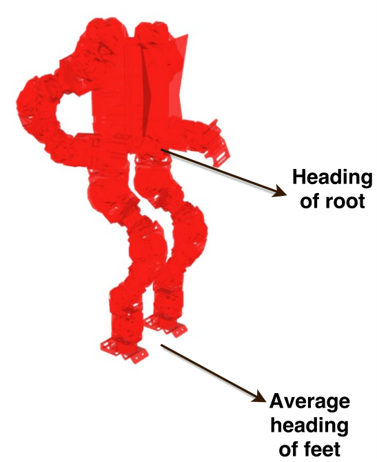
Difference in heading between the root of the robot and the feet of the robot (Fig.4)
- 3.
Euclidean distance between COM of the current state and that of the target state
- 4.
Euclidean distance between active feet of the current state and that of the target state (Fig.4)
- 5.
Curve to provide guidance for stepping feet movement during the search (Fig.4)
- 6.
Remaining number of steps on the lower dimensional path that need to be tracked


VIII Experience Graphs
This section details the method used for accelerating planning when the search must find paths through the high-dimensional space during the second phase of each search iteration. Many of the transitions on the adaptively-dimensional path are directly executable by one of the available controllers, but some transitions require planning in the high-dimensional space. The transitions we focus on in this section are specifically those transitions for the full-body which move between states of different dimensionalities. For example, during the first phase, the planner may produce a transition from the bipedal representation to the ladder representation, which corresponds to the motion for the robot that mounts the ladder while standing in front it.
To speed up high-dimensional planning in these scenarios, we apply Experience Graphs, outlined in [16]. Experience Graphs, or E-Graphs, provide a way to incorporate prior experience, in our case from user demonstrations, to guide the search towards reusing paths with a good chance of leading to the goal. In our domain, these transitions are often similar and we can leverage previous solutions to generate modified transitions quickly.
VIII-A Heuristic Computation
As discussed in [16], the E-Graphs approach defines the heuristic value for a state as
where is a path , , and is a scalar parameter , which determines the degree to which the search is encouraged to reuse prior experience. The paths consist of edges between any two states and with cost equal to the underlying heuristic , inflated by , and edges from the E-Graph with cost equal to the actual cost of the transition.
The underlying heuristic used with the E-Graph heuristic is computed by solving a lower-dimensional problem using dynamic programming. Similar to the heuristics used during the first phase of the search, we solve several 3D Dijkstra searches, each from the goal position of one of the end effectors. The E-Graph transitions, as well as obstacles, are incorporated directly into these Dijkstra expansions to encourage obstacle avoidance and use of prior experience. When computing the heuristic value for a given full-body state, we sum up the contributions from these Dijkstra searches, using the current end effector positions.


VIII-B Snap Motions
In many scenarios, the search can encounter difficulty using the path demonstrations, even if the path is representative of the expected path the robot should take. For example, consider a scenario where a user has demonstrated how the robot should mount a ladder. If, during planning, the search considers a state where the feet are slightly offset from the demonstration, it will still have to reason about the motion required to adjust the feet so that the demonstration can be reused. To alleviate this problem, we combine the ideas from [16] and [17] to create a set of adaptive motion primitives that reach partial states on the E-Graph. For example in the aforementioned scenario, the adaptive motion primitive will attempt to match partial waypoints for the arms and the torso, rather than trying to adjust the feet to match the demonstration completely.
IX Interleaved Planning and Execution
Owing to the complexity of the planning tasks that we are addressing, the typical planning times to plan a path all the way from the start to the goal are significantly high. The key idea here is that instead of waiting for the planner to generate the entire executable path, we will interleave path planning and execution. The planner will return partial plan as it runs while the controller will start executing these plans on the robot in parallel. This idea has been widely studied by the real-time family of heuristic search algorithms. For the humanoid domain this approach provides significant speed ups in the overall planning and execution time because the path execution is generally slow.
Within the underlying framework of planning with adaptive dimensionality, we only employ the interleaving scheme in the tracking phase, because the tracking phase returns a path that is executable by the robot.
X Controller Framework
The path returned by the planner contains both transitions that correspond to executing an available controller, e.g. walking, crawling, climbing, and those that correspond to raw full-body joint motion. As described in Section V, the low-dimensional transitions are directly executable by a controller. It is then the responsibility of the controller to compute full-body joint trajectories that robustly execute the desired motion. Each individual controller only accepts paths of their respective waypoint type. To interface the controllers with the planner, we developed a meta-controller for dispatching segments of the hybrid path to the correct controller. After a hybrid path is received from planner, the meta-controller divides it into the individual segments of the same waypoint type and dispatches them sequentially to the corresponding controllers. After a segment is executed successfully, the controller signals the meta-controller to proceed. The meta-controller then dispatches the next segment to the corresponding controller, until the path is completed. The meta-controller is also responsible for updating the path, as additional waypoints are received during interleaved planning and execution.
XI Experimental Analysis
| success % | mean time (s) | |||
|---|---|---|---|---|
| goal | plan | track | plan | track |
| top | 89.6 | 57.5 | 58.79 | 42.53 |
| mid | 89.6 | 65.7 | 57.67 | 33.61 |
To demonstrate the effectiveness of the multi-heuristic adaptive planning approach, we tested the planner’s ability to plan paths in the sample environment from Figure 1(c). The tests consisted of running the planner from numerous start locations, evenly distributed across (x, y) locations in the environment and from different start headings, to goal locations on the mid- and top-level platforms. In all cases, the planner was given to find a low-dimensional path, and to find the high-dimensional path. The results are shown Table I.
The table lists the results across 231 different start locations, for each goal. Success rates are shown for both the low-dimensional phase of the search, and for the high-dimensional of the search. The success rates for the second ”tracking” phase, are normalized with respect to the success of the first phase, thus the overall success rates for the planner are and , respectively for the two goals.
The columns containing planning times are mean times for the two phases of the search individually. The total average planning times are and seconds, respectively. Note that, outside of experiments, the planning is interleaved with execution of the path on the robot, so the time spent idle is only limited by the time taken by the search during the low- dimensional planning phase, plus a small lookahead for the high-dimensional search. The same is also true for the success rate, where the search is only limited by the speed of execution.
XII Conclusion
In this work, we have presented an approach to planning for multi-modal humanoid mobility using a single search algorithm. This approach is able to simultaneously reason about all the capabilities of the robot, incorporate the capabilities of available controllers, and automatically discover the transitions for switching between modes of locomotion. The resulting planner brings together planning with an adaptively-dimensional search space, using multiple heuristics, and incorporating user demonstrations to concentrate search efforts where they’re most needed. In future work we hope to incorporate planning for more complex interaction with the environment and address the robustness of scenarios requiring high-dimensional planning.
References
- [1] S. J. Yi, S. McGill, L. Vadakedathu, Q. He, I. Ha, J. Han, H. Song, M. Rouleau, D. Hong, and D. D. Lee, “Thor-op humanoid robot for darpa robotics challenge trials 2013,” in 2014 11th International Conference on Ubiquitous Robots and Ambient Intelligence (URAI), Nov 2014, pp. 359–363.
- [2] C. G. Atkeson, B. P. W. Babu, N. Banerjee, D. Berenson, C. P. Bove, X. Cui, M. DeDonato, R. Du, S. Feng, P. Franklin, M. Gennert, J. P. Graff, P. He, A. Jaeger, J. Kim, K. Knoedler, L. Li, C. Liu, X. Long, T. Padir, F. Polido, G. G. Tighe, and X. Xinjilefu, “No falls, no resets: Reliable humanoid behavior in the darpa robotics challenge,” in 2015 IEEE-RAS 15th International Conference on Humanoid Robots (Humanoids), Nov 2015, pp. 623–630.
- [3] Y. Zhang, J. Luo, K. Hauser, H. A. Park, M. Paldhe, C. S. G. Lee, R. Ellenberg, B. Killen, P. Oh, J. H. Oh, J. Lee, and I. Kim, “Motion planning and control of ladder climbing on drc-hubo for darpa robotics challenge,” in 2014 IEEE International Conference on Robotics and Automation (ICRA), May 2014, pp. 2086–2086.
- [4] J. Kuffner, K. Nishiwaki, S. Kagami, M. Inaba, and H. Inoue, “Motion planning for humanoid robots,” Robotics Research, pp. 365–374, 2005.
- [5] A. Hornung, A. Dornbush, M. Likhachev, and M. Bennewitz, “Anytime search-based footstep planning with suboptimality bounds,” in Humanoid Robots (Humanoids), 2012 12th IEEE-RAS International Conference on. IEEE, 2012, pp. 674–679.
- [6] F. Burget, A. Hornung, and M. Bennewitz, “Whole-body motion planning for manipulation of articulated objects,” in 2013 IEEE International Conference on Robotics and Automation, May 2013, pp. 1656–1662.
- [7] A. Athar, A. M. Zafar, R. Asif, A. A. Khan, F. Islam, O. Hasan, et al., “Whole-body motion planning for humanoid robots with heuristic search,” in Intelligent Robots and Systems (IROS), 2016 IEEE/RSJ International Conference on. IEEE, 2016, pp. 4720–4727.
- [8] S. Dalibard, A. Nakhaei, F. Lamiraux, and J. P. Laumond, “Whole-body task planning for a humanoid robot: a way to integrate collision avoidance,” in 2009 9th IEEE-RAS International Conference on Humanoid Robots, Dec 2009, pp. 355–360.
- [9] Y. Zhang, J. Luo, K. Hauser, R. Ellenberg, P. Oh, H. A. Park, M. Paldhe, and C. S. G. Lee, “Motion planning of ladder climbing for humanoid robots,” in 2013 IEEE Conference on Technologies for Practical Robot Applications (TePRA), April 2013, pp. 1–6.
- [10] M. Kanazawa, S. Nozawa, Y. Kakiuchi, Y. Kanemoto, M. Kuroda, K. Okada, M. Inaba, and T. Yoshiike, “Robust vertical ladder climbing and transitioning between ladder and catwalk for humanoid robots,” in 2015 IEEE/RSJ International Conference on Intelligent Robots and Systems (IROS), Sept 2015, pp. 2202–2209.
- [11] N. Vahrenkamp, C. Scheurer, T. Asfour, J. Kuffner, and R. Dillmann, “Adaptive motion planning for humanoid robots,” in 2008 IEEE/RSJ International Conference on Intelligent Robots and Systems, Sept 2008, pp. 2127–2132.
- [12] C. Park, J. Pan, and D. Manocha, “High-dof robots in dynamic environments using incremental trajectory optimization,” International Journal of Humanoid Robotics, vol. 11, no. 02, p. 1441001, 2014.
- [13] K. Gochev, B. Cohen, J. Butzke, A. Safonova, and M. Likhachev, “Path planning with adaptive dimensionality,” in Fourth annual symposium on combinatorial search, 2011.
- [14] K. Gochev, A. Safonova, and M. Likhachev, “Planning with adaptive dimensionality for mobile manipulation,” in Robotics and Automation (ICRA), 2012 IEEE International Conference on. IEEE, 2012, pp. 2944–2951.
- [15] S. Aine, S. Swaminathan, V. Narayanan, V. Hwang, and M. Likhachev, “Multi-heuristic a*,” The International Journal of Robotics Research, vol. 35, no. 1-3, pp. 224–243, 2016.
- [16] M. Phillips, B. J. Cohen, S. Chitta, and M. Likhachev, “E-graphs: Bootstrapping planning with experience graphs.” in Robotics: Science and Systems, vol. 5, no. 1, 2012.
- [17] B. Cohen, G. Subramanian, S. Chitta, and M. Likhachev, “Planning for manipulation with adaptive motion primitives,” in Robotics and Automation (ICRA), 2011 IEEE International Conference on, 2011.