跳到论文正文
W Papers独立论文阅读器 arXiv:1801.10137 论文正文 计算阅读时间 · 0%
引用这篇论文根据当前论文元数据生成,正式投稿前建议核对。


License: arXiv.org perpetual non-exclusive license
arXiv:1801.10137v2 [hep-ph] 17 Jul 2018

Inclusive 𝒉𝒄{\bm{h}}_{\bm{c}} production and energy spectrum from 𝒆+​𝒆−{\bm{e}}^{\bm{+}}{\bm{e}}^{\bm{-}} annihilation at Super 𝑩\bm{B} factory

Qing-Feng Sun Note: qfsun@mail.ustc.edu.cn Affiliation: Department of Modern Physics, University of Science and Technology of China, Hefei, Anhui 230026, China Affiliation: Institute of High Energy Physics, Chinese Academy of Sciences, Beijing 100049, China    Yu Jia Note: jiay@ihep.ac.cn Affiliation: Institute of High Energy Physics, Chinese Academy of Sciences, Beijing 100049, China    Xiaohui Liu Note: xiliu@bnu.edu.cn Affiliation: Center of Advanced Quantum Studies and Department of Physics, Beijing Normal University, Beijing, 100875, China    Ruilin Zhu Note: rlzhu@njnu.edu.cn Affiliation: Department of Physics and Institute of Theoretical Physics, Nanjing Normal University, Nanjing, Jiangsu 210023, China
August 24, 2026
Abstract

We calculate the next-to-leading order (NLO) radiative correction to the color-octet hch_{c} inclusive production in e+​e−e^{+}e^{-} annihilation at Super BB factory, within the nonrelativistic QCD factorization framework. The analytic expression for the NLO short-distance coefficient (SDC) accompanying the color-octet production operator 𝒪8hc(1S0)\mathcal{O}_{8}^{h_{c}}(^{1}S_{0}) is obtained after summing both virtual and real corrections. The size of NLO correction for the color-octet production channel is found to be positive and substantial. The NLO prediction to the hch_{c} energy spectrum is plagued with unphysical endpoint singularity. With the aid of the soft-collinear effective theory, those large endpoint logarithms are resummed to the next-to-leading logarithmic (NLL) accuracy. Consequently, further supplemented with the non-perturbative shape function, we obtain the well-behaved predictions for the hch_{c} energy spectrum in the entire kinematic range, which awaits the examination by the forthcoming Belle II experiment.

pacs
12.38.Bx, 12.38.Cy, 14.40.Pq, 12.39.Hg

I Introduction

The hc​(1​P)h_{c}(1P) meson, the lowest-lying spin-singlet PP-wave charmonium, is the last member found among the charmonium family below the open charm threshold. The first hint about its existence was reported in the process p​p¯→hc→J/ψ​π0p\bar{p}\to h_{c}\to J/\psi\pi^{0} by the Fermilab E760 experiment in 1992 [1]. Finally, in 2005, the hch_{c} state was firmly established through the process p​p¯→hc→ηc​γp\bar{p}\to h_{c}\to\eta_{c}\gamma in the Fermilab E835 experiment [2], as well as through the isospin-violating charmonium transition process ψ(2S)→hc(→ηcγ)+π0\psi(2S)\to h_{c}(\to\eta_{c}\gamma)+\pi^{0} in the CLEO-c experiment [3, 4]. Later this decay chain was confirmed in the BESIII experiment with much greater data sample [5, 6]. To date, the latest measured mass and width of hch_{c} are Mhc=3525.38±0.11M_{h_{c}}=3525.38\pm 0.11 MeV, and Γhc=0.7±0.28±0.22\Gamma_{h_{c}}=0.7\pm 0.28\pm 0.22 MeV, respectively [7]. Two exclusive decay channels, the electric dipole (E​1E1) radiative transition hc→ηc​γh_{c}\to\eta_{c}\gamma, and the OZI-suppressed annihilation decay hc→2​π+​2​π−​π0h_{c}\to 2\pi^{+}2\pi^{-}\pi^{0}, have been measured, with the corresponding branching fractions ℬ⁡(hc→ηc​γ)=(51±6)%{\mathcal{B}}(h_{c}\to\eta_{c}\gamma)=(51\pm 6)\%, and ℬ⁡(hc→2​π+​2​π−​π0)=(2.2−0.7+0.8)%{\mathcal{B}}(h_{c}\to 2\pi^{+}2\pi^{-}\pi^{0})=(2.2^{+0.8}_{-0.7})\%, respectively [7]. It is worth mentioning that, the P11{}^{1}P_{1} counterparts in the bottomonium family, the hb​(1​P,2​P)h_{b}(1P,2P) mesons, have also recently been established via the di-pion transition from the Υ⁡(5​S)\Upsilon(5S) resonance in the Belle experiment [8].

It is interesting to ask whether one can possibly understand various dynamical aspects of the hch_{c} meson from the first principles of QCD. In fact, nonrelativistic QCD (NRQCD) [9], the modern effective field theory to describe the slowly-moving heavy quark-antiquark system, is an appropriate model-independent framework to tackle a multi-scale system exemplified by the charmonium state hch_{c}. Furthermore, the NRQCD factorization approach [10], originally developed by Bodwin, Braaten and Lepage, provides a powerful and systematic language to describe the inclusive quarkonium production and decay processes, which has been fruitfully applied to uncountable charmonium phenomenologies in the past two decades [11].

For the dominant E​1E1 decay process hc→ηc​γh_{c}\to\eta_{c}\gamma, there have been many preceding studies based on the multipole expansion picture in the quark potential models [12]. Moreover, the radiative and relativistic corrections to the inclusive hadronic widths of hc,bh_{c,b} have recently been investigated in the NRQCD factorization framework [13]. On the other hand, the hch_{c} production in various collision environments have also been extensively investigated in recent years. For instance, hch_{c} inclusive production in BB meson decay [14, 15], hch_{c} photoproduction [16], hch_{c} hadroproduction [17, 18, 19], inclusive hch_{c} production from e+​e−e^{+}e^{-} annihilation [20, 21], exclusive hch_{c} production from Z0Z^{0} decay [22], from double charmonium production in e+​e−e^{+}e^{-} annihilation [23], as well as from Υ⁡(n​S)\Upsilon(nS) decay [24].

The hadroproduction rate of hch_{c} is significant at LHC experiment due to the huge partonic luminosity. A recent computation indicates that the gluon-to-hch_{c} fragmentation probability may reach the order 10−610^{-6} [25]. In sharp contrast to J/ψ⁡(ψ′)J/\psi(\psi^{\prime}) hadroproduction [26, 27, 28, 29, 30], unfortunately it is rather challenging to reconstruct the hch_{c} events via the dominant decay channel hc→ηc​γh_{c}\to\eta_{c}\gamma, due to the tremendous background at hadron collision experiments. In contrast, tagging hch_{c} is much more tractable in the e+​e−e^{+}e^{-} machines than in hadron colliders. For example, the exclusive hch_{c} production process e+​e−→hc​π+​π−e^{+}e^{-}\to h_{c}\pi^{+}\pi^{-} at center-of-mass energy s=4.170\sqrt{s}=4.170 GeV has been studied by the CLEO Collaboration, with the cross section measured to be 15.6±2.3±1.9±3.015.6\pm 2.3\pm 1.9\pm 3.0 pb [31]. They also found evidence for the process e++e−→hc​ηe^{+}+e^{-}\to h_{c}\eta at 3​σ3\sigma confidence level. As a byproduct of studying this exclusive hch_{c} production channel, BESIII have recently found two charmonium-like resonances, namely the Y⁡(4220)Y(4220) and Y⁡(4390)Y(4390) [32].

The forthcoming Belle II experiment (also referred to as Super BB factory) will accumulate a tremendous dataset near the Υ⁡(4​S)\Upsilon(4S) energy. In this paper, we will focus on the inclusive hch_{c} production in e+​e−e^{+}e^{-} annihilation at s≈10.58\sqrt{s}\approx 10.58 GeV, near the Υ⁡(4​S)\Upsilon(4S) resonance. In the previous work [20, 21], the NRQCD SDCs were evaluated for both color-singlet and color-octet channels at the leading order (LO) in αs\alpha_{s}, and it was found that the latter octet-channel production cross section dominated the singlet-channel cross section. Therefore, in order to make a more precise prediction, it is helpful to evaluate the NLO QCD correction to the color-octet cross section. Moreover, to expedite the experimental search for hch_{c}, it is crucial to predict not only the total hch_{c} production rate, but also the differential hch_{c} energy spectrum.

The LO color-octet contribution to the hch_{c} energy spectrum in e+​e−→hc+Xe^{+}e^{-}\to h_{c}+X is simply a δ\delta-function, determined by the partonic process e+​e−→c​c¯​(S(8)01)+ge^{+}e^{-}\to c\bar{c}({}^{1}S_{0}^{(8)})+g. After including the real correction in the color-octet channel, e+​e−→c​c¯​(S(8)01)+g​ge^{+}e^{-}\to c\bar{c}({}^{1}S_{0}^{(8)})+gg, the energy spectrum then becomes continuous over all allowed domain, however turns out to be singular near the upper endpoint, due to the soft and collinear gluon radiation in this limited region of phase space. This signals a breakdown of the fixed-order QCD prediction, and failure of NRQCD expansion near this kinematic endpoint region. The aim of this work is thus two fold. First we extend the LO color-octet NRQCD SDC obtained in [20] to NLO in αs\alpha_{s}, in a fully analytical manner. Secondly, we follow the recipe of the resumming large logarithms in the color-octet channel for the process e+​e−→J/ψ+Xe^{+}e^{-}\to J/\psi+X near the endpoint region [33], which was formulated in the context of the soft-collinear effective theory (SCET) [34, 35, 36, 37, 38, 39], to tame the endpoint singularity encountered in our case, and finally predict a well-behaved hch_{c} energy spectrum. We hope our prediction will provide some useful guidance for unambiguously erecting the hch_{c} state in the forthcoming Belle II experiment.

The rest of the paper is distributed as follows. In Sec. II, the fixed-order calculations for the SDCs are presented within the NRQCD factorization framework. We first review the existing LO results for both color-singlet and octet channels. In Sec. III, we present the analytical expressions for NLO NRQCD SDCs from the color-octet channel, including both virtual and real corrections. In Sec. IV, within the SCET framework, we show how to resum the large endpoint logarithms to the NLL accuracy. In Sec. V, we present our numerical results for the total hch_{c} production rate and its differential energy spectrum. We also discuss the observational prospects of the hc​(1​P,2​P)h_{c}(1P,2P) states in the forthcoming Belle II experiment. Finally we summarize in Sec. VI. In the Appendix, we expound how to analytically carry out the three-body phase space to isolate the soft and collinear divergences in d=4−2​ϵd=4-2\epsilon spacetime dimensions.

II NRQCD factorization and LO Short-distance coefficients

II.1 NRQCD factorization for hch_{c} production

Heavy quarkonium is a QCD bound state predominantly composed of a pair of nonrelativistic heavy quark and antiquark. For the charmonium, the typical velocity between the charm quarks inside a charmonium is roughly v2≈0.3v^{2}\approx 0.3, thus velocity expansion is not anticipated to converge very well. According to the NRQCD factorization theorem [10], the inclusive production rate of hch_{c} can be expressed as a sum of the product of perturbatively calculable NRQCD SDCs and the non-perturbative NRQCD long-distance matrix elements (LDMEs). The importance of the LDMEs is weighed by the power counting in vv. At the lowest order in vv, the differential cross section for inclusive hch_{c} production can be written as [10]

dσ[e+e−→hc+X]=d​F1​(μΛ)mc4⟨𝒪1hc(1P1)⟩+d​F8mc2⟨𝒪8hc(1S0)(μΛ)⟩+⋯,d\sigma[e^{+}e^{-}\to h_{c}+X]=\frac{dF_{1}(\mu_{\Lambda})}{m_{c}^{4}}\langle\mathcal{O}_{1}^{h_{c}}(^{1}P_{1})\rangle+\frac{dF_{8}}{m_{c}^{2}}\langle\mathcal{O}_{8}^{h_{c}}(^{1}S_{0})(\mu_{\Lambda})\rangle+\cdots, (1)

where the SDCs d​F1dF_{1} and d​F8dF_{8} can be calculated order by order in αs\alpha_{s}, ⟨𝒪1hc(1P1)⟩\langle\mathcal{O}_{1}^{h_{c}}(^{1}P_{1})\rangle and ⟨𝒪8hc(1S0)⟩\langle\mathcal{O}_{8}^{h_{c}}(^{1}S_{0})\rangle are the color-singlet and color-octet NRQCD production LDMEs, respectively. The corresponding hch_{c} production operators in NRQCD are defined as [10] 11 1 It was first made clear by Nayak, Qiu and Sterman [40, 41] a decade ago that the original definition of the NRQCD color-octet production operator [10] is not gauge invariant, and the correct definition necessitates the inclusion of eikonal lines that run from the location of the quark/antiquark fields to infinity. To the perturbative order considered in this work, this nuisance does not play a role so we adhere to the conventional definition [10].

𝒪1hc(1P1)=\displaystyle\mathcal{O}_{1}^{h_{c}}(^{1}P_{1})= χ†​(−i2​𝐃⃡)​ψ​∑X|hc+X⟩⋅⟨hc+X|​ψ†​(−i2​𝐃⃡)​χ,\displaystyle\chi^{\dagger}\left(-\frac{i}{2}\tensor{\bf{D}}\right)\psi\sum_{X}|h_{c}+X\rangle\cdot\langle h_{c}+X|\psi^{\dagger}\left(-\frac{i}{2}\tensor{\bf{D}}\right)\chi, (2a)
𝒪8hc(1S0)=\displaystyle\mathcal{O}_{8}^{h_{c}}(^{1}S_{0})= χ†​Ta​ψ​∑X|hc+X⟩⋅⟨hc+X|​ψ†​Ta​χ,\displaystyle\chi^{\dagger}T^{a}\psi\sum_{X}|h_{c}+X\rangle\cdot\langle h_{c}+X|\;\psi^{\dagger}T^{a}\chi, (2b)

where ψ\psi and χ\chi denote the Pauli spinor fields that annihilates a heavy quark and creates a heavy antiquark, respectively. 𝐃⃡\tensor{\bf{D}} represents the left-right symmetric spatial component of the covariant derivative Dμ=∂μ−igsTaAμaD_{\mu}=\partial_{\mu}-ig_{s}T^{a}A_{\mu}^{a}, and TaT^{a} (a=1,…,8a=1,\ldots,8) signifies the generator in the fundamental representation of the S​U​(3)cSU(3)_{c} group. The μΛ\mu_{\Lambda} refers to the NRQCD factorization scale, which lies in the range mc​v≤μΛ≤mcm_{c}v\leq\mu_{\Lambda}\leq m_{c}. These two NRQCD production operators are interconnected through the NRQCD renormalization group equation (RGE) [10]:

dd​ln⁡μΛ2⟨𝒪8hc(1S0)(μΛ)⟩=2​CF​αs​(μΛ)3​π​Nc​mc2⟨𝒪1hc(1P1)⟩.\frac{d}{d\ln\mu^{2}_{\Lambda}}\langle{\cal O}_{8}^{h_{c}}(^{1}S_{0})(\mu_{\Lambda})\rangle=\frac{2C_{F}\alpha_{s}(\mu_{\Lambda})}{3\pi N_{c}m_{c}^{2}}\langle{\cal O}_{1}^{h_{c}}(^{1}P_{1})\rangle. (3)

Being infrared-finite, d​F1dF_{1} and d​F8dF_{8} are insensitive to the long-distance hadronization effects, thus can be determined through the standard perturbative matching procedure. One can replace the physical hch_{c} state in Eq. (1) by the free on-shell c​c¯c\bar{c} pairs with quantum numbers S(8)01{}^{1}S_{0}^{(8)} or P(1)11{}^{1}P_{1}^{(1)}, computing both sides of Eq. (1), demanding both perturbative QCD and perturbative NRQCD to generate identical results. Ultimately, one can solve these two linear equations to ascertain the two SDCs, order by order in αs\alpha_{s}. Here we stress that it is crucial to include the color-octet contribution, otherwise the uncancelled IR divergences emerging from the color-singlet channel would impede the predictive power of NRQCD. For the computation in the QCD side, it is convenient to employ the covariant projection technique [42, 43] to project the c​c¯c\bar{c} amplitude onto the intended LJ2​S+1{}^{2S+1}L_{J} states. Throughout this work, Dimensional Regularization (DR), that is, to work in the spacetime dimensions d=4−2​ϵd=4-2\epsilon, is adopted to regularize both UV and IR divergences.

A kinematical simplification also arises from the ss-channel nature of this process. As long as we are concerned only with the hch_{c} energy distribution, one can reexpress the hch_{c} production rate from e+​e−e^{+}e^{-} annihilation in terms of that from virtual photon decay [44]:

dσ[e+e−→hc+X]=4​π​αs3/2dΓ[γ∗→hc+X],d\sigma\left[e^{+}e^{-}\to h_{c}+X\right]=\frac{4\pi\alpha}{s^{3/2}}d\Gamma\left[\gamma^{*}\to h_{c}+X\right], (4)

where the center-of-mass energy of the e+​e−e^{+}e^{-} system is denoted by s\sqrt{s}.

Refer to caption
Figure 1: Representative Feynman diagrams for the c​c¯​(n)c\bar{c}(n) production from e+​e−e^{+}e^{-} annihilation, for n=S(8)01n={}^{1}S_{0}^{(8)} or P(1)11{}^{1}P_{1}^{(1)}.

Some representative Feynman diagrams for c​c¯​(n)c\bar{c}(n) (n=S(8)01n={}^{1}S_{0}^{(8)} or P(1)11{}^{1}P_{1}^{(1)}) production from e+​e−e^{+}e^{-} annihilation in both color-singlet and color-octet channels are shown in Fig. 1. Due to the odd CC parity of the hch_{c} meson, the color-singlet channel starts at 𝒪⁡(αs2)\mathcal{O}(\alpha^{2}_{s}), while the octet contribution starts at 𝒪⁡(αs)\mathcal{O}(\alpha_{s}). In the rest of this section, we will briefly review the LO results for F8F_{8} and F1F_{1}, which were first analytically evaluated in Ref. [20].

II.2 LO color-octet SDC

At LO in color-octet channel, we only need consider e+​e−→γ∗→c​c¯​(S(8)01)+ge^{+}e^{-}\to\gamma^{*}\to c\bar{c}({}^{1}S_{0}^{(8)})+g. The differential two-body phase space in d=4−2​ϵd=4-2\epsilon dimensions reads [20]

d​Φ2=cϵ8​π​s−ϵ​(1−r)1−2​ϵ​δ​(1+r−z)​d​z,d\Phi_{2}=\frac{c_{\epsilon}}{8\pi}s^{-\epsilon}(1-r)^{1-2\epsilon}\delta(1+r-z)\,dz, (5)

where

cϵ≡(4​π)ϵ​Γ⁡(1−ϵ)Γ⁡(2−2​ϵ),r≡4​mc2s,z≡2​P0s,c_{\epsilon}\equiv(4\pi)^{\epsilon}\frac{\Gamma(1-\epsilon)}{\Gamma(2-2\epsilon)},\qquad r\equiv{4m_{c}^{2}\over s},\qquad z\equiv{2P^{0}\over\sqrt{s}}, (6)

with Pμ=(P0,𝐏)P^{\mu}=(P^{0},\bf{P}) representing the four-momentum of the c​c¯c\bar{c} pair.

The LO amplitude squared turns to be

∑Pol,Col|ℳ(0)[γ∗→cc¯(S01​(8))+g]|2=256π2ec2αCACFαsμr2​ϵ(1−ϵ)(1−2ϵ),\displaystyle\sum_{\text{Pol,Col}}{\left|\mathcal{M}^{(0)}\left[\gamma^{*}\to c\bar{c}(\mathchoice{{\hskip 3.98613pt\hbox{$\displaystyle{S}$}^{\scriptstyle\hskip-3.98613pt\hskip-6.70831pt1\hskip 6.70831pt(8)}_{\scriptstyle\hskip 0.0pt\hskip-6.70831pt\hskip 6.70831pt0}}}{{\hskip 3.98613pt\hbox{$\textstyle{S}$}^{\scriptstyle\hskip-3.98613pt\hskip-6.70831pt1\hskip 6.70831pt(8)}_{\scriptstyle\hskip 0.0pt\hskip-6.70831pt\hskip 6.70831pt0}}}{{\hskip 3.40283pt\hbox{$\scriptstyle{S}$}^{\scriptscriptstyle\hskip-3.40283pt\hskip-5.29308pt1\hskip 5.29308pt(8)}_{\scriptscriptstyle\hskip 0.0pt\hskip-5.29308pt\hskip 5.29308pt0}}}{{\hskip 3.40283pt\hbox{$\scriptscriptstyle{S}$}^{\scriptscriptstyle\hskip-3.40283pt\hskip-4.53476pt1\hskip 4.53476pt(8)}_{\scriptscriptstyle\hskip 0.0pt\hskip-4.53476pt\hskip 4.53476pt0}}})+g\right]\right|^{2}}=256\pi^{2}e_{c}^{2}\alpha C_{A}C_{F}\alpha_{s}\mu_{r}^{2\epsilon}(1-\epsilon)(1-2\epsilon), (7)

where ec=23e_{c}=\frac{2}{3} is the electric charge of the charm quark, CA=3C_{A}=3 and CF=43C_{F}={4\over 3} are the Casimirs of the color S​U​(3)cSU(3)_{c} group. Integrating Eq. (7) over the two-body phase space in Eq. (5), we obtain

σ^LO(8)≡\displaystyle\hat{\sigma}_{\text{LO}}^{(8)}\equiv 2​π​α3​s2∫dΦ2∑Pol,Col|ℳ(0)[γ∗→cc¯(S01​(8))+g]|2\displaystyle\frac{2\pi\alpha}{3s^{2}}\int{d\Phi_{2}}\,\sum_{\text{Pol,Col}}{\left|\mathcal{M}^{(0)}\left[\gamma^{*}\to c\bar{c}(\mathchoice{{\hskip 3.98613pt\hbox{$\displaystyle{S}$}^{\scriptstyle\hskip-3.98613pt\hskip-6.70831pt1\hskip 6.70831pt(8)}_{\scriptstyle\hskip 0.0pt\hskip-6.70831pt\hskip 6.70831pt0}}}{{\hskip 3.98613pt\hbox{$\textstyle{S}$}^{\scriptstyle\hskip-3.98613pt\hskip-6.70831pt1\hskip 6.70831pt(8)}_{\scriptstyle\hskip 0.0pt\hskip-6.70831pt\hskip 6.70831pt0}}}{{\hskip 3.40283pt\hbox{$\scriptstyle{S}$}^{\scriptscriptstyle\hskip-3.40283pt\hskip-5.29308pt1\hskip 5.29308pt(8)}_{\scriptscriptstyle\hskip 0.0pt\hskip-5.29308pt\hskip 5.29308pt0}}}{{\hskip 3.40283pt\hbox{$\scriptscriptstyle{S}$}^{\scriptscriptstyle\hskip-3.40283pt\hskip-4.53476pt1\hskip 4.53476pt(8)}_{\scriptscriptstyle\hskip 0.0pt\hskip-4.53476pt\hskip 4.53476pt0}}})+g\right]\right|^{2}}
=\displaystyle= (4​π​μr2s)ϵ​Γ⁡(2−ϵ)Γ⁡(1−2​ϵ)​64​π2​ec2​α2​CA​CF​αs​(1−r)1−2​ϵ3​s2.\displaystyle\left(\frac{4\pi\mu_{r}^{2}}{s}\right)^{\epsilon}\frac{\Gamma(2-\epsilon)}{\Gamma(1-2\epsilon)}\frac{64\pi^{2}e_{c}^{2}\alpha^{2}C_{A}C_{F}\alpha_{s}(1-r)^{1-2\epsilon}}{3s^{2}}. (8)

The factor 13\frac{1}{3} accounts for averaging over the three polarizations of γ∗\gamma^{*}. The differential expression of σ^LO(8)\hat{\sigma}_{\text{LO}}^{(8)} in 44 dimensions reads

d​σ^LO(8)d​z|d→4=64​π2​ec2​α2​CA​CF​αs​(1−r)3​s2​δ​(1+r−z).\left.\frac{d\hat{\sigma}_{\text{LO}}^{(8)}}{dz}\right|_{d\to 4}=\frac{64\pi^{2}e_{c}^{2}\alpha^{2}C_{A}C_{F}\alpha_{s}(1-r)}{3s^{2}}\delta(1+r-z). (9)

Substituting Eq. (9) to the left hand side of Eq. (1), and only retaining the NRQCD matrix element in the color-octet channel, we then deduce the LO color-octet SDC:

d​F8LOd​z=mc⟨𝒪8c​c¯​(S01)⟩​d​σ^LO(8)d​z=64​π2​ec2​α2​CA​CF​αs​(1−r)​mc3​(Nc2−1)​s2​δ​(1+r−z),{dF_{8}^{\rm LO}\over dz}={m_{c}\over\langle\mathcal{O}_{8}^{c\bar{c}}({}^{1}S_{0})\rangle}{d\hat{\sigma}_{\text{LO}}^{(8)}\over dz}={64\pi^{2}e_{c}^{2}\alpha^{2}C_{A}C_{F}\alpha_{s}(1-r)m_{c}\over 3(N_{c}^{2}-1)s^{2}}\delta(1+r-z), (10)

where we have used ⟨𝒪8c​c¯​(S01)⟩=Nc2−1\langle\mathcal{O}_{8}^{c\bar{c}}({}^{1}S_{0})\rangle=N_{c}^{2}-1. The integrated color-octet SDC is then

F8LO=64​π2​ec2​α2​CA​CF​αs​(1−r)​mc3​(Nc2−1)​s2,F_{8}^{\rm LO}={64\pi^{2}e_{c}^{2}\alpha^{2}C_{A}C_{F}\alpha_{s}(1-r)m_{c}\over 3(N_{c}^{2}-1)s^{2}}, (11)

which scales as 1/s21/s^{2} asymptotically.

II.3 LO color-singlet SDC

To determine the LO SDC in the color-singlet channel, we need consider the partonic process e+​e−→c​c¯​(P(1)11)+g​ge^{+}e^{-}\to c\bar{c}({}^{1}P_{1}^{(1)})+gg. The IR divergence appears in the upper endpoint of the hch_{c} spectrum, when one of the gluons becomes soft. It is most convenient to handle this IR singularity using DR. As a virtue of the color-octet mechanism of NRQCD, the single IR pole is factored into the color-octet NRQCD LDME. As a remnant of this IR divergence, the renormalized color-octet LDME is defined at the NRQCD factorization scale μΛ\mu_{\Lambda}, in the meanwhile the SDC F1F_{1} acquires an explicit logarithmic dependence on μΛ\mu_{\Lambda}. The differential color-singlet SDC d​F1/d​zdF_{1}/dz is somewhat too lengthy to reproduce here, and we refer the interested readers to Ref. [20] for its complete expression. Here we just present the integrated color-singlet SDC:

F1LO​(μΛ)=\displaystyle F_{1}^{\text{LO}}(\mu_{\Lambda})= 64​π​ec2​α2​CF​αs2​mc9​Nc​s2(1−r)[−lnμΛ24​mc2+2ln(1−r)−65−84​r12​(1−r)+7+7​r−9​r26​(1−r)2lnr\displaystyle\frac{64\pi e_{c}^{2}\alpha^{2}C_{F}\alpha_{s}^{2}m_{c}}{9N_{c}s^{2}}(1-r)\left[-\ln{\frac{\mu_{\Lambda}^{2}}{4m_{c}^{2}}}+2\ln{(1-r)}-\frac{65-84r}{12(1-r)}+\frac{7+7r-9r^{2}}{6(1-r)^{2}}\ln{r}\right.
+r⁡(5−7​r)16​(1−r)2ln21+1−r1−1−r+14−15​r8​(1−r)3/2ln1+1−r1−1−r],\displaystyle\left.+\frac{r(5-7r)}{16(1-r)^{2}}\ln^{2}{\frac{1+\sqrt{1-r}}{1-\sqrt{1-r}}}+\frac{14-15r}{8(1-r)^{3/2}}\ln{\frac{1+\sqrt{1-r}}{1-\sqrt{1-r}}}\right], (12)

which is obtained according to the MS¯\overline{\rm MS} renormalization scheme. It is enlightening to see the asymptotic behavior of F1LOF_{1}^{\text{LO}} in the s≫mc\sqrt{s}\gg m_{c} limit:

F1LO​(μΛ)|Asym.=64​π​ec2​α2​CF​αs2​mc9​Nc​s2​(−712​ln⁡r−ln⁡μΛ24​mc2−6512+72​ln⁡2),F_{1}^{\text{LO}}(\mu_{\Lambda})\Big|_{\rm Asym.}=\frac{64\pi e_{c}^{2}\alpha^{2}C_{F}\alpha_{s}^{2}m_{c}}{9N_{c}s^{2}}\left(-\frac{7}{12}\ln{r}-\ln{\frac{\mu_{\Lambda}^{2}}{4m_{c}^{2}}}-\frac{65}{12}+\frac{7}{2}\ln{2}\right), (13)

which is proportional to 1/s21/s^{2} times a single logarithm of s/mc2s/m_{c}^{2}.

III NLO radiative correction for the color-octet channel

In this section, we are going to calculate the NLO radiative correction for the color-octet SDC d​F8dF_{8}, which includes the real correction e+​e−→c​c¯​(S(8)01)+g​g​(q​q¯)e^{+}e^{-}\to c\bar{c}({}^{1}S_{0}^{(8)})+gg(q\bar{q}), together with the one-loop virtual correction to e+​e−→c​c¯​(S(8)01)+ge^{+}e^{-}\to c\bar{c}({}^{1}S_{0}^{(8)})+g. The UV divergences encountered in virtual correction will be eliminated by the standard renormalization procedure, while the IR singularities turn out to cancel out after summing both real and virtual corrections.

In the NLO calculation, we generate the QCD Feynman diagrams and amplitudes using the package FeynArts [45], and employ the package FeynCalc [46] to carry out contraction of the Lorentz indices and trace over Dirac matrices. We use the Feynman gauge throughout the calculation.

III.1 Real correction

There are more Feyman diagrams for e+​e−→γ∗→c​c¯​(S(8)01)+g​ge^{+}e^{-}\to\gamma^{*}\to c\bar{c}({}^{1}S_{0}^{(8)})+gg than the color-singlet channel, since the three-gluon vertex is permitted due to the color-octet feature of the c​c¯c\bar{c} pair. Furthermore, the new channel e+​e−→γ∗→c​c¯​(S(8)01)+q​q¯e^{+}e^{-}\to\gamma^{*}\to c\bar{c}({}^{1}S_{0}^{(8)})+q\bar{q} also becomes permissible. One typical real emission diagram is depicted in Fig. 1.

In this section, we will quickly present the analytic results by integrating the squared amplitudes over the three-body phase space in DR, closely following the recipe outlined in Ref. [20]. To ensure the correctness of our results, we also redo the calculation using numerical recipe, i.e., utilizing the two-cutoff phase space slicing method [47], and find full agreement with our analytical results.

First, let us introduce, in addition to zz, two additional fractional energy variables, x1x_{1} and x2x_{2}:

x1≡2​k10s,x2≡2​k20s,x_{1}\equiv\frac{2k_{1}^{0}}{\sqrt{s}},\qquad x_{2}\equiv\frac{2k_{2}^{0}}{\sqrt{s}}, (14)

where k1k_{1} and k2k_{2} represent the momenta of the final-state gluons (or light quark and antiquark) in real emission process. These variables are subject to the constraint x1+x2+z=2x_{1}+x_{2}+z=2 by energy conservation.

For convenience, we separate the squared amplitude for γ∗→c​c¯​(S01​(8))+g​g\gamma^{*}\to c\bar{c}(\mathchoice{{\hskip 3.98613pt\hbox{$\displaystyle{S}$}^{\scriptstyle\hskip-3.98613pt\hskip-6.70831pt1\hskip 6.70831pt(8)}_{\scriptstyle\hskip 0.0pt\hskip-6.70831pt\hskip 6.70831pt0}}}{{\hskip 3.98613pt\hbox{$\textstyle{S}$}^{\scriptstyle\hskip-3.98613pt\hskip-6.70831pt1\hskip 6.70831pt(8)}_{\scriptstyle\hskip 0.0pt\hskip-6.70831pt\hskip 6.70831pt0}}}{{\hskip 3.40283pt\hbox{$\scriptstyle{S}$}^{\scriptscriptstyle\hskip-3.40283pt\hskip-5.29308pt1\hskip 5.29308pt(8)}_{\scriptscriptstyle\hskip 0.0pt\hskip-5.29308pt\hskip 5.29308pt0}}}{{\hskip 3.40283pt\hbox{$\scriptscriptstyle{S}$}^{\scriptscriptstyle\hskip-3.40283pt\hskip-4.53476pt1\hskip 4.53476pt(8)}_{\scriptscriptstyle\hskip 0.0pt\hskip-4.53476pt\hskip 4.53476pt0}}})+gg into four pieces:

∑Pol,Col|ℳR[γ∗→cc¯(S01​(8))+gg]|2=ℐS(xi,z)+ℐC(xi,z)+ℐSC(xi,z)+ℐFin(xi,z),\sum_{\text{Pol,Col}}{\left|{\mathcal{M}}^{\rm R}\left[\gamma^{*}\to c\bar{c}(\mathchoice{{\hskip 3.98613pt\hbox{$\displaystyle{S}$}^{\scriptstyle\hskip-3.98613pt\hskip-6.70831pt1\hskip 6.70831pt(8)}_{\scriptstyle\hskip 0.0pt\hskip-6.70831pt\hskip 6.70831pt0}}}{{\hskip 3.98613pt\hbox{$\textstyle{S}$}^{\scriptstyle\hskip-3.98613pt\hskip-6.70831pt1\hskip 6.70831pt(8)}_{\scriptstyle\hskip 0.0pt\hskip-6.70831pt\hskip 6.70831pt0}}}{{\hskip 3.40283pt\hbox{$\scriptstyle{S}$}^{\scriptscriptstyle\hskip-3.40283pt\hskip-5.29308pt1\hskip 5.29308pt(8)}_{\scriptscriptstyle\hskip 0.0pt\hskip-5.29308pt\hskip 5.29308pt0}}}{{\hskip 3.40283pt\hbox{$\scriptscriptstyle{S}$}^{\scriptscriptstyle\hskip-3.40283pt\hskip-4.53476pt1\hskip 4.53476pt(8)}_{\scriptscriptstyle\hskip 0.0pt\hskip-4.53476pt\hskip 4.53476pt0}}})+gg\right]\right|^{2}}=\mathcal{I}_{\text{S}}(x_{i},z)+\mathcal{I}_{\text{C}}(x_{i},z)+\mathcal{I}_{\text{SC}}(x_{i},z)+\mathcal{I}_{\text{Fin}}(x_{i},z), (15)

with i=1,2i=1,2. Explicitly, these four pieces are

ℐS​(xi,z)=\displaystyle\mathcal{I}_{\text{S}}(x_{i},z)= −212​π3​ec2​α​CA2​CF​αs2​μr4​ϵ​(1−ϵ)​(1−2​ϵ)​rs​[1(1+r−z−x1)2+1(1+r−z−x2)2],\displaystyle-\frac{2^{12}\pi^{3}e_{c}^{2}\alpha C_{A}^{2}C_{F}\alpha_{s}^{2}\mu_{r}^{4\epsilon}\left(1-\epsilon\right)\left(1-2\epsilon\right)r}{s}\left[\frac{1}{\left(1+r-z-x_{1}\right)^{2}}+\frac{1}{\left(1+r-z-x_{2}\right)^{2}}\right], (16a)
ℐC​(xi,z)=\displaystyle{\cal I}_{\rm C}(x_{i},z)= 212​π3​ec2​α​CA2​CF​αs2​μr4​ϵ​(1−ϵ)​(1−2​ϵ)(1−r)2​s​x1​x2−2​(1−r)21+r−z,\displaystyle{2^{12}\pi^{3}e_{c}^{2}\alpha C_{A}^{2}C_{F}\alpha_{s}^{2}\mu_{r}^{4\epsilon}(1-\epsilon)(1-2\epsilon)\over(1-r)^{2}s}{x_{1}x_{2}-2(1-r)^{2}\over 1+r-z}, (16b)
ℐSC​(xi,z)=\displaystyle\mathcal{I}_{\text{SC}}(x_{i},z)= −212​π3​ec2​α​CA2​CF​αs2​μr4​ϵ​(1−ϵ)​(1−2​ϵ)​(1−r)s​11+r−z​(11+r−z−x1+11+r−z−x2),\displaystyle-\frac{2^{12}\pi^{3}e_{c}^{2}\alpha C_{A}^{2}C_{F}\alpha_{s}^{2}\mu_{r}^{4\epsilon}\left(1-\epsilon\right)\left(1-2\epsilon\right)(1-r)}{s}\frac{1}{1+r-z}\left(\frac{1}{1+r-z-x_{1}}+\frac{1}{1+r-z-x_{2}}\right), (16c)
ℐFin​(xi,z)=\displaystyle{\cal I}_{\rm Fin}(x_{i},z)= 212​π3​ec2​α​CA2​CF​αs2(1−r)2​(2−z)2​(1−r−x1)2​(1−r−x2)2​s{(1−r)3(1+r−z)(z−2r)(2−z)2\displaystyle{2^{12}\pi^{3}e_{c}^{2}\alpha C_{A}^{2}C_{F}\alpha_{s}^{2}\over(1-r)^{2}(2-z)^{2}(1-r-x_{1})^{2}(1-r-x_{2})^{2}s}\bigg\{(1-r)^{3}(1+r-z)(z-2r)(2-z)^{2}
−(1−r)3(5+2r+r2−5z−rz+z2)x1x2+2(1−r)(2−z)2x12x22−(3−r−z)x13x23}.\displaystyle-(1-r)^{3}(5+2r+r^{2}-5z-rz+z^{2})x_{1}x_{2}+2(1-r)(2-z)^{2}x_{1}^{2}x_{2}^{2}-(3-r-z)x_{1}^{3}x_{2}^{3}\bigg\}. (16d)

Each individual term is symmetric under the exchange x1↔x2x_{1}\leftrightarrow x_{2}, reflecting the Bose symmetry of the two gluons in the final state. Upon phase space integration, the first term ℐS\mathcal{I}_{\text{S}} would lead to a single soft pole, when one of the gluons becomes soft. The second term ℐC\mathcal{I}_{\text{C}} would result in a single collinear pole, when the final-state gluons become collinear to each other. The third term ℐSC\mathcal{I}_{\text{SC}} would produce the double IR pole, arising from the corner of phase space where one of the gluons becomes simultaneously soft and collinear to the other one. Note both soft and collinear singularities can arise only when the c​c¯c\bar{c} pair acquires its maximal energy, that is, in the z→1+rz\to 1+r limit. The last term ℐFin\mathcal{I}_{\text{Fin}} will not result in any IR divergences upon phase space integration, therefore can be directly treated in 4 spacetime dimensions.

Integrating the squared amplitudes in Eq. (15) over the three-body phase space, we obtain

σ^R(8),g​g≡σ^Div(8),g​g+σ^Fin(8),g​g,\hat{\sigma}_{\text{R}}^{(8),gg}\equiv\hat{\sigma}_{\text{Div}}^{(8),gg}+\hat{\sigma}_{\text{Fin}}^{(8),gg}, (17)

where the “divergent” and “finite” partonic cross sections are defined as

σ^Div(8),g​g=\displaystyle\hat{\sigma}_{\text{Div}}^{(8),gg}= ∫2​r1+rd​z​d​σ^Div(8),g​gd​z=12!​2​π​α3​s2​∫d​Φ3​[ℐS​(xi,z)+ℐC​(xi,z)+ℐSC​(xi,z)],\displaystyle\int_{2\sqrt{r}}^{1+r}dz\frac{d\hat{\sigma}_{\text{Div}}^{(8),gg}}{dz}=\frac{1}{2!}\frac{2\pi\alpha}{3s^{2}}\int{d\Phi_{3}}\,\left[\mathcal{I}_{\text{S}}\left(x_{i},z\right)+\mathcal{I}_{\text{C}}(x_{i},z)+\mathcal{I}_{\text{SC}}(x_{i},z)\right], (18a)
σ^Fin(8),g​g=\displaystyle\hat{\sigma}_{\text{Fin}}^{(8),gg}= ∫2​r1+rd​z​d​σ^Fin(8),g​gd​z=12!​2​π​α3​s2​∫d​Φ3​ℐFin​(xi,z).\displaystyle\int_{2\sqrt{r}}^{1+r}dz\frac{d\hat{\sigma}_{\text{Fin}}^{(8),gg}}{dz}=\frac{1}{2!}\frac{2\pi\alpha}{3s^{2}}\int{d\Phi_{3}}\,\mathcal{I}_{\text{Fin}}\left(x_{i},z\right). (18b)

Here d​Φ3d\Phi_{3} signifies the three-body phase space measure, whose exact definition in d=4−2​ϵd=4-2\epsilon dimensions is given in Eq. (A.1). We have also included a symmetry factor 12!{1\over 2!} in Eq. (18), to account for the indistinguishability of the final-state gluons.

By carrying out one-fold integration over x1x_{1} in Eq. (18), we then arrive at the partonic cross section differential in the energy fraction of the c​c¯c\bar{c} pair:

d​σ^Div(8),g​gd​z=\displaystyle\frac{d\hat{\sigma}_{\text{Div}}^{(8),gg}}{dz}= σ^LO(8)​αsπ​(1−r)−2​ϵ​rϵΓ⁡(1−ϵ)​(4​π​μr2s)ϵ\displaystyle\hat{\sigma}_{\text{LO}}^{(8)}\frac{\alpha_{s}}{\pi}\frac{(1-r)^{-2\epsilon}r^{\epsilon}}{\Gamma\left(1-\epsilon\right)}\left(\frac{4\pi\mu_{r}^{2}}{s}\right)^{\epsilon}
×CA{(12​ϵ2+17121ϵ−2ln2r1+r−236lnr1+r−π24+6736)δ(1+r−z)\displaystyle\times C_{A}\Bigg\{\left(\frac{1}{2\epsilon^{2}}+\frac{17}{12}\frac{1}{\epsilon}-2\ln^{2}{\frac{\sqrt{r}}{1+\sqrt{r}}}-\frac{23}{6}\ln{\frac{\sqrt{r}}{1+\sqrt{r}}}-\frac{\pi^{2}}{4}+\frac{67}{36}\right)\delta(1+r-z)
+[11+r−z]+[2ln2−z+z2−4​r2−lnz−z2−4​rz+z2−4​r\displaystyle+\left[\frac{1}{1+r-z}\right]_{+}\left[2\ln{\frac{2-z+\sqrt{z^{2}-4r}}{2}}-\ln{\frac{z-\sqrt{z^{2}-4r}}{z+\sqrt{z^{2}-4r}}}\right.
−2​z2−4​r1−r+z2−4​r​(6+2​r−6​z+z2)12​(1−r)3]−[ln⁡(1+r−z)1+r−z]+},\displaystyle\left.-\frac{2\sqrt{z^{2}-4r}}{1-r}+\frac{\sqrt{z^{2}-4r}\left(6+2r-6z+z^{2}\right)}{12(1-r)^{3}}\right]-\left[\frac{\ln{(1+r-z)}}{1+r-z}\right]_{+}\Bigg\}, (19a)
d​σ^Fin(8),g​gd​z=\displaystyle\frac{d\hat{\sigma}_{\text{Fin}}^{(8),gg}}{dz}= σ^LO(8)αsπCA12​(1−r)3​(z−2​r)3​(2−z)2{z2−4​r[16r(3−9r+9r2+24r3−28r4+9r5)\displaystyle\hat{\sigma}_{\text{LO}}^{(8)}\frac{\alpha_{s}}{\pi}\frac{C_{A}}{12(1-r)^{3}(z-2r)^{3}(2-z)^{2}}\bigg\{\sqrt{z^{2}-4r}\,\Big[16r(3-9r+9r^{2}+24r^{3}-28r^{4}+9r^{5})
−8​(3−3​r−9​r2+120​r3−94​r4+27​r5)​z+4​(6−15​r+162​r2−75​r3+22​r4)​z2\displaystyle-8(3-3r-9r^{2}+120r^{3}-94r^{4}+27r^{5})z+4(6-15r+162r^{2}-75r^{3}+22r^{4})z^{2}
−2(3+90r+23r2+4r3)z3+2(12+25r+3r2)z4−(9+5r)z5+z6]\displaystyle-2(3+90r+23r^{2}+4r^{3})z^{3}+2(12+25r+3r^{2})z^{4}-(9+5r)z^{5}+z^{6}\Big]
+12(1−r)2lnz−2​r−z2−4​rz−2​r+z2−4​r[4r(1−2r−6r2+2r3−3r4)+8r2(6+r+3r2)z\displaystyle+12(1-r)^{2}\ln{\frac{z-2r-\sqrt{z^{2}-4r}}{z-2r+\sqrt{z^{2}-4r}}}\,\Big[4r(1-2r-6r^{2}+2r^{3}-3r^{4})+8r^{2}(6+r+3r^{2})z
−2(1+12r+15r2+12r3)z2+2(3+9r+8r2)z3−2(2+3r)z4+z5]},\displaystyle-2(1+12r+15r^{2}+12r^{3})z^{2}+2(3+9r+8r^{2})z^{3}-2(2+3r)z^{4}+z^{5}\Big]\bigg\}, (19b)

where σ^LO(8)\hat{\sigma}_{\text{LO}}^{(8)} is given in Eq. (8).

From Eq. (19a), one immediately sees that the double and single IR poles indeed occur exactly at the location z=1+rz=1+r. The “+”-function in Eq. (19a) is understood in the distributive sense, i.e.,

∫2​r1+rd​z​[f⁡(z)]+​g​(z)=∫2​r1+rd​z​f​(z)​[g⁡(z)−g⁡(1+r)],\int_{2\sqrt{r}}^{1+r}dz\,\left[f(z)\right]_{+}g(z)=\int_{2\sqrt{r}}^{1+r}dz\,f(z)\left[g(z)-g(1+r)\right], (20)

where g⁡(z)g(z) is an arbitrary test function that is regular at z=1+rz=1+r.

Obtaining the analytic expressions in Eq. (19) requires more efforts than in the color-singlet channel, since double IR pole emerges in our case, whereas only single soft pole occurs in that case [20]. Some technical details about isolating IR singularities with DR method are expounded in Appendix A.

Further integrating Eq. (19) over the entire range of zz, we then obtain the integrated partonic cross section for e+​e−→c​c¯​(S(8)01)+g​ge^{+}e^{-}\to c\bar{c}({}^{1}S_{0}^{(8)})+gg:

σ^R(8),g​g=\displaystyle\hat{\sigma}_{\text{R}}^{(8),gg}= σ^LO(8)αsπ(1−r)−2​ϵ​rϵΓ⁡(1−ϵ)(4​π​μr2s)ϵCA[12​ϵ2+17121ϵ+2−3​r16​(1−r)ln21−1−r1+1−r\displaystyle\hat{\sigma}_{\text{LO}}^{(8)}\frac{\alpha_{s}}{\pi}\frac{(1-r)^{-2\epsilon}r^{\epsilon}}{\Gamma\left(1-\epsilon\right)}\left(\frac{4\pi\mu_{r}^{2}}{s}\right)^{\epsilon}C_{A}\left[\frac{1}{2\epsilon^{2}}+\frac{17}{12}\frac{1}{\epsilon}+\frac{2-3r}{16(1-r)}\ln^{2}{\frac{1-\sqrt{1-r}}{1+\sqrt{1-r}}}\right.
+Li2(−1−rr)+10−9​r12​(1−r)3/2ln1−1−r1+1−r+1−6​ln⁡r6​(1−r)+23536−5​π212].\displaystyle\left.+\text{Li}_{2}\left(-\frac{1-r}{r}\right)+\frac{10-9r}{12(1-r)^{3/2}}\ln{\frac{1-\sqrt{1-r}}{1+\sqrt{1-r}}}+\frac{1-6\ln{r}}{6(1-r)}+\frac{235}{36}-\frac{5\pi^{2}}{12}\right]. (21)

We can carry out the real correction calculation for γ∗→c​c¯​(S01​(8))+q​q¯\gamma^{*}\to c\bar{c}(\mathchoice{{\hskip 3.98613pt\hbox{$\displaystyle{S}$}^{\scriptstyle\hskip-3.98613pt\hskip-6.70831pt1\hskip 6.70831pt(8)}_{\scriptstyle\hskip 0.0pt\hskip-6.70831pt\hskip 6.70831pt0}}}{{\hskip 3.98613pt\hbox{$\textstyle{S}$}^{\scriptstyle\hskip-3.98613pt\hskip-6.70831pt1\hskip 6.70831pt(8)}_{\scriptstyle\hskip 0.0pt\hskip-6.70831pt\hskip 6.70831pt0}}}{{\hskip 3.40283pt\hbox{$\scriptstyle{S}$}^{\scriptscriptstyle\hskip-3.40283pt\hskip-5.29308pt1\hskip 5.29308pt(8)}_{\scriptscriptstyle\hskip 0.0pt\hskip-5.29308pt\hskip 5.29308pt0}}}{{\hskip 3.40283pt\hbox{$\scriptscriptstyle{S}$}^{\scriptscriptstyle\hskip-3.40283pt\hskip-4.53476pt1\hskip 4.53476pt(8)}_{\scriptscriptstyle\hskip 0.0pt\hskip-4.53476pt\hskip 4.53476pt0}}})+q\bar{q} in a similar vein. The squared amplitude in dd dimensions reads

∑u,d,s∑Pol, Col|ℳR[γ∗→cc¯(S01​(8))+qq¯]|2=\displaystyle\sum_{u,d,s}\sum_{\text{Pol,\,Col}}{\left|\mathcal{M}^{\rm R}\left[\gamma^{*}\to c\bar{c}(\mathchoice{{\hskip 3.98613pt\hbox{$\displaystyle{S}$}^{\scriptstyle\hskip-3.98613pt\hskip-6.70831pt1\hskip 6.70831pt(8)}_{\scriptstyle\hskip 0.0pt\hskip-6.70831pt\hskip 6.70831pt0}}}{{\hskip 3.98613pt\hbox{$\textstyle{S}$}^{\scriptstyle\hskip-3.98613pt\hskip-6.70831pt1\hskip 6.70831pt(8)}_{\scriptstyle\hskip 0.0pt\hskip-6.70831pt\hskip 6.70831pt0}}}{{\hskip 3.40283pt\hbox{$\scriptstyle{S}$}^{\scriptscriptstyle\hskip-3.40283pt\hskip-5.29308pt1\hskip 5.29308pt(8)}_{\scriptscriptstyle\hskip 0.0pt\hskip-5.29308pt\hskip 5.29308pt0}}}{{\hskip 3.40283pt\hbox{$\scriptscriptstyle{S}$}^{\scriptscriptstyle\hskip-3.40283pt\hskip-4.53476pt1\hskip 4.53476pt(8)}_{\scriptscriptstyle\hskip 0.0pt\hskip-4.53476pt\hskip 4.53476pt0}}})+q\bar{q}\right]\right|^{2}}= 210​π3​ec2​α​CA​CF​nf​αs2​μr4​ϵ​(1−2​ϵ)(2−z)2​(1+r−z)​s\displaystyle\frac{2^{10}\pi^{3}e_{c}^{2}\alpha C_{A}C_{F}n_{f}\alpha_{s}^{2}\mu_{r}^{4\epsilon}(1-2\epsilon)}{(2-z)^{2}(1+r-z)s}
×[x12+x22−2​(1+r−z)−ϵ⁡(z2−4​r)],\displaystyle\times\left[x_{1}^{2}+x_{2}^{2}-2(1+r-z)-\epsilon(z^{2}-4r)\right], (22)

where nf=3n_{f}=3 represents the number of light flavors, where only uu, dd and ss are retained. The light quarks are treated as massless. After integrating Eq. (22) over the energy fraction of the massless quark, x1x_{1}, we obtain

d​σ^R(8),q​q¯d​z=\displaystyle\frac{d\hat{\sigma}_{\text{R}}^{(8),q\bar{q}}}{dz}= σ^LO(8)αsπ(1−r)−2​ϵ​rϵΓ⁡(1−ϵ)(4​π​μr2s)ϵnf6{[−1ϵ+2lnr1+r−53]δ(1+r−z)\displaystyle\hat{\sigma}_{\text{LO}}^{(8)}\frac{\alpha_{s}}{\pi}\frac{(1-r)^{-2\epsilon}r^{\epsilon}}{\Gamma\left(1-\epsilon\right)}\left(\frac{4\pi\mu_{r}^{2}}{s}\right)^{\epsilon}\frac{n_{f}}{6}\Bigg\{\left[-\frac{1}{\epsilon}+2\ln{\frac{\sqrt{r}}{1+\sqrt{r}}}-\frac{5}{3}\right]\delta(1+r-z)
+[11+r−z]+(z2−4​r)3/2(1−r)​(2−z)2}.\displaystyle+\left[\frac{1}{1+r-z}\right]_{+}\frac{\left(z^{2}-4r\right)^{3/2}}{(1-r)(2-z)^{2}}\Bigg\}. (23)

Unlike the case for e+​e−→c​c¯​(S01​(8))+g​ge^{+}e^{-}\to c\bar{c}(\mathchoice{{\hskip 3.98613pt\hbox{$\displaystyle{S}$}^{\scriptstyle\hskip-3.98613pt\hskip-6.70831pt1\hskip 6.70831pt(8)}_{\scriptstyle\hskip 0.0pt\hskip-6.70831pt\hskip 6.70831pt0}}}{{\hskip 3.98613pt\hbox{$\textstyle{S}$}^{\scriptstyle\hskip-3.98613pt\hskip-6.70831pt1\hskip 6.70831pt(8)}_{\scriptstyle\hskip 0.0pt\hskip-6.70831pt\hskip 6.70831pt0}}}{{\hskip 3.40283pt\hbox{$\scriptstyle{S}$}^{\scriptscriptstyle\hskip-3.40283pt\hskip-5.29308pt1\hskip 5.29308pt(8)}_{\scriptscriptstyle\hskip 0.0pt\hskip-5.29308pt\hskip 5.29308pt0}}}{{\hskip 3.40283pt\hbox{$\scriptscriptstyle{S}$}^{\scriptscriptstyle\hskip-3.40283pt\hskip-4.53476pt1\hskip 4.53476pt(8)}_{\scriptscriptstyle\hskip 0.0pt\hskip-4.53476pt\hskip 4.53476pt0}}})+gg, here only the single pole arises, originating from the configuration where the light quark and antiquark become collinear.

The integrated expression for σ^R(8),q​q¯\hat{\sigma}_{\text{R}}^{(8),q\bar{q}} turns to be

σ^R(8),q​q¯=σ^LO(8)​αsπ​(1−r)−2​ϵ​rϵΓ⁡(1−ϵ)​(4​π​μr2s)ϵ​nf6​(−1ϵ−20−8​r−9​ln⁡r3​(1−r)−2(1−r)3/2​ln⁡1−1−r1+1−r).\hat{\sigma}_{\text{R}}^{(8),q\bar{q}}=\hat{\sigma}_{\text{LO}}^{(8)}\frac{\alpha_{s}}{\pi}\frac{(1-r)^{-2\epsilon}r^{\epsilon}}{\Gamma\left(1-\epsilon\right)}\left(\frac{4\pi\mu_{r}^{2}}{s}\right)^{\epsilon}\frac{n_{f}}{6}\left(-\frac{1}{\epsilon}-\frac{20-8r-9\ln{r}}{3(1-r)}-\frac{2}{\left(1-r\right)^{3/2}}\ln{\frac{1-\sqrt{1-r}}{1+\sqrt{1-r}}}\right). (24)

III.2 Virtual correction

In order to render finite predictions, one should further consider the virtual correction to e+​e−→c​c¯​(S(8)01)+ge^{+}e^{-}\to c\bar{c}({}^{1}S_{0}^{(8)})+g, which also contains IR singularities that serve to cancel those IR singularities encountered in the real correction, as encoded in Eqs. (19) and (23).

One typical one-loop diagram is depicted in Fig. 1. The partial fraction in the one-loop amplitudes is conducted with the aid of the package $Apart [48], and the integration-by-part reduction is facilitated by the package FIRE [49]. The resulting master integrals (MIs) are then calculated analytically, against which are checked numerically by the package LoopTools [50]. After the renormalization of the charm quark mass as well as the QCD coupling constant, the UV divergences in the one-loop QCD amplitude will be eliminated.

Squaring the amplitudes and integrating over the two-body phase space, we obtain

σ^V(8)≡∫2​r1+rdzd​σ^V(8)d​z=2​π​α3​s2∫dΦ2∑Pol, Col2Re{ℳ(0)∗[γ∗→cc¯(S01​(8))+g]ℳ(1)[γ∗→cc¯(S01​(8))+g]},\hat{\sigma}_{\text{V}}^{(8)}\equiv\int_{2\sqrt{r}}^{1+r}dz\frac{d\hat{\sigma}_{\text{V}}^{(8)}}{dz}=\frac{2\pi\alpha}{3s^{2}}\int{d\Phi_{2}}\,\sum_{\text{Pol,\,Col}}2\,{\rm Re}\bigg\{\mathcal{M}^{(0)\,*}\left[\gamma^{*}\to c\bar{c}(\mathchoice{{\hskip 3.98613pt\hbox{$\displaystyle{S}$}^{\scriptstyle\hskip-3.98613pt\hskip-6.70831pt1\hskip 6.70831pt(8)}_{\scriptstyle\hskip 0.0pt\hskip-6.70831pt\hskip 6.70831pt0}}}{{\hskip 3.98613pt\hbox{$\textstyle{S}$}^{\scriptstyle\hskip-3.98613pt\hskip-6.70831pt1\hskip 6.70831pt(8)}_{\scriptstyle\hskip 0.0pt\hskip-6.70831pt\hskip 6.70831pt0}}}{{\hskip 3.40283pt\hbox{$\scriptstyle{S}$}^{\scriptscriptstyle\hskip-3.40283pt\hskip-5.29308pt1\hskip 5.29308pt(8)}_{\scriptscriptstyle\hskip 0.0pt\hskip-5.29308pt\hskip 5.29308pt0}}}{{\hskip 3.40283pt\hbox{$\scriptscriptstyle{S}$}^{\scriptscriptstyle\hskip-3.40283pt\hskip-4.53476pt1\hskip 4.53476pt(8)}_{\scriptscriptstyle\hskip 0.0pt\hskip-4.53476pt\hskip 4.53476pt0}}})+g\right]\mathcal{M}^{(1)}\left[\gamma^{*}\to c\bar{c}(\mathchoice{{\hskip 3.98613pt\hbox{$\displaystyle{S}$}^{\scriptstyle\hskip-3.98613pt\hskip-6.70831pt1\hskip 6.70831pt(8)}_{\scriptstyle\hskip 0.0pt\hskip-6.70831pt\hskip 6.70831pt0}}}{{\hskip 3.98613pt\hbox{$\textstyle{S}$}^{\scriptstyle\hskip-3.98613pt\hskip-6.70831pt1\hskip 6.70831pt(8)}_{\scriptstyle\hskip 0.0pt\hskip-6.70831pt\hskip 6.70831pt0}}}{{\hskip 3.40283pt\hbox{$\scriptstyle{S}$}^{\scriptscriptstyle\hskip-3.40283pt\hskip-5.29308pt1\hskip 5.29308pt(8)}_{\scriptscriptstyle\hskip 0.0pt\hskip-5.29308pt\hskip 5.29308pt0}}}{{\hskip 3.40283pt\hbox{$\scriptscriptstyle{S}$}^{\scriptscriptstyle\hskip-3.40283pt\hskip-4.53476pt1\hskip 4.53476pt(8)}_{\scriptscriptstyle\hskip 0.0pt\hskip-4.53476pt\hskip 4.53476pt0}}})+g\right]\bigg\}, (25)

where ℳ(0)\mathcal{M}^{(0)} denotes the tree-level amplitude for γ∗→c​c¯​(S01​(8))+g\gamma^{*}\to c\bar{c}(\mathchoice{{\hskip 3.98613pt\hbox{$\displaystyle{S}$}^{\scriptstyle\hskip-3.98613pt\hskip-6.70831pt1\hskip 6.70831pt(8)}_{\scriptstyle\hskip 0.0pt\hskip-6.70831pt\hskip 6.70831pt0}}}{{\hskip 3.98613pt\hbox{$\textstyle{S}$}^{\scriptstyle\hskip-3.98613pt\hskip-6.70831pt1\hskip 6.70831pt(8)}_{\scriptstyle\hskip 0.0pt\hskip-6.70831pt\hskip 6.70831pt0}}}{{\hskip 3.40283pt\hbox{$\scriptstyle{S}$}^{\scriptscriptstyle\hskip-3.40283pt\hskip-5.29308pt1\hskip 5.29308pt(8)}_{\scriptscriptstyle\hskip 0.0pt\hskip-5.29308pt\hskip 5.29308pt0}}}{{\hskip 3.40283pt\hbox{$\scriptscriptstyle{S}$}^{\scriptscriptstyle\hskip-3.40283pt\hskip-4.53476pt1\hskip 4.53476pt(8)}_{\scriptscriptstyle\hskip 0.0pt\hskip-4.53476pt\hskip 4.53476pt0}}})+g, and ℳ(1)\mathcal{M}^{(1)} represents the order-αs\alpha_{s} one-loop QCD amplitude. After substituting the analytical expressions for the MIs, and including the counterterm diagrams, we are able to deduce the differential expression analytically for the virtual correction:

d​σ^V(8)d​z=\displaystyle\frac{d\hat{\sigma}_{\text{V}}^{(8)}}{dz}= σ^LO(8)αsπ(1−r)−2​ϵ​rϵΓ⁡(1−ϵ)(4​π​μr2s)ϵ{−CA2​ϵ2−2​CA+β04​ϵ+β04lnμr2mc2\displaystyle\hat{\sigma}_{\text{LO}}^{(8)}\frac{\alpha_{s}}{\pi}\frac{(1-r)^{-2\epsilon}r^{\epsilon}}{\Gamma\left(1-\epsilon\right)}\left(\frac{4\pi\mu_{r}^{2}}{s}\right)^{\epsilon}\bigg\{-\frac{C_{A}}{2\epsilon^{2}}-\frac{2C_{A}+\beta_{0}}{4\epsilon}+\frac{\beta_{0}}{4}\ln{\frac{\mu_{r}^{2}}{m_{c}^{2}}}
+CA​(2−r)−2​CF​(2+r)8​(1−r)​ln2​1−1−r1+1−r+3​(CA−2​CF)2​1−r​ln⁡1−1−r1+1−r\displaystyle+\frac{C_{A}(2-r)-2C_{F}(2+r)}{8(1-r)}\ln^{2}{\frac{1-\sqrt{1-r}}{1+\sqrt{1-r}}}+\frac{3\left(C_{A}-2C_{F}\right)}{2\sqrt{1-r}}\ln{\frac{1-\sqrt{1-r}}{1+\sqrt{1-r}}}
+CA​(1−r)+2​CF4​(1−r)​(ln2⁡r2−r+2​Li2​r2−r)\displaystyle+\frac{C_{A}(1-r)+2C_{F}}{4(1-r)}\left(\ln^{2}{\frac{r}{2-r}}+2\text{Li}_{2}{\frac{r}{2-r}}\right)
+−2​CA​(2−r)+4​CF​(3−2​r)+(2−r)2​β02​(2−r)2​ln⁡r2​(1−r)+CA​(9+4​π2)6\displaystyle+\frac{-2C_{A}(2-r)+4C_{F}(3-2r)+(2-r)^{2}\beta_{0}}{2(2-r)^{2}}\ln{\frac{r}{2(1-r)}}+\frac{C_{A}\left(9+4\pi^{2}\right)}{6}
−CF​[π2​(2−r)+6​(1−r)​(9−5​r)]6​(2−r)​(1−r)}δ(1+r−z),\displaystyle-\frac{C_{F}\left[\pi^{2}(2-r)+6(1-r)(9-5r)\right]}{6(2-r)(1-r)}\bigg\}\delta(1+r-z), (26)

where β0=113​CA−23​nf\beta_{0}=\frac{11}{3}C_{A}-\frac{2}{3}n_{f} is the one-loop coefficient of the QCD β\beta-function, and μr\mu_{r} refers to the renormalization scale. Note here the 1/ϵ21/\epsilon^{2} and 1/ϵ1/\epsilon poles, which sit exactly at z=1+rz=1+r, are entirely of infrared origin.

III.3 Summing real and virtual corrections

We proceed to infer the net NLO radiative correction to e+​e−→γ∗→c​c¯​(S(8)01)+ge^{+}e^{-}\to\gamma^{*}\to c\bar{c}({}^{1}S_{0}^{(8)})+g, by adding up the real correction contributions, Eq. (19) from the c​c¯​(S(8)01)+g​gc\bar{c}({}^{1}S_{0}^{(8)})+gg channel, Eq. (23) from the c​c¯​(S(8)01)+q​q¯c\bar{c}({}^{1}S_{0}^{(8)})+q\bar{q} channel, together with the virtual correction in Eq. (26):

d​σ^NLO(8)d​z≡d​σ^LO(8)d​z+d​σ^R(8)d​z+d​σ^V(8)d​z=d​σ^LO(8)d​z+d​σ^R(8),g​gd​z+d​σ^R(8),q​q¯d​z+d​σ^V(8)d​z.\frac{d\hat{\sigma}_{\text{NLO}}^{(8)}}{dz}\equiv\frac{d\hat{\sigma}_{\text{LO}}^{(8)}}{dz}+\frac{d\hat{\sigma}_{\text{R}}^{(8)}}{dz}+\frac{d\hat{\sigma}_{\text{V}}^{(8)}}{dz}=\frac{d\hat{\sigma}_{\text{LO}}^{(8)}}{dz}+{d\hat{\sigma}_{\text{R}}^{(8),gg}\over dz}+{d\hat{\sigma}_{\text{R}}^{(8),q\bar{q}}\over dz}+{d\hat{\sigma}_{\text{V}}^{(8)}\over dz}. (27)

As anticipated, all the double and single IR poles indeed cancel, and we end up with the differential NLO SDC for the color-octet channel:

d​F8NLOd​z=d​F8LOd​z+F8LOαsπ{β04lnμr2mc2+CA​(2−r)−2​CF​(2+r)8​(1−r)ln21−1−r1+1−r\displaystyle\frac{dF_{8}^{\text{NLO}}}{dz}=\frac{dF_{8}^{\text{LO}}}{dz}+F_{8}^{\text{LO}}\frac{\alpha_{s}}{\pi}\bigg\{\frac{\beta_{0}}{4}\ln{\frac{\mu_{r}^{2}}{m_{c}^{2}}}+\frac{C_{A}(2-r)-2C_{F}(2+r)}{8(1-r)}\ln^{2}{\frac{1-\sqrt{1-r}}{1+\sqrt{1-r}}}
+3​(CA−2​CF)2​1−r​ln⁡1−1−r1+1−r+CA​(1−r)+2​CF4​(1−r)​(ln2⁡r2−r+2​Li2​r2−r)\displaystyle+\frac{3\left(C_{A}-2C_{F}\right)}{2\sqrt{1-r}}\ln{\frac{1-\sqrt{1-r}}{1+\sqrt{1-r}}}+\frac{C_{A}(1-r)+2C_{F}}{4(1-r)}\left(\ln^{2}{\frac{r}{2-r}}+2\text{Li}_{2}{\frac{r}{2-r}}\right)
+−2​CA​(2−r)+4​CF​(3−2​r)+(2−r)2​β02​(2−r)2​ln⁡r2​(1−r)−CF​[π2​(2−r)+6​(1−r)​(9−5​r)]6​(2−r)​(1−r)\displaystyle+\frac{-2C_{A}(2-r)+4C_{F}(3-2r)+(2-r)^{2}\beta_{0}}{2(2-r)^{2}}\ln{\frac{r}{2(1-r)}}-\frac{C_{F}\left[\pi^{2}(2-r)+6(1-r)(9-5r)\right]}{6(2-r)(1-r)}
−2CAln2r1+r+−23​CA+2​nf6lnr1+r+121​CA+15​π2​CA−10​nf36}δ(1+r−z)\displaystyle-2C_{A}\ln^{2}{\frac{\sqrt{r}}{1+\sqrt{r}}}+\frac{-23C_{A}+2n_{f}}{6}\ln{\frac{\sqrt{r}}{1+\sqrt{r}}}+\frac{121C_{A}+15\pi^{2}C_{A}-10n_{f}}{36}\bigg\}\delta(1+r-z)
+F8LOαsπ{[11+r−z]+CA[2ln2−z+z2−4​r2−lnz−z2−4​rz+z2−4​r−2​z2−4​r1−r\displaystyle+F_{8}^{\text{LO}}\frac{\alpha_{s}}{\pi}\Bigg\{\left[\frac{1}{1+r-z}\right]_{+}C_{A}\left[2\ln{\frac{2-z+\sqrt{z^{2}-4r}}{2}}-\ln{\frac{z-\sqrt{z^{2}-4r}}{z+\sqrt{z^{2}-4r}}}-\frac{2\sqrt{z^{2}-4r}}{1-r}\right.
+z2−4​r​(6+2​r−6​z+z2)12​(1−r)3]−CA[ln⁡(1+r−z)1+r−z]++nf6[11+r−z]+(z2−4​r)3/2(1−r)​(2−z)2}\displaystyle\left.+\frac{\sqrt{z^{2}-4r}\left(6+2r-6z+z^{2}\right)}{12(1-r)^{3}}\right]-C_{A}\left[\frac{\ln{(1+r-z)}}{1+r-z}\right]_{+}+\frac{n_{f}}{6}\left[\frac{1}{1+r-z}\right]_{+}\frac{\left(z^{2}-4r\right)^{3/2}}{(1-r)(2-z)^{2}}\Bigg\}
+F8LOαsπCA12​(1−r)3​(z−2​r)3​(2−z)2{z2−4​r[16r(3−9r+9r2+24r3−28r4+9r5)\displaystyle+F_{8}^{\text{LO}}\frac{\alpha_{s}}{\pi}\frac{C_{A}}{12(1-r)^{3}(z-2r)^{3}(2-z)^{2}}\bigg\{\sqrt{z^{2}-4r}\,\Big[16r(3-9r+9r^{2}+24r^{3}-28r^{4}+9r^{5})
−8​(3−3​r−9​r2+120​r3−94​r4+27​r5)​z+4​(6−15​r+162​r2−75​r3+22​r4)​z2\displaystyle-8(3-3r-9r^{2}+120r^{3}-94r^{4}+27r^{5})z+4(6-15r+162r^{2}-75r^{3}+22r^{4})z^{2}
−2(3+90r+23r2+4r3)z3+2(12+25r+3r2)z4−(9+5r)z5+z6]\displaystyle-2(3+90r+23r^{2}+4r^{3})z^{3}+2(12+25r+3r^{2})z^{4}-(9+5r)z^{5}+z^{6}\Big]
+12(1−r)2lnz−2​r−z2−4​rz−2​r+z2−4​r[4r(1−2r−6r2+2r3−3r4)+8r2(6+r+3r2)z\displaystyle+12(1-r)^{2}\ln{\frac{z-2r-\sqrt{z^{2}-4r}}{z-2r+\sqrt{z^{2}-4r}}}\,\Big[4r(1-2r-6r^{2}+2r^{3}-3r^{4})+8r^{2}(6+r+3r^{2})z
−2(1+12r+15r2+12r3)z2+2(3+9r+8r2)z3−2(2+3r)z4+z5]},\displaystyle-2(1+12r+15r^{2}+12r^{3})z^{2}+2(3+9r+8r^{2})z^{3}-2(2+3r)z^{4}+z^{5}\Big]\bigg\}, (28)

where F8LOF_{8}^{\rm LO} is given in Eq. (11).

After integrating Eq. (28) over the entire range of zz, we then get the integrated NLO color-octet SDC:

F8NLO=\displaystyle F_{8}^{\text{NLO}}= F8LO+F8LOαsπ{β04lnμr2mc2+CA​(6−5​r)−4​CF​(2+r)16​(1−r)ln21−1−r1+1−r\displaystyle F_{8}^{\text{LO}}+F_{8}^{\text{LO}}\frac{\alpha_{s}}{\pi}\bigg\{\frac{\beta_{0}}{4}\ln{\frac{\mu_{r}^{2}}{m_{c}^{2}}}+\frac{C_{A}(6-5r)-4C_{F}(2+r)}{16(1-r)}\ln^{2}{\frac{1-\sqrt{1-r}}{1+\sqrt{1-r}}}
+CA​(28−27​r)−36​CF​(1−r)−4​nf12​(1−r)3/2​ln⁡1−1−r1+1−r+CA​Li2​(−1−rr)\displaystyle+\frac{C_{A}(28-27r)-36C_{F}(1-r)-4n_{f}}{12(1-r)^{3/2}}\ln{\frac{1-\sqrt{1-r}}{1+\sqrt{1-r}}}+C_{A}\text{Li}_{2}\left(-\frac{1-r}{r}\right)
+CA​(1−r)+2​CF4​(1−r)​(ln2⁡r2−r+2​Li2​r2−r)+CA​(1−6​ln⁡r)6​(1−r)−nf​(20−8​r−9​ln⁡r)18​(1−r)\displaystyle+\frac{C_{A}(1-r)+2C_{F}}{4(1-r)}\left(\ln^{2}{\frac{r}{2-r}}+2\text{Li}_{2}{\frac{r}{2-r}}\right)+\frac{C_{A}\left(1-6\ln{r}\right)}{6(1-r)}-\frac{n_{f}\left(20-8r-9\ln{r}\right)}{18(1-r)}
+−2​CA​(2−r)+4​CF​(3−2​r)+(2−r)2​β02​(2−r)2​ln⁡r2​(1−r)\displaystyle+\frac{-2C_{A}(2-r)+4C_{F}(3-2r)+(2-r)^{2}\beta_{0}}{2(2-r)^{2}}\ln{\frac{r}{2(1-r)}}
−CF​[π2​(2−r)+6​(1−r)​(9−5​r)]6​(2−r)​(1−r)+CA​(289+9​π2)36}.\displaystyle-\frac{C_{F}\left[\pi^{2}(2-r)+6(1-r)(9-5r)\right]}{6(2-r)(1-r)}+\frac{C_{A}(289+9\pi^{2})}{36}\bigg\}. (29)

We note that the NLO radiative correction to e+​e−→γ∗→c​c¯​(S(8)01)+ge^{+}e^{-}\to\gamma^{*}\to c\bar{c}({}^{1}S_{0}^{(8)})+g has already been computed by Zhang et al. [51] about a decade ago. Those authors employed a purely numerical recipe, and only presented the integrated partonic cross section. In contrast, we have presented the analytical expressions for both differential and integrated NLO color-octet SDCs (see Eqs. (28) and (29)). When taking the same input parameters, our numerical prediction from Eq. (29) is consistent with theirs.

In the s≫mc\sqrt{s}\gg m_{c} limit, the correction for the color-octet SDC δ​F8≡F8NLO−F8LO\delta F_{8}\equiv F_{8}^{\text{NLO}}-F_{8}^{\text{LO}} reaches the following asymptotic form:

δ​F8|Asym.=\displaystyle\left.\delta F_{8}\right|_{\text{Asym.}}= F8LOαsπ[β04lnμr2mc2+CA8ln2r−(2CA−CF)ln2lnr+16​CA−9​CF−nf6lnr\displaystyle F_{8}^{\text{LO}}\frac{\alpha_{s}}{\pi}\left[\frac{\beta_{0}}{4}\ln{\frac{\mu_{r}^{2}}{m_{c}^{2}}}+\frac{C_{A}}{8}\ln^{2}{r}-(2C_{A}-C_{F})\ln{2}\ln{r}+\frac{16C_{A}-9C_{F}-n_{f}}{6}\ln{r}\right.
+7​CA−6​CF4ln22−12​CA−9​CF−2​nf2ln2+295​CA−162​CF−40​nf+3​(CA−2​CF)​π236].\displaystyle+\left.\frac{7C_{A}-6C_{F}}{4}\ln^{2}{2}-\frac{12C_{A}-9C_{F}-2n_{f}}{2}\ln{2}+\frac{295C_{A}-162C_{F}-40n_{f}+3\left(C_{A}-2C_{F}\right)\pi^{2}}{36}\right]. (30)

In contrast to the asymptotic form of F1LO​(μΛ)F_{1}^{\text{LO}}(\mu_{\Lambda}) in Eq. (13), which is dominated by αs2​mc​ln⁡r/s2\alpha_{s}^{2}m_{c}\ln r/s^{2}, here it is the double logarithm ln2⁡r\ln^{2}{r} that accompanies the αs2​mc/s2\alpha_{s}^{2}m_{c}/s^{2} factor. Since ln2⁡r≫|ln⁡r|\ln^{2}r\gg|\ln r| in asymptotically high energy, one may conclude that the color-octet channel dominates the inclusive hch_{c} production rate over the color-singlet one, at sufficiently high energy. The occurrence of ln2⁡r\ln^{2}r at NLO strongly suggests that, in order to improve the reliability of the fixed-order predictions, it seems desirable to resum these types of double logarithms to all orders in αs\alpha_{s} in the color-octet channel. We believe that the appropriate formalism to achieve this goal is to combine double-parton fragmentation approach [52, 53, 54] and NRQCD factorization, where the large logarithms can be resummed by invoking the corresponding evolution equation. Practically speaking, at BB factory energy, s≈10.6\sqrt{s}\approx 10.6 GeV, ln⁡r\ln r is not particularly large, so resummation does not sound absolutely necessary. Nevertheless, in the next-generation e+​e−e^{+}e^{-} colliders, as exemplified by CEPC and ILC, with s≈250\sqrt{s}\approx 250 GeV, the logarithms become so huge that one is enforced to carry out this kind of resummation.

IV Endpoint resummation for color-octet channel

When we reach the endpoint region in which z→1+rz\to 1+r and the hch_{c} carries its maximally allowed energy, fixed-order calculations are plagued with large endpoint logarithms of the form ∑j<iαsi​[ln2​i−j⁡(1+r−z)/(1+r−z)]+\sum_{j<i}\alpha_{s}^{i}\left[\ln^{2i-j}(1+r-z)/(1+r-z)\right]_{+}. This is clearly visible from those “+” distributions in our NLO color-octet prediction to the hch_{c} energy spectrum in Eq. (28). To provide reliable predictions, these threshold logarithms have to be resummed to all orders. In this section we resum those logarithms to the NLL accuracy within the SCET framework [34, 35, 36, 37, 38, 39].

Following Ref. [33], the factorization theorem for the color-octet hch_{c} production is found to take the form

d​σd​z′=σ^LO(8)​H​[μH,μ]​∫z′1d​x​S​[x,μS,μr]×J⁡[s⁡(1+r)​(x−z′),μJ,μr],\frac{d\sigma}{dz^{\prime}}=\hat{\sigma}^{(8)}_{\text{LO}}\,H[\mu_{H}\,,\mu]\,\int_{z^{\prime}}^{1}dxS[x,\mu_{S}\,,\mu_{r}]\times J\left[s(1+r)(x-z^{\prime}),\mu_{J}\,,\mu_{r}\right]\,, (31)

where we have introduced

z′=EhcEhcmax=z1+r.z^{\prime}=\frac{E_{h_{c}}}{E_{h_{c}}^{\rm max}}=\frac{z}{1+r}. (32)

Here HH is the hard function normalized to 11. The hard function which encodes the virtual corrections can be calculated perturbatively. Its one-loop results and anomalous dimension γH\gamma_{H} can be extracted from Eq. (26). SS and JJ stand for the shape and jet functions, respectively.

The shape function S(8,1S0)(ℓ+)S^{(8,^{1}S_{0})}(\ell^{+}) is defined in terms of ultrasoft fields that carry 𝒪⁡(ΛQCD){\cal O}(\Lambda_{\text{QCD}}) momentum:

S⁡(ℓ+)=⟨0|χ†​Ta​ψ​ahc†​ahc​δ​(ℓ+−i​n⋅D)​ψ†​Ta​χ|0⟩4​mc​⟨𝒪8hc​(S01)⟩.S(\ell^{+})=\frac{\langle 0|\chi^{\dagger}T^{a}\psi\,a^{\dagger}_{h_{c}}a_{h_{c}}\delta(\ell^{+}-in\cdot D)\psi^{\dagger}\,T^{a}\chi\,|0\rangle}{4m_{c}\braket{\mathcal{O}_{8}^{h_{c}}\left(\mathchoice{{\hskip 3.98613pt\hbox{$\displaystyle{S}$}^{\scriptstyle\hskip-3.98613pt\hskip-6.70831pt1\hskip 6.70831pt}_{\scriptstyle\hskip 0.0pt\hskip-6.70831pt\hskip 6.70831pt0}}}{{\hskip 3.98613pt\hbox{$\textstyle{S}$}^{\scriptstyle\hskip-3.98613pt\hskip-6.70831pt1\hskip 6.70831pt}_{\scriptstyle\hskip 0.0pt\hskip-6.70831pt\hskip 6.70831pt0}}}{{\hskip 3.40283pt\hbox{$\scriptstyle{S}$}^{\scriptscriptstyle\hskip-3.40283pt\hskip-5.29308pt1\hskip 5.29308pt}_{\scriptscriptstyle\hskip 0.0pt\hskip-5.29308pt\hskip 5.29308pt0}}}{{\hskip 3.40283pt\hbox{$\scriptscriptstyle{S}$}^{\scriptscriptstyle\hskip-3.40283pt\hskip-4.53476pt1\hskip 4.53476pt}_{\scriptscriptstyle\hskip 0.0pt\hskip-4.53476pt\hskip 4.53476pt0}}}\right)}}. (33)

Its normalizations is written as ∫d​ℓ+​S​(ℓ+)=1\int d\ell^{+}S(\ell^{+})=1. The ultrasoft covariant derivative can be expressed as Dμ=∂μ−igsAμu​sD^{\mu}=\partial^{\mu}-ig_{s}A^{\mu}_{us} and the lightlike vectors are defined as nμ=(1,0,0,−1)n^{\mu}=(1,0,0,-1) and n¯μ=(1,0,0,1)\bar{n}^{\mu}=(1,0,0,1). χ\chi and ψ\psi are the Pauli spinors as previously introduced in Eq. (2), and ahc†​ahca^{\dagger}_{h_{c}}a_{h_{c}} is the projector to project onto the final hch_{c} state.

The jet function describes the collinear radiations recoil against the hch_{c} in the threshold region. The jet function is independent of the state of the charm quark-antiquark pair and is defined as

J⁡(n¯⋅p​n⋅k+p⟂2)=−s⁡(1+r)4​π​Im​[i​∫d4​y​ei​k⋅y​⟨0|T⁡{Tr⁡[Ta​B⟂(0)​β​(y)]​Tr​[Ta​B⟂β(0)​(0)]}|0⟩],J(\bar{n}\cdot pn\cdot k+p^{2}_{\perp})=-\frac{s(1+r)}{4\pi}{\rm Im}\left[i\int d^{4}ye^{ik\cdot y}\langle 0|T\{\mathrm{Tr}[T^{a}B_{\perp}^{(0)\beta}(y)]\mathrm{Tr}[T^{a}B_{\perp\beta}^{(0)}(0)]\}|0\rangle\right], (34)

where the subscript ⟂\perp denotes the perpendicular direction, the superscript (0)(0) denotes the bare field, and B⟂μB_{\perp}^{\mu} is the collinear gauge invariant effective field which can be written as

B⟂μ=1gs​W†​(𝒫⟂μ+gs​(An,qμ)⟂)​W,B_{\perp}^{\mu}=\frac{1}{g_{s}}W^{\dagger}({\cal P}_{\perp}^{\mu}+g_{s}(A^{\mu}_{n,q})_{\perp})W, (35)

with a collinear gluon field An,qμA^{\mu}_{n,q} and a collinear Wilson line Wn(x)=∑permsexp(−gs1𝒫¯n¯⋅An,q(x))W_{n}(x)=\sum_{\mathrm{perms}}\exp\left(-g_{s}\frac{1}{{\cal\bar{P}}}\bar{n}\cdot A_{n,q}(x)\right). Here 𝒫{\cal P} is the projection operator which picks out the large component of the momenta to its right [35].

The one-loop anomalous dimension γJ\gamma_{J} for the jet function can be found in Ref. [33], while the anomalous dimension for the soft function can be inferred from the consistency condition γS+γH+γJ=0\gamma_{S}+\gamma_{H}+\gamma_{J}=0.

To resum the large endpoint logarithms, all components HH, JJ and SS in the factorization theorem will be evolved from their natural scales μH\mu_{H}, μJ\mu_{J} and μS\mu_{S} to a common scale μr\mu_{r} to evaluate the cross section, following the RGE

d​Fid​ln⁡μ=γi​Fi,\frac{dF_{i}}{d\ln\mu}=\gamma_{i}\,F_{i}\,, (36)

where ii runs over the hard (HH), collinear (JJ) and the soft (SS) modes. The scales μH\mu_{H}, μJ\mu_{J} and μS\mu_{S} set the initial condition for the RG running and are chosen to minimize the logarithms in the higher order corrections to HH, JJ and SS, respectively, which is found to be of order

μH∼sM​(1−r),μS∼M​1+r1−r​(1−z′),\displaystyle\mu_{H}\sim\frac{s}{M}(1-r)\,,\quad\quad\mu_{S}\sim M\frac{1+r}{1-r}(1-z^{\prime})\,,
μJ∼μH​μS,\displaystyle\mu_{J}\sim\sqrt{\mu_{H}\mu_{S}}\,, (37)

where we have introduced the mass of the heavy quark pair M≡2​mcM\equiv 2m_{c}. After combining all pieces and assuming μJ=μH​μS\mu_{J}=\sqrt{\mu_{H}\mu_{S}}, we arrived at a compact form for the NLL cross section, which reads

d​σpert.NLLd​z′=σLO(8)​eh​[μH​Ms⁡(1−r)]2​CA​Aγ​[μH,μJ]​[μSM​1−r1+r]ω​eω​γEΓ⁡[1−ω]​(1−z′)−ω,\frac{d\sigma_{\rm pert.}^{\rm NLL}}{dz^{\prime}}=\sigma_{\text{LO}}^{(8)}e^{h}\left[\frac{\mu_{H}M}{s(1-r)}\right]^{2C_{A}A_{\gamma}[\mu_{H},\mu_{J}]}\,\left[\frac{\mu_{S}}{M}\frac{1-r}{1+r}\right]^{\omega}\frac{e^{\omega\gamma_{E}}}{\Gamma[1-\omega]}\,(1-z^{\prime})^{-\omega}\,, (38)

where γE\gamma_{E} is the Euler constant. We define the auxiliary parameters

h=\displaystyle h= 2​CA​S¯​(μH,μr)−AH​(μH,μr)+2​CA​S¯​(μS,μr)−AS​(μS,μr)−4​CA​S¯​(μJ,μr)−AJ​(μJ,μr),\displaystyle 2C_{A}{\bar{S}}(\mu_{H},\mu_{r})-A_{H}(\mu_{H},\mu_{r})+2C_{A}{\bar{S}}(\mu_{S},\mu_{r})-A_{S}(\mu_{S},\mu_{r})-4C_{A}{\bar{S}}(\mu_{J},\mu_{r})-A_{J}(\mu_{J},\mu_{r})\,,
ω=\displaystyle\omega= 2​CA​Aγ​[μS,μJ]<0.\displaystyle 2C_{A}A_{\gamma}[\mu_{S}\,,\mu_{J}]<0. (39)

In Eq. (39), S¯{\bar{S}} and AiA_{i} are found to be

S¯​(μi,μf)=\displaystyle{\bar{S}}(\mu_{i},\mu_{f})= [4​παs​(μi)​(1−1ρ−ln⁡ρ)+β12​β0​ln2​ρ+(1−ρ+ln⁡ρ)​(γ1γ0−β1β0)]​γ04​β02,\displaystyle\left[\frac{4\pi}{\alpha_{s}(\mu_{i})}\,\left(1-\frac{1}{\rho}-\ln\rho\right)\,+\frac{\beta_{1}}{2\beta_{0}}\ln^{2}\rho+(1-\rho+\ln\rho)\left(\frac{\gamma_{1}}{\gamma_{0}}-\frac{\beta_{1}}{\beta_{0}}\right)\right]\frac{\gamma_{0}}{4\beta_{0}^{2}}, (40a)
Aγ​(μi,μf)=\displaystyle A_{\gamma}(\mu_{i},\mu_{f})= γ02​β0​[ln⁡ρ+αs​(μi)4​π​(γ1γ0−β1β0)​(ρ−1)],\displaystyle\frac{\gamma_{0}}{2\beta_{0}}\left[\ln\rho+\frac{\alpha_{s}(\mu_{i})}{4\pi}\left(\frac{\gamma_{1}}{\gamma_{0}}-\frac{\beta_{1}}{\beta_{0}}\right)(\rho-1)\right], (40b)

where

ρ=\displaystyle\rho= αs​(μf)αs​(μi),\displaystyle\frac{\alpha_{s}(\mu_{f})}{\alpha_{s}(\mu_{i})}, (41a)
β0=\displaystyle\beta_{0}= 113​CA−23​nf,\displaystyle\frac{11}{3}C_{A}-\frac{2}{3}n_{f}\,,\quad\quad (41b)
β1=\displaystyle\beta_{1}= 343​CA2−203​CA​TF​nf−4​CF​TF​nf,\displaystyle\frac{34}{3}C_{A}^{2}-\frac{20}{3}C_{A}T_{F}n_{f}-4C_{F}T_{F}n_{f}\,, (41c)
γ0=\displaystyle\gamma_{0}= 4,\displaystyle 4\,, (41d)
γ1=\displaystyle\gamma_{1}= (679−π23)​CA−209​TF​nf.\displaystyle\left(\frac{67}{9}-\frac{\pi^{2}}{3}\right)C_{A}-\frac{20}{9}T_{F}n_{f}\,. (41e)

Up to NLL accuracy, AHA_{H}, AJA_{J} and ASA_{S} are obtained by truncating out the αs\alpha_{s} term and replacing γ0\gamma_{0} in AγA_{\gamma} with γ0H\gamma^{H}_{0}, γ0J\gamma^{J}_{0} or γ0S\gamma^{S}_{0}:

γ0H=−343​CA+43​nf,γ0J=2​β0,\displaystyle\gamma_{0}^{H}=-\frac{34}{3}C_{A}+\frac{4}{3}n_{f}\,,\quad\quad\gamma_{0}^{J}=2\beta_{0}\,,\quad\quad
γ0S=−γH0−γ0J=4​CA.\displaystyle\gamma_{0}^{S}=-\gamma_{H}^{0}-\gamma_{0}^{J}=4C_{A}\,. (42)

Last we note that when (1−z′)∼𝒪⁡(ΛQCD/M)(1-z^{\prime})\sim{\cal O}\left(\Lambda_{\rm QCD}/M\right), the process-independent shape function becomes non-perturbative and therefore a non-perturbative model 𝒮non−pert.{\cal S}_{\rm non-pert.} is required for describing the non-perturbative soft radiations and the resummed cross section is modified as

d​σNLLd​z′=∫z′1d​xx​d​σpert.NLLd​x​𝒮non−pert.​(z′x),\frac{d\sigma^{\rm NLL}}{dz^{\prime}}=\int_{z^{\prime}}^{1}\frac{dx}{x}\,\frac{d\sigma_{\rm pert.}^{\rm NLL}}{dx}\,{\cal S}_{\rm non-pert.}\left(\frac{z^{\prime}}{x}\right)\,, (43)

where the non-perturbative shape function is adopted by a modified version of a model used in the decay of BB mesons [55]

𝒮non−pert.​(ℓ+)=1Λ¯​AA​BΓ⁡(A​B)​(x−1)A​B−1​e−A⁡(x−1),{\cal S}_{\rm non-pert.}(\ell^{+})=\frac{1}{\bar{\Lambda}}\frac{A^{AB}}{\Gamma(AB)}(x-1)^{AB-1}e^{-A(x-1)}\,, (44)

with x=ℓ+/Λ¯x=\ell^{+}/\bar{\Lambda} and Λ¯∼𝒪⁡(ΛQCD)\bar{\Lambda}\sim\mathcal{O}(\Lambda_{\text{QCD}}). Due to lack of data, the parameters AA and BB have large uncertainties. However, the moments of the shape function can be expressed by the NRQCD operators and can be ordered by the power counting rules. The NN-th moment of the shape function is 𝒪⁡(ΛQCDN)\mathcal{O}(\Lambda^{N}_{\text{QCD}}). According to the above model for the non-perturbative shape function, we have

∫Λ¯∞d​ℓ+​𝒮non−pert.​(ℓ+)\displaystyle\int_{\bar{\Lambda}}^{\infty}d\ell^{+}{\cal S}_{\rm non-pert.}(\ell^{+}) =\displaystyle= 1,\displaystyle 1\,, (45)
∫Λ¯∞d​ℓ+​𝒮non−pert.​(ℓ+)​ℓ+\displaystyle\int_{\bar{\Lambda}}^{\infty}d\ell^{+}{\cal S}_{\rm non-pert.}(\ell^{+})\ell^{+} =\displaystyle= Λ¯​(B+1),\displaystyle\bar{\Lambda}(B+1)\,, (46)
∫Λ¯∞d​ℓ+​𝒮non−pert.​(ℓ+)​(ℓ+)2\displaystyle\int_{\bar{\Lambda}}^{\infty}d\ell^{+}{\cal S}_{\rm non-pert.}(\ell^{+})(\ell^{+})^{2} =\displaystyle= (Λ¯)2​(BA+(B+1)2).\displaystyle(\bar{\Lambda})^{2}(\frac{B}{A}+(B+1)^{2})\,. (47)

Thus the parameters AA and BB can be ordered as A∼B∼𝒪⁡(1)A\sim B\sim\mathcal{O}(1). Future measurements shall be helpful to fit these two parameters.

V Numerical results

In this section, we present the numerical predictions for the differential and integrated cross sections for the inclusive hch_{c} production at the Belle II experiment, s=10.58\sqrt{s}=10.58 GeV. We adopt the running QED coupling constant α⁡(s)=1/130.9\alpha(\sqrt{s})=1/130.9 [56]. We take the the charm quark mass mc=1.5​GeVm_{c}=1.5\penalty\ \text{GeV}, and the characteristic hadronic scale ΛQCD=332​MeV\Lambda_{\text{QCD}}=332\penalty\ \text{MeV} [7]. For the process under consideration, we take the QCD renormalization scale μr=s/2=5.29​GeV\mu_{r}=\sqrt{s}/2=5.29\penalty\ \text{GeV}, and take the default value of the strong coupling constant αs​(μr)=αs​(s/2)=0.19\alpha_{s}(\mu_{r})=\alpha_{s}(\sqrt{s}/2)=0.19, which is determined by the two-loop RGE formula [57, 58].

By definition in Eq. (1), the total cross section σtotal\sigma_{\text{total}} is obtained by summing the contributions from both color-singlet and octet channels, where the NLO QCD correction is included for the latter. For the LDMEs in Eq. (1), we take ⟨𝒪1hc​(1​P)​(P11)⟩=0.32​GeV5\braket{\mathcal{O}_{1}^{h_{c}(1P)}\left(\mathchoice{{\hskip 3.98613pt\hbox{$\displaystyle{P}$}^{\scriptstyle\hskip-3.98613pt\hskip-7.80904pt1\hskip 7.80904pt}_{\scriptstyle\hskip 0.0pt\hskip-7.80904pt\hskip 7.80904pt1}}}{{\hskip 3.98613pt\hbox{$\textstyle{P}$}^{\scriptstyle\hskip-3.98613pt\hskip-7.80904pt1\hskip 7.80904pt}_{\scriptstyle\hskip 0.0pt\hskip-7.80904pt\hskip 7.80904pt1}}}{{\hskip 3.40283pt\hbox{$\scriptstyle{P}$}^{\scriptscriptstyle\hskip-3.40283pt\hskip-6.16771pt1\hskip 6.16771pt}_{\scriptscriptstyle\hskip 0.0pt\hskip-6.16771pt\hskip 6.16771pt1}}}{{\hskip 3.40283pt\hbox{$\scriptscriptstyle{P}$}^{\scriptscriptstyle\hskip-3.40283pt\hskip-5.24484pt1\hskip 5.24484pt}_{\scriptscriptstyle\hskip 0.0pt\hskip-5.24484pt\hskip 5.24484pt1}}}\right)}=0.32\penalty\ \text{GeV}^{5} [59, 10] in the color-singlet hc​(1​P)h_{c}(1P) production. In contrast, the color-octet LDME ⟨𝒪8hc​(1​P)​(S01)⟩\braket{\mathcal{O}_{8}^{h_{c}(1P)}\left(\mathchoice{{\hskip 3.98613pt\hbox{$\displaystyle{S}$}^{\scriptstyle\hskip-3.98613pt\hskip-6.70831pt1\hskip 6.70831pt}_{\scriptstyle\hskip 0.0pt\hskip-6.70831pt\hskip 6.70831pt0}}}{{\hskip 3.98613pt\hbox{$\textstyle{S}$}^{\scriptstyle\hskip-3.98613pt\hskip-6.70831pt1\hskip 6.70831pt}_{\scriptstyle\hskip 0.0pt\hskip-6.70831pt\hskip 6.70831pt0}}}{{\hskip 3.40283pt\hbox{$\scriptstyle{S}$}^{\scriptscriptstyle\hskip-3.40283pt\hskip-5.29308pt1\hskip 5.29308pt}_{\scriptscriptstyle\hskip 0.0pt\hskip-5.29308pt\hskip 5.29308pt0}}}{{\hskip 3.40283pt\hbox{$\scriptscriptstyle{S}$}^{\scriptscriptstyle\hskip-3.40283pt\hskip-4.53476pt1\hskip 4.53476pt}_{\scriptscriptstyle\hskip 0.0pt\hskip-4.53476pt\hskip 4.53476pt0}}}\right)} is poorly known, which bears a large uncertainty. In Table 1, we present some benchmark choices for the color-octet LDME ⟨𝒪8hc​(1​P)​(S01)⟩\braket{\mathcal{O}_{8}^{h_{c}(1P)}\left(\mathchoice{{\hskip 3.98613pt\hbox{$\displaystyle{S}$}^{\scriptstyle\hskip-3.98613pt\hskip-6.70831pt1\hskip 6.70831pt}_{\scriptstyle\hskip 0.0pt\hskip-6.70831pt\hskip 6.70831pt0}}}{{\hskip 3.98613pt\hbox{$\textstyle{S}$}^{\scriptstyle\hskip-3.98613pt\hskip-6.70831pt1\hskip 6.70831pt}_{\scriptstyle\hskip 0.0pt\hskip-6.70831pt\hskip 6.70831pt0}}}{{\hskip 3.40283pt\hbox{$\scriptstyle{S}$}^{\scriptscriptstyle\hskip-3.40283pt\hskip-5.29308pt1\hskip 5.29308pt}_{\scriptscriptstyle\hskip 0.0pt\hskip-5.29308pt\hskip 5.29308pt0}}}{{\hskip 3.40283pt\hbox{$\scriptscriptstyle{S}$}^{\scriptscriptstyle\hskip-3.40283pt\hskip-4.53476pt1\hskip 4.53476pt}_{\scriptscriptstyle\hskip 0.0pt\hskip-4.53476pt\hskip 4.53476pt0}}}\right)} and the corresponding integrated cross sections from different channels. In Fig. 2, we also show the dependence of the integrated (total) cross section on the renormalization scale μr\mu_{r} and the color-octet LDME. In other places of the paper, we will fix the value of this color-octet LDME as ⟨𝒪8hc​(1​P)​(S01)⟩=0.98×10⁻²​GeV3\braket{\mathcal{O}_{8}^{h_{c}(1P)}\left(\mathchoice{{\hskip 3.98613pt\hbox{$\displaystyle{S}$}^{\scriptstyle\hskip-3.98613pt\hskip-6.70831pt1\hskip 6.70831pt}_{\scriptstyle\hskip 0.0pt\hskip-6.70831pt\hskip 6.70831pt0}}}{{\hskip 3.98613pt\hbox{$\textstyle{S}$}^{\scriptstyle\hskip-3.98613pt\hskip-6.70831pt1\hskip 6.70831pt}_{\scriptstyle\hskip 0.0pt\hskip-6.70831pt\hskip 6.70831pt0}}}{{\hskip 3.40283pt\hbox{$\scriptstyle{S}$}^{\scriptscriptstyle\hskip-3.40283pt\hskip-5.29308pt1\hskip 5.29308pt}_{\scriptscriptstyle\hskip 0.0pt\hskip-5.29308pt\hskip 5.29308pt0}}}{{\hskip 3.40283pt\hbox{$\scriptscriptstyle{S}$}^{\scriptscriptstyle\hskip-3.40283pt\hskip-4.53476pt1\hskip 4.53476pt}_{\scriptscriptstyle\hskip 0.0pt\hskip-4.53476pt\hskip 4.53476pt0}}}\right)}=0.98\times 10^{-2}\penalty\ \text{GeV}^{3} [62], defined at the NRQCD factorization scale μΛ=mc\mu_{\Lambda}=m_{c}.

Refs. ⟨𝒪8hc​(1​P)​(S01)⟩⁡(GeV3)\braket{\mathcal{O}_{8}^{h_{c}(1P)}\left(\mathchoice{{\hskip 3.98613pt\hbox{$\displaystyle{S}$}^{\scriptstyle\hskip-3.98613pt\hskip-6.70831pt1\hskip 6.70831pt}_{\scriptstyle\hskip 0.0pt\hskip-6.70831pt\hskip 6.70831pt0}}}{{\hskip 3.98613pt\hbox{$\textstyle{S}$}^{\scriptstyle\hskip-3.98613pt\hskip-6.70831pt1\hskip 6.70831pt}_{\scriptstyle\hskip 0.0pt\hskip-6.70831pt\hskip 6.70831pt0}}}{{\hskip 3.40283pt\hbox{$\scriptstyle{S}$}^{\scriptscriptstyle\hskip-3.40283pt\hskip-5.29308pt1\hskip 5.29308pt}_{\scriptscriptstyle\hskip 0.0pt\hskip-5.29308pt\hskip 5.29308pt0}}}{{\hskip 3.40283pt\hbox{$\scriptscriptstyle{S}$}^{\scriptscriptstyle\hskip-3.40283pt\hskip-4.53476pt1\hskip 4.53476pt}_{\scriptscriptstyle\hskip 0.0pt\hskip-4.53476pt\hskip 4.53476pt0}}}\right)}(\text{GeV}^{3}) σLO(1)\sigma_{\text{LO}}^{(1)} σLO(8)\sigma_{\text{LO}}^{(8)} σNLO(8)\sigma_{\text{NLO}}^{(8)} σtotal\sigma_{\text{total}}
[60, 61] 0.7×10−20.7\times 10^{-2} 69.41 127.09 117.36
[62] 0.98×10−20.98\times 10^{-2} -9.73 97.17 177.92 168.20
[59] 1.6×10−21.6\times 10^{-2} 158.64 290.49 280.76
Table 1: Numerical results for the integrated cross sections (fb) at s=10.58​GeV\sqrt{s}=10.58\penalty\ \text{GeV}, from various perturbative levels. To assess the impact of the color-octet LDME on the cross sections, we list different results by varying the value of ⟨𝒪8hc​(1​P)​(S01)⟩\braket{\mathcal{O}_{8}^{h_{c}(1P)}\left(\mathchoice{{\hskip 3.98613pt\hbox{$\displaystyle{S}$}^{\scriptstyle\hskip-3.98613pt\hskip-6.70831pt1\hskip 6.70831pt}_{\scriptstyle\hskip 0.0pt\hskip-6.70831pt\hskip 6.70831pt0}}}{{\hskip 3.98613pt\hbox{$\textstyle{S}$}^{\scriptstyle\hskip-3.98613pt\hskip-6.70831pt1\hskip 6.70831pt}_{\scriptstyle\hskip 0.0pt\hskip-6.70831pt\hskip 6.70831pt0}}}{{\hskip 3.40283pt\hbox{$\scriptstyle{S}$}^{\scriptscriptstyle\hskip-3.40283pt\hskip-5.29308pt1\hskip 5.29308pt}_{\scriptscriptstyle\hskip 0.0pt\hskip-5.29308pt\hskip 5.29308pt0}}}{{\hskip 3.40283pt\hbox{$\scriptscriptstyle{S}$}^{\scriptscriptstyle\hskip-3.40283pt\hskip-4.53476pt1\hskip 4.53476pt}_{\scriptscriptstyle\hskip 0.0pt\hskip-4.53476pt\hskip 4.53476pt0}}}\right)}.
Refer to caption
Figure 2: The dependence of total cross section σtotal\sigma_{\text{total}} on the renormalization scale μr\mu_{r} and color-octet LDME ⟨𝒪8hc​(1​P)​(S01)⟩\braket{\mathcal{O}_{8}^{h_{c}(1P)}\left(\mathchoice{{\hskip 3.98613pt\hbox{$\displaystyle{S}$}^{\scriptstyle\hskip-3.98613pt\hskip-6.70831pt1\hskip 6.70831pt}_{\scriptstyle\hskip 0.0pt\hskip-6.70831pt\hskip 6.70831pt0}}}{{\hskip 3.98613pt\hbox{$\textstyle{S}$}^{\scriptstyle\hskip-3.98613pt\hskip-6.70831pt1\hskip 6.70831pt}_{\scriptstyle\hskip 0.0pt\hskip-6.70831pt\hskip 6.70831pt0}}}{{\hskip 3.40283pt\hbox{$\scriptstyle{S}$}^{\scriptscriptstyle\hskip-3.40283pt\hskip-5.29308pt1\hskip 5.29308pt}_{\scriptscriptstyle\hskip 0.0pt\hskip-5.29308pt\hskip 5.29308pt0}}}{{\hskip 3.40283pt\hbox{$\scriptscriptstyle{S}$}^{\scriptscriptstyle\hskip-3.40283pt\hskip-4.53476pt1\hskip 4.53476pt}_{\scriptscriptstyle\hskip 0.0pt\hskip-4.53476pt\hskip 4.53476pt0}}}\right)}. The scale μr\mu_{r} is varied from 2​mc2m_{c} to s\sqrt{s} and the band represents the theoretical uncertainty due to the variation of the color-octet LDME.

From Table 1 and Fig. 2, we find that the hc​(1​P)h_{c}(1P) production cross section at s=10.58​GeV\sqrt{s}=10.58\penalty\ \text{GeV} is rather sensitive to the color-octet LDME. Therefore, the future measurements of the inclusive hc​(1​P)h_{c}(1P) production at Belle II may provide a good place to unearth the value of this color-octet LDME.

Refer to caption
Figure 3: The dependence of the inclusive hc​(1​P)h_{c}(1P) production cross sections on the renormalization scale μr\mu_{r}, at various levels of perturbative orders. μr\mu_{r} is ranging from 2​mc2m_{c} to s\sqrt{s}. We have fixed the color-octet LDME ⟨𝒪8hc​(1​P)​(S01)⟩=0.98×10⁻²​GeV3\braket{\mathcal{O}_{8}^{h_{c}(1P)}\left(\mathchoice{{\hskip 3.98613pt\hbox{$\displaystyle{S}$}^{\scriptstyle\hskip-3.98613pt\hskip-6.70831pt1\hskip 6.70831pt}_{\scriptstyle\hskip 0.0pt\hskip-6.70831pt\hskip 6.70831pt0}}}{{\hskip 3.98613pt\hbox{$\textstyle{S}$}^{\scriptstyle\hskip-3.98613pt\hskip-6.70831pt1\hskip 6.70831pt}_{\scriptstyle\hskip 0.0pt\hskip-6.70831pt\hskip 6.70831pt0}}}{{\hskip 3.40283pt\hbox{$\scriptstyle{S}$}^{\scriptscriptstyle\hskip-3.40283pt\hskip-5.29308pt1\hskip 5.29308pt}_{\scriptscriptstyle\hskip 0.0pt\hskip-5.29308pt\hskip 5.29308pt0}}}{{\hskip 3.40283pt\hbox{$\scriptscriptstyle{S}$}^{\scriptscriptstyle\hskip-3.40283pt\hskip-4.53476pt1\hskip 4.53476pt}_{\scriptscriptstyle\hskip 0.0pt\hskip-4.53476pt\hskip 4.53476pt0}}}\right)}=0.98\times 10^{-2}\penalty\ \text{GeV}^{3}.

In Fig. 3, we also show the scale dependence of the integrated cross sections from each production channel, at various perturbative levels. The scale μr\mu_{r} is varied from 2​mc2m_{c} to s\sqrt{s}. From Table 1 and Fig. 3, one sees that the NLO QCD correction to the color-octet channel is important, with a KK-factor of about 1.81.8 and the color-octet contribution dominates the total production rate. It is noteworthy that the color-singlet contribution in the MS¯\overline{\rm MS} scheme even becomes negative.

Refer to caption
Figure 4: The hc​(1​P)h_{c}(1P) energy spectrum at s=10.58​GeV\sqrt{s}=10.58\penalty\ \text{GeV} from the fixed-order calculation. In addition to their sum, we have also shown the contributions from the color-singlet channel at LO and the color-octet channel at NLO, all of which are normalized by the LO color-octet cross section σLO(8)\sigma_{\text{LO}}^{(8)}.

To date, the Belle I experiment has accumulated an integrated luminosity about 711​fb−1711\penalty\ \text{fb}^{-1} at s=10.58​GeV\sqrt{s}=10.58\penalty\ \text{GeV}. Thus, from our calculation, around (0.8−2)×105(0.8-2)\times 10^{5} hc​(1​P)h_{c}(1P) events should have already been produced. Furthermore, we expect that roughly (6−14)×106(6-14)\times 10^{6} hc​(1​P)h_{c}(1P) events will be produced, when the designed luminosity reaches 50​ab−150\penalty\ \text{ab}^{-1} at s=10.58​GeV\sqrt{s}=10.58\penalty\ \text{GeV} in the forthcoming Belle II experiment.

Such a huge data set of hc​(1​P)h_{c}(1P) events may allow experimentalists to accurately measure the hc​(1​P)h_{c}(1P) differential energy spectrum. The hc​(1​P)h_{c}(1P) energy distribution from the fixed-order prediction is plotted in Fig. 4, where the endpoint enhancement near z→1+rz\to 1+r can be readily visualized, indicating the breakdown of the fixed-order perturbative prediction near the maximal energy of hc​(1​P)h_{c}(1P).

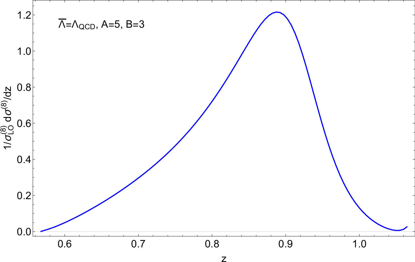
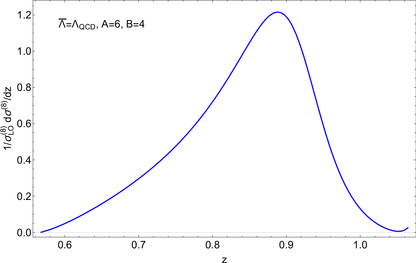
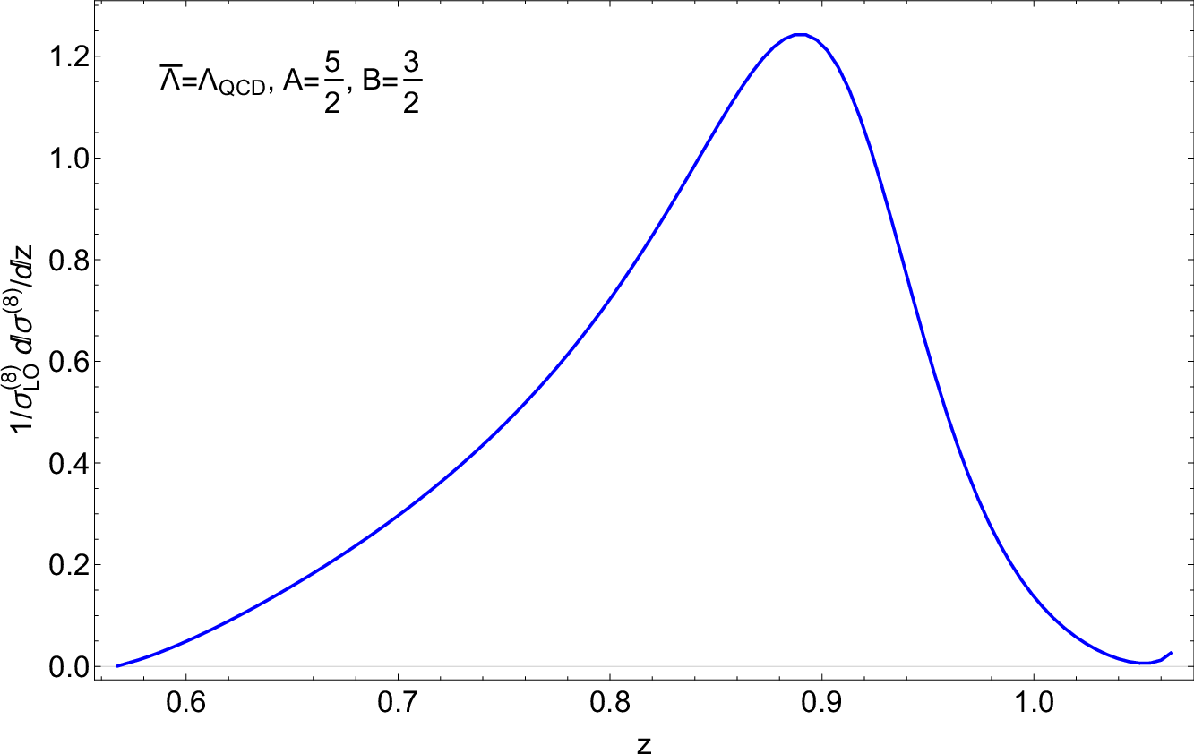
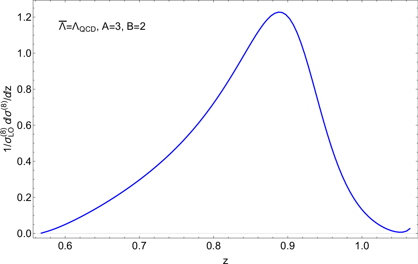
For the color-octet channel, the large endpoint logarithms have been resummed to the NLL accuracy within the SCET framework, as expounded in Sec. IV, and the endpoint divergence problem can be resolved accordingly. Away from the endpoint region, we merge the scales μS=μH=μJ=μr\mu_{S}=\mu_{H}=\mu_{J}=\mu_{r} to turn off the resummation effect. While near the endpoint, we truncate the soft scale μS\mu_{S} to around 1​GeV1\penalty\ \text{GeV}, to avoid the Landau pole. To account for the non-perturbative effects, we implement the shape function model following Ref. [33, 55]. To merge all the scales to μ\mu at small values of z, we adopted a “profile function" which smoothly turns on resummation when z is small and turns off resummation by setting all the scales equal to μ\mu. The profile function are chosen as 1±tanh⁡(15​(z′−zt​h.′))2\frac{1\pm\tanh(15(z^{\prime}-z^{\prime}_{th.}))}{2} [63]. And the explicit form of μH​(z)\mu_{H}(z) and μS​(z)\mu_{S}(z) become as μH​(z)=1−tanh⁡(15​(z′−zt​h.′))2​μr+1+tanh⁡(15​(z′−zt​h.′))2​s2​mc​(1−r)\mu_{H}(z)=\frac{1-\tanh(15(z^{\prime}-z^{\prime}_{th.}))}{2}\mu_{r}+\frac{1+\tanh(15(z^{\prime}-z^{\prime}_{th.}))}{2}\frac{s}{2m_{c}}(1-r) and μs​(z)=1−tanh⁡(15​(z′−zt​h.′))2​μr+1+tanh⁡(15​(z′−zt​h.′))2\mu_{s}(z)=\frac{1-\tanh(15(z^{\prime}-z^{\prime}_{th.}))}{2}\mu_{r}+\frac{1+\tanh(15(z^{\prime}-z^{\prime}_{th.}))}{2} where z′=(1+r)​zz^{\prime}=(1+r)z and zt​h.′z^{\prime}_{th.} is set to 0.85. We further match the NLL resummation with the NLO results to obtain the prediction for the full spectrum. The NLO ++ NLL differential cross section is plotted in Fig. 5, where four sets of parameters for the shape function are adopted, (A=5/2,B=3/2)(A=5/2,\penalty\ B=3/2), (A=3,B=2)(A=3,\penalty\ B=2), (A=5,B=3)(A=5,\penalty\ B=3) and (A=6,B=4)(A=6,\penalty\ B=4), respectively. We can see that the unphysical enhancement near the kinematic endpoint is removed after taking the resummation and shape function into account.
Refer to caption
Refer to caption
Refer to caption
Refer to caption
Figure 5: The NLO+NLL predictions for the hc​(1​P)h_{c}(1P) energy spectrum solely from the color-octet channel. We have taken different numerical inputs for the parameters AA and BB first introduced in Eq. (44).

It is curious whether and how the hc​(2​P)h_{c}(2P) meson, the first radially-excited spin-singlet PP-wave charmonium, could be observed at the Super BB factory. To reconstruct the potential hc​(2​P)h_{c}(2P) events, one potentially useful decay chain is hc​(2​P)→ηc​(2​S)​γh_{c}(2P)\to\eta_{c}(2S)\gamma, followed by ηc​(2​S)→hc​(1​P)​γ\eta_{c}(2S)\to h_{c}(1P)\gamma, hc​(1​P)→ηc​γh_{c}(1P)\to\eta_{c}\gamma, and ηc→K+​K−​π0\eta_{c}\to K^{+}K^{-}\pi^{0}. The decay chain, hc​(2​P)→ηc​(2​S)​γh_{c}(2P)\to\eta_{c}(2S)\gamma, followed by η⁡(2​S)→K​K¯​π\eta(2S)\to K\overline{K}\pi may be another good channel for hunting the hc​(2​P)h_{c}(2P). These decay channels are relatively clean, which hopefully will be helpful for hunting the elusive hc​(2​P)h_{c}(2P) state.

The theoretical formulae for hc​(1​P)h_{c}(1P) can be readily transplanted to predict the inclusive production rate of the hc​(2​P)h_{c}(2P) meson. We adopt the color-singlet LDME ⟨𝒪1hc​(2​P)​(P11)⟩=0.438​GeV5\braket{\mathcal{O}_{1}^{h_{c}(2P)}\left(\mathchoice{{\hskip 3.98613pt\hbox{$\displaystyle{P}$}^{\scriptstyle\hskip-3.98613pt\hskip-7.80904pt1\hskip 7.80904pt}_{\scriptstyle\hskip 0.0pt\hskip-7.80904pt\hskip 7.80904pt1}}}{{\hskip 3.98613pt\hbox{$\textstyle{P}$}^{\scriptstyle\hskip-3.98613pt\hskip-7.80904pt1\hskip 7.80904pt}_{\scriptstyle\hskip 0.0pt\hskip-7.80904pt\hskip 7.80904pt1}}}{{\hskip 3.40283pt\hbox{$\scriptstyle{P}$}^{\scriptscriptstyle\hskip-3.40283pt\hskip-6.16771pt1\hskip 6.16771pt}_{\scriptscriptstyle\hskip 0.0pt\hskip-6.16771pt\hskip 6.16771pt1}}}{{\hskip 3.40283pt\hbox{$\scriptscriptstyle{P}$}^{\scriptscriptstyle\hskip-3.40283pt\hskip-5.24484pt1\hskip 5.24484pt}_{\scriptscriptstyle\hskip 0.0pt\hskip-5.24484pt\hskip 5.24484pt1}}}\right)}=0.438\penalty\ \text{GeV}^{5} [20, 64]. It is rather difficult to accurately pin down the value of the color-octet LDME for hc​(2​P)h_{c}(2P), and we follow the very rough estimation based on the RGE in Ref. [10, 20], and take ⟨𝒪8hc​(2​P)​(S01)⟩≈0.013​GeV3\braket{\mathcal{O}_{8}^{h_{c}(2P)}\left(\mathchoice{{\hskip 3.98613pt\hbox{$\displaystyle{S}$}^{\scriptstyle\hskip-3.98613pt\hskip-6.70831pt1\hskip 6.70831pt}_{\scriptstyle\hskip 0.0pt\hskip-6.70831pt\hskip 6.70831pt0}}}{{\hskip 3.98613pt\hbox{$\textstyle{S}$}^{\scriptstyle\hskip-3.98613pt\hskip-6.70831pt1\hskip 6.70831pt}_{\scriptstyle\hskip 0.0pt\hskip-6.70831pt\hskip 6.70831pt0}}}{{\hskip 3.40283pt\hbox{$\scriptstyle{S}$}^{\scriptscriptstyle\hskip-3.40283pt\hskip-5.29308pt1\hskip 5.29308pt}_{\scriptscriptstyle\hskip 0.0pt\hskip-5.29308pt\hskip 5.29308pt0}}}{{\hskip 3.40283pt\hbox{$\scriptscriptstyle{S}$}^{\scriptscriptstyle\hskip-3.40283pt\hskip-4.53476pt1\hskip 4.53476pt}_{\scriptscriptstyle\hskip 0.0pt\hskip-4.53476pt\hskip 4.53476pt0}}}\right)}\approx 0.013\penalty\ \text{GeV}^{3}. With these input parameters, and ignoring the small difference in phase space integration, we then estimate the total cross section of hc​(2​P)h_{c}(2P) to be around 224​fb224\penalty\ \text{fb} at s=10.58​GeV\sqrt{s}=10.58\penalty\ \text{GeV}. When the integrated luminosity reaches 711​fb−1711\penalty\ \text{fb}^{-1} (50​ab−150\penalty\ \text{ab}^{-1}) at this specific energy, around 1.6×1051.6\times 10^{5} (1.1×1071.1\times 10^{7}) hc​(2​P)h_{c}(2P) events are expected to be produced. The energy spectrum of the hc​(2​P)h_{c}(2P) state assumes a similar shape as plotted in Fig. 5.

VI Summary

In this paper, we evaluate the NLO perturbative correction to the color-octet hch_{c} inclusive production in e+​e−e^{+}e^{-} annihilation at the Super BB factory, within the NRQCD factorization framework. We are able to deduce the analytic NLO color-octet SDC in a closed form. The NLO correction from the color-octet channel is found to be positive and important. Around 10710^{7} hc​(1​P)h_{c}(1P) and hc​(2​P)h_{c}(2P) events are expected with the projected 50​ab−150\penalty\ \text{ab}^{-1} luminosity at s=10.58​GeV\sqrt{s}=10.58\penalty\ \text{GeV} in the forthcoming Belle II experiment. It will be interesting to observe these PP-wave spin-singlet states in the inclusive production process.

Nevertheless, the hch_{c} energy spectrum predicted from the NLO calculation is plagued with the endpoint singularity, which implies the failure of the fixed-order calculation near the maximal energy of hch_{c}. With the aid of the SCET formalism, these large endpoint logarithms are resummed to the NLL accuracy. Consequently, in conjunction with the non-perturbative shape function, we obtain the well-behaved predictions for the hch_{c} energy spectrum in the entire kinematic range, which are awaiting the close examination by the forthcoming Belle II experiment.

Acknowledgments

We are grateful to Cheng-Ping Shen for several useful discussions on experimental aspects. X. L. would like to thank the Kavli Institute of Theoretical Physics in Santa Barbara for the hospitality during the completion of this manuscript. This work was supported in part by the National Natural Science Foundation of China under Grant No. 11375168, 11475188, 11621131001 (CRC110 by DGF and NSFC), and 11705092, by the Open Project Program of State Key Laboratory of Theoretical Physics under Grant No. Y4KF081CJ1, by the IHEP Innovation Grant under contract number Y4545170Y2, by the State Key Lab for Electronics and Particle Detectors.

Appendix A Analytic integration over the three-body phase space

In this Appendix, we explain how we derive the differential color-octet cross sections in Eq. (19) in DR. Recall that the three-body phase space for e+​e−→c​c¯​(S(8)01)+g​g​(q​q¯)e^{+}e^{-}\to c\bar{c}({}^{1}S_{0}^{(8)})+gg(q\bar{q}) in d=4−2​ϵd=4-2\epsilon dimensions can be expressed as [20]

∫d​Φ3\displaystyle\int{d\Phi_{3}} =cϵ​(4​π)ϵΓ⁡(1−ϵ)​(s2)1−2​ϵ​1(4​π)3​∫2​r1+rd​z​∫a−ba+bd​x1​x1−2​ϵ​(z2−4​r)−ϵ​(1−cos2⁡θ)−ϵ\displaystyle=\frac{c_{\epsilon}(4\pi)^{\epsilon}}{\Gamma(1-\epsilon)}\left(\frac{s}{2}\right)^{1-2\epsilon}\frac{1}{(4\pi)^{3}}\int_{2\sqrt{r}}^{1+r}dz\,\int_{a-b}^{a+b}dx_{1}\,x_{1}^{-2\epsilon}(z^{2}-4r)^{-\epsilon}\left(1-\cos^{2}{\theta}\right)^{-\epsilon}
=cϵ​(4​π)ϵΓ⁡(1−ϵ)​(s2)1−2​ϵ​1(4​π)3​∫2​r1+rd​z​∫a−ba+bd​x1​ 2−2​ϵ​(1+r−z)−ϵ​(x1−a+b)−ϵ​(a+b−x1)−ϵ\displaystyle=\frac{c_{\epsilon}(4\pi)^{\epsilon}}{\Gamma(1-\epsilon)}\left(\frac{s}{2}\right)^{1-2\epsilon}\frac{1}{(4\pi)^{3}}\int_{2\sqrt{r}}^{1+r}dz\,\int_{a-b}^{a+b}dx_{1}\,2^{-2\epsilon}(1+r-z)^{-\epsilon}\left(x_{1}-a+b\right)^{-\epsilon}\left(a+b-x_{1}\right)^{-\epsilon}
=cϵ​(4​π)ϵΓ⁡(1−ϵ)​s1−2​ϵ2​1(4​π)3​∫2​r1+rd​z​(1+r−z)−ϵ​∫−bbd​η​(b+η)−ϵ​(b−η)−ϵ,\displaystyle=\frac{c_{\epsilon}(4\pi)^{\epsilon}}{\Gamma(1-\epsilon)}\frac{s^{1-2\epsilon}}{2}\frac{1}{(4\pi)^{3}}\int_{2\sqrt{r}}^{1+r}dz\,(1+r-z)^{-\epsilon}\int_{-b}^{b}d{\eta}\,\left(b+\eta\right)^{-\epsilon}\left(b-\eta\right)^{-\epsilon}, (A.1)

where cϵc_{\epsilon} is introduced in Eq. (6), and θ\theta is the polar angular between 𝐤1{\bf k}_{1} and 𝐏\bf{P}:

cos⁡θ=2​(1+r−z)−x1​(2−z)x1​z2−4​r.\cos{\theta}=\frac{2(1+r-z)-x_{1}(2-z)}{x_{1}\sqrt{z^{2}-4r}}. (A.2)

In Eq. (A.1), we have introduced three auxiliary variables aa, bb and η\eta:

a=2−z2,b=z2−4​r2andη=x1−a,a=\frac{2-z}{2},\quad b=\frac{\sqrt{z^{2}-4r}}{2}\quad\text{and}\quad\eta=x_{1}-a, (A.3)

which satisfies a2−b2=1+r−za^{2}-b^{2}=1+r-z.

First, let us concentrate on the soft term ℐS​(xi,z)\mathcal{I}_{\text{S}}\left(x_{i},z\right) in Eq. (16a). Upon integrating over energy fraction of gluon 1, it will result in a single IR pole. For the sake of clarity, we discard the irrelevant perfectors in Eq. (A.1), and consider the following integral:

𝒜S≡\displaystyle\mathcal{A}_{\text{S}}\equiv ∫a−ba+bd​x1​(1+r−z)−ϵ​(x1−a+b)−ϵ​(a+b−x1)−ϵ(1+r−z−x1)2,\displaystyle\int_{a-b}^{a+b}dx_{1}\,\frac{(1+r-z)^{-\epsilon}\left(x_{1}-a+b\right)^{-\epsilon}\left(a+b-x_{1}\right)^{-\epsilon}}{\left(1+r-z-x_{1}\right)^{2}},
=\displaystyle= 1(1+r−z)1+2​ϵ​∫a−ba+bd​t​(1−a−bt)−ϵ​(a+bt−1)−ϵ(1−t)2.\displaystyle\frac{1}{(1+r-z)^{1+2\epsilon}}\int_{a-b}^{a+b}dt\,\frac{(1-\frac{a-b}{t})^{-\epsilon}(\frac{a+b}{t}-1)^{-\epsilon}}{(1-t)^{2}}. (A.4)

In the second line, we change the integration variable from x1x_{1} to tt [20],

t=1+r−zx1,t=\frac{1+r-z}{x_{1}}, (A.5)

which lies in the range

0<a−b<t<a+b<1−r.0<a-b<t<a+b<1-r. (A.6)

To explicitly identify the IR pole in 𝒜S\mathcal{A}_{\text{S}}, we can rewrite [20]

1(1+r−z)1+2​ϵ=−δ⁡(1+r−z)2​ϵ​(1−r)4​ϵ+[11+r−z]+−2​ϵ​[ln⁡(1+r−z)1+r−z]++𝒪⁡(ϵ2),\frac{1}{(1+r-z)^{1+2\epsilon}}=-\frac{\delta(1+r-z)}{2\epsilon\left(1-\sqrt{r}\right)^{4\epsilon}}+\left[\frac{1}{1+r-z}\right]_{+}-2\epsilon\left[\frac{\ln{(1+r-z)}}{1+r-z}\right]_{+}+\mathcal{O}(\epsilon^{2}), (A.7)

where the “+”-function is defined in Eq. (20).

Now the integration over tt in Eq. (A.4) is convergent, therefore one can expand the integrand in powers of ϵ\epsilon. Through the order-ϵ0\epsilon^{0}, 𝒜S\mathcal{A}_{S} bears the following form:

𝒜S={−1−r2​r​ϵ+(1−r)​[4​ln⁡(1−r)+ln⁡r]2​r}​δ​(1+r−z)+[11+r−z]+​z2−4​rr+𝒪⁡(ϵ).\displaystyle\mathcal{A}_{\text{S}}=\bigg\{-\frac{1-r}{2r\epsilon}+\frac{(1-r)\left[4\ln{\left(1-\sqrt{r}\right)}+\ln{r}\right]}{2r}\bigg\}\delta(1+r-z)+\left[\frac{1}{1+r-z}\right]_{+}\frac{\sqrt{z^{2}-4r}}{r}+\mathcal{O}(\epsilon). (A.8)

The soft-collinear term ℐSC​(xi,z)\mathcal{I}_{\text{SC}}\left(x_{i},z\right) in Eq. (16c) would result in double IR pole upon phase space integration. To facilitate the extraction of the IR poles, we first observe that ℐSC\mathcal{I}_{\text{SC}} contains the following term:

1(1+r−z)​(1+r−z−x1)=1x1​(1+r−z−x1)−1x1​(1+r−z),\frac{1}{(1+r-z)\left(1+r-z-x_{1}\right)}=\frac{1}{x_{1}\left(1+r-z-x_{1}\right)}-\frac{1}{x_{1}\left(1+r-z\right)}, (A.9)

which can be decomposed into two pieces through partial fraction.

The first term in Eq. (A.9) only leads to soft singularity. Following the trick of changing variable in Eq. (A.4), we can readily work out the following integration in DR:

𝒜S′=\displaystyle\mathcal{A}^{\prime}_{\text{S}}= ∫a−ba+bd​x1​(1+r−z)−ϵ​(x1−a+b)−ϵ​(a+b−x1)−ϵx1​(1+r−z−x1)\displaystyle\int_{a-b}^{a+b}dx_{1}\,\frac{(1+r-z)^{-\epsilon}\left(x_{1}-a+b\right)^{-\epsilon}\left(a+b-x_{1}\right)^{-\epsilon}}{x_{1}\left(1+r-z-x_{1}\right)}
=\displaystyle= 1(1+r−z)1+2​ϵ​∫a−ba+bd​t​(1−a−bt)−ϵ​(a+bt−1)−ϵt−1\displaystyle\frac{1}{(1+r-z)^{1+2\epsilon}}\int_{a-b}^{a+b}dt\,\frac{(1-\frac{a-b}{t})^{-\epsilon}(\frac{a+b}{t}-1)^{-\epsilon}}{t-1}
=\displaystyle= {−ln⁡r2​ϵ+ln⁡r4​[ln⁡r+8​ln⁡(1−r)]}​δ​(1+r−z)+[11+r−z]+​ln⁡z−z2−4​rz+z2−4​r+𝒪⁡(ϵ).\displaystyle\bigg\{-\frac{\ln{r}}{2\epsilon}+\frac{\ln{r}}{4}\left[\ln{r}+8\ln{\left(1-\sqrt{r}\right)}\right]\bigg\}\delta{(1+r-z)}+\left[\frac{1}{1+r-z}\right]_{+}\ln{\frac{z-\sqrt{z^{2}-4r}}{z+\sqrt{z^{2}-4r}}}+\mathcal{O}(\epsilon). (A.10)

The second term in Eq. (A.9) would lead to double IR pole upon integration over x1x_{1}. We then face the following integral:

𝒜SC=\displaystyle\mathcal{A}_{\text{SC}}= ∫a−ba+bd​x1​(1+r−z)−ϵ​(x1−a+b)−ϵ​(a+b−x1)−ϵx1​(1+r−z)\displaystyle\int_{a-b}^{a+b}dx_{1}\,\frac{(1+r-z)^{-\epsilon}\left(x_{1}-a+b\right)^{-\epsilon}\left(a+b-x_{1}\right)^{-\epsilon}}{x_{1}\left(1+r-z\right)}
=\displaystyle= 1(1+r−z)1+ϵ​∫a−ba+bd​x1​(x1−a+b)−ϵ​(a+b−x1)−ϵx1\displaystyle\frac{1}{(1+r-z)^{1+\epsilon}}\int_{a-b}^{a+b}dx_{1}\,\frac{\left(x_{1}-a+b\right)^{-\epsilon}\left(a+b-x_{1}\right)^{-\epsilon}}{x_{1}}
=\displaystyle= 1(1+r−z)1+ϵ​∫−bbd​η​(η+b)−ϵ​(b−η)−ϵη+a.\displaystyle\frac{1}{(1+r-z)^{1+\epsilon}}\int_{-b}^{b}d\eta\,\frac{\left(\eta+b\right)^{-\epsilon}\left(b-\eta\right)^{-\epsilon}}{\eta+a}. (A.11)

In the last step, we have switched the integration variable from x1x_{1} to η\eta, as specified in the last line of Eq. (A.1).

The integration over η\eta can be done in a straightforward way:

∫−bbd​η​(η+b)−ϵ​(b−η)−ϵη+a=π​b1−2​ϵ​Γ​(1−ϵ)​F2​1​(12,1,32−ϵ,b2a2)a​Γ​(32−ϵ)\displaystyle\int_{-b}^{b}d\eta\,\frac{\left(\eta+b\right)^{-\epsilon}\left(b-\eta\right)^{-\epsilon}}{\eta+a}=\frac{\sqrt{\pi}b^{1-2\epsilon}\Gamma(1-\epsilon){\mathchoice{{\hskip 3.98613pt\hbox{$\displaystyle{F}$}^{\scriptstyle\hskip 0.0pt\hskip-7.81946pt\hskip 7.81946pt}_{\scriptstyle\hskip-3.98613pt\hskip-7.81946pt2\hskip 7.81946pt1}}}{{\hskip 3.98613pt\hbox{$\textstyle{F}$}^{\scriptstyle\hskip 0.0pt\hskip-7.81946pt\hskip 7.81946pt}_{\scriptstyle\hskip-3.98613pt\hskip-7.81946pt2\hskip 7.81946pt1}}}{{\hskip 3.40283pt\hbox{$\scriptstyle{F}$}^{\scriptscriptstyle\hskip 0.0pt\hskip-6.14795pt\hskip 6.14795pt}_{\scriptscriptstyle\hskip-3.40283pt\hskip-6.14795pt2\hskip 6.14795pt1}}}{{\hskip 3.40283pt\hbox{$\scriptscriptstyle{F}$}^{\scriptscriptstyle\hskip 0.0pt\hskip-5.20493pt\hskip 5.20493pt}_{\scriptscriptstyle\hskip-3.40283pt\hskip-5.20493pt2\hskip 5.20493pt1}}}\left(\frac{1}{2},1;\frac{3}{2}-\epsilon;\frac{b^{2}}{a^{2}}\right)}}{a\Gamma\left(\frac{3}{2}-\epsilon\right)}
=π​b1−2​ϵ​Γ​(−ϵ)​F2​1​(12,1,1+ϵ,1−b2a2)a​Γ​(12−ϵ)+π​csc⁡(π​ϵ)​(a2−b2)−ϵ,\displaystyle=\frac{\sqrt{\pi}b^{1-2\epsilon}\Gamma(-\epsilon)\,{\mathchoice{{\hskip 3.98613pt\hbox{$\displaystyle{F}$}^{\scriptstyle\hskip 0.0pt\hskip-7.81946pt\hskip 7.81946pt}_{\scriptstyle\hskip-3.98613pt\hskip-7.81946pt2\hskip 7.81946pt1}}}{{\hskip 3.98613pt\hbox{$\textstyle{F}$}^{\scriptstyle\hskip 0.0pt\hskip-7.81946pt\hskip 7.81946pt}_{\scriptstyle\hskip-3.98613pt\hskip-7.81946pt2\hskip 7.81946pt1}}}{{\hskip 3.40283pt\hbox{$\scriptstyle{F}$}^{\scriptscriptstyle\hskip 0.0pt\hskip-6.14795pt\hskip 6.14795pt}_{\scriptscriptstyle\hskip-3.40283pt\hskip-6.14795pt2\hskip 6.14795pt1}}}{{\hskip 3.40283pt\hbox{$\scriptscriptstyle{F}$}^{\scriptscriptstyle\hskip 0.0pt\hskip-5.20493pt\hskip 5.20493pt}_{\scriptscriptstyle\hskip-3.40283pt\hskip-5.20493pt2\hskip 5.20493pt1}}}\left(\frac{1}{2},1;1+\epsilon;1-\frac{b^{2}}{a^{2}}\right)}}{a\Gamma\left(\frac{1}{2}-\epsilon\right)}+\pi\csc{(\pi\epsilon)}\left(a^{2}-b^{2}\right)^{-\epsilon}, (A.12)

where F12{}_{2}F_{1} represents the Gauss hypergeometric function. The singularity associated with the ϵ→0\epsilon\to 0 limit can be readily traced in this format, which stems from Γ⁡(−ϵ)\Gamma(-\epsilon) and csc⁡(π​ϵ)\csc(\pi\epsilon). With the aid of the package HypExp [65], we find the following expansion formula particularly useful:

F2​1​(12,1,1+ϵ,1−b2a2)=ab​(1+2​ϵ​ln⁡2​ba+b)+𝒪⁡(ϵ2).{\mathchoice{{\hskip 3.98613pt\hbox{$\displaystyle{F}$}^{\scriptstyle\hskip 0.0pt\hskip-7.81946pt\hskip 7.81946pt}_{\scriptstyle\hskip-3.98613pt\hskip-7.81946pt2\hskip 7.81946pt1}}}{{\hskip 3.98613pt\hbox{$\textstyle{F}$}^{\scriptstyle\hskip 0.0pt\hskip-7.81946pt\hskip 7.81946pt}_{\scriptstyle\hskip-3.98613pt\hskip-7.81946pt2\hskip 7.81946pt1}}}{{\hskip 3.40283pt\hbox{$\scriptstyle{F}$}^{\scriptscriptstyle\hskip 0.0pt\hskip-6.14795pt\hskip 6.14795pt}_{\scriptscriptstyle\hskip-3.40283pt\hskip-6.14795pt2\hskip 6.14795pt1}}}{{\hskip 3.40283pt\hbox{$\scriptscriptstyle{F}$}^{\scriptscriptstyle\hskip 0.0pt\hskip-5.20493pt\hskip 5.20493pt}_{\scriptscriptstyle\hskip-3.40283pt\hskip-5.20493pt2\hskip 5.20493pt1}}}\left(\frac{1}{2},1;1+\epsilon;1-\frac{b^{2}}{a^{2}}\right)}=\frac{a}{b}\left(1+2\epsilon\ln{\frac{2b}{a+b}}\right)+\mathcal{O}{(\epsilon^{2})}. (A.13)

Combining the distribution identity in Eq. (A.7), we can get

1(1+r−z)1+ϵ​π​b1−2​ϵ​Γ​(−ϵ)​F2​1​(12,1,1+ϵ,1−b2a2)a​Γ​(12−ϵ)\displaystyle\frac{1}{(1+r-z)^{1+\epsilon}}\frac{\sqrt{\pi}b^{1-2\epsilon}\Gamma(-\epsilon){\mathchoice{{\hskip 3.98613pt\hbox{$\displaystyle{F}$}^{\scriptstyle\hskip 0.0pt\hskip-7.81946pt\hskip 7.81946pt}_{\scriptstyle\hskip-3.98613pt\hskip-7.81946pt2\hskip 7.81946pt1}}}{{\hskip 3.98613pt\hbox{$\textstyle{F}$}^{\scriptstyle\hskip 0.0pt\hskip-7.81946pt\hskip 7.81946pt}_{\scriptstyle\hskip-3.98613pt\hskip-7.81946pt2\hskip 7.81946pt1}}}{{\hskip 3.40283pt\hbox{$\scriptstyle{F}$}^{\scriptscriptstyle\hskip 0.0pt\hskip-6.14795pt\hskip 6.14795pt}_{\scriptscriptstyle\hskip-3.40283pt\hskip-6.14795pt2\hskip 6.14795pt1}}}{{\hskip 3.40283pt\hbox{$\scriptscriptstyle{F}$}^{\scriptscriptstyle\hskip 0.0pt\hskip-5.20493pt\hskip 5.20493pt}_{\scriptscriptstyle\hskip-3.40283pt\hskip-5.20493pt2\hskip 5.20493pt1}}}\left(\frac{1}{2},1;1+\epsilon;1-\frac{b^{2}}{a^{2}}\right)}}{a\Gamma\left(\frac{1}{2}-\epsilon\right)}
=\displaystyle= {1ϵ2−2​ln⁡[(1−r)​(1−r)]ϵ+2​ln2​[(1−r)​(1−r)]−π26}​δ​(1+r−z)\displaystyle\bigg\{\frac{1}{\epsilon^{2}}-\frac{2\ln{\left[(1-\sqrt{r})(1-r)\right]}}{\epsilon}+2\ln^{2}{\left[(1-\sqrt{r})(1-r)\right]}-\frac{\pi^{2}}{6}\bigg\}\delta(1+r-z)
+(−1ϵ+2​ln⁡2−z+z2−4​r2)​[11+r−z]++[ln⁡(1+r−z)1+r−z]++𝒪⁡(ϵ),\displaystyle+\left(-{1\over\epsilon}+2\ln{2-z+\sqrt{z^{2}-4r}\over 2}\right)\left[\frac{1}{1+r-z}\right]_{+}+\left[\frac{\ln(1+r-z)}{1+r-z}\right]_{+}+\mathcal{O}(\epsilon), (A.14a)
1(1+r−z)1+ϵ​π​csc⁡(π​ϵ)​(a2−b2)−ϵ\displaystyle\frac{1}{(1+r-z)^{1+\epsilon}}\pi\csc(\pi\epsilon)\left(a^{2}-b^{2}\right)^{-\epsilon} (A.14b)
=\displaystyle= {−12​ϵ2+2​ln⁡(1−r)ϵ−4​ln2⁡(1−r)−π212}​δ​(1+r−z)+1ϵ​[11+r−z]+−2​[ln⁡(1+r−z)1+r−z]++𝒪⁡(ϵ).\displaystyle\bigg\{-\frac{1}{2\epsilon^{2}}+\frac{2\ln\left(1-\sqrt{r}\right)}{\epsilon}-4\ln^{2}\left(1-\sqrt{r}\right)-\frac{\pi^{2}}{12}\bigg\}\delta(1+r-z)+\frac{1}{\epsilon}\left[\frac{1}{1+r-z}\right]_{+}-2\left[\frac{\ln(1+r-z)}{1+r-z}\right]_{+}+\mathcal{O}(\epsilon).

Adding these two pieces together, we arrive at the final expression for 𝒜SC\mathcal{A}_{\text{SC}}:

𝒜SC=\displaystyle\mathcal{A}_{\text{SC}}= {12​ϵ2−2​ln⁡(1−r)ϵ−4​ln2⁡(1−r)+2​ln2​[(1−r)​(1−r)]−π24}​δ​(1+r−z)\displaystyle\bigg\{\frac{1}{2\epsilon^{2}}-\frac{2\ln(1-r)}{\epsilon}-4\ln^{2}\left(1-\sqrt{r}\right)+2\ln^{2}{\left[(1-\sqrt{r})(1-r)\right]}-\frac{\pi^{2}}{4}\bigg\}\delta(1+r-z)
+2​ln⁡(2−z+z2−4​r2)​[11+r−z]+−[ln⁡(1+r−z)1+r−z]++𝒪⁡(ϵ).\displaystyle+2\ln{\left(\frac{2-z+\sqrt{z^{2}-4r}}{2}\right)}\left[\frac{1}{1+r-z}\right]_{+}-\left[\frac{\ln{(1+r-z)}}{1+r-z}\right]_{+}+\mathcal{O}(\epsilon). (A.15)

The occurrence of double IR pole is as anticipated, by examining the pole structure of Eq. (16c).

References

  • [1] T. A. Armstrong et al., Phys. Rev. Lett. 69, 2337 (1992). doi:10.1103/PhysRevLett.69.2337
  • [2] M. Andreotti et al., Phys. Rev. D 72, 032001 (2005). doi:10.1103/PhysRevD.72.032001
  • [3] J. L. Rosner et al. [CLEO Collaboration], Phys. Rev. Lett. 95, 102003 (2005) doi:10.1103/PhysRevLett.95.102003 [hep-ex/0505073].
  • [4] P. Rubin et al. [CLEO Collaboration], Phys. Rev. D 72, 092004 (2005) doi:10.1103/PhysRevD.72.092004 [hep-ex/0508037].
  • [5] M. Ablikim et al. [BESIII Collaboration], Phys. Rev. Lett. 104, 132002 (2010) doi:10.1103/PhysRevLett.104.132002 [arXiv:1002.0501 [hep-ex]].
  • [6] M. Ablikim et al. [BESIII Collaboration], Phys. Rev. D 86, 092009 (2012) doi:10.1103/PhysRevD.86.092009 [arXiv:1209.4963 [hep-ex]].
  • [7] C. Patrignani et al. [Particle Data Group], Chin. Phys. C 40, no. 10, 100001 (2016). doi:10.1088/1674-1137/40/10/100001
  • [8] I. Adachi et al. [Belle Collaboration], Phys. Rev. Lett. 108, 032001 (2012) doi:10.1103/PhysRevLett.108.032001 [arXiv:1103.3419 [hep-ex]].
  • [9] W. E. Caswell and G. P. Lepage, Phys. Lett. 167B, 437 (1986). doi:10.1016/0370-2693(86)91297-9
  • [10] G. T. Bodwin, E. Braaten and G. P. Lepage, Phys. Rev. D 51, 1125 (1995) Erratum: [Phys. Rev. D 55, 5853 (1997)] doi:10.1103/PhysRevD.55.5853, 10.1103/PhysRevD.51.1125 [hep-ph/9407339].
  • [11] N. Brambilla et al., Eur. Phys. J. C 71, 1534 (2011) doi:10.1140/epjc/s10052-010-1534-9 [arXiv:1010.5827 [hep-ph]].
  • [12] V. A. Novikov, L. B. Okun, M. A. Shifman, A. I. Vainshtein, M. B. Voloshin and V. I. Zakharov, Phys. Rept. 41, 1 (1978). doi:10.1016/0370-1573(78)90120-5
  • [13] J. Z. Li, Y. Q. Ma and K. T. Chao, Phys. Rev. D 88, no. 3, 034002 (2013) doi:10.1103/PhysRevD.88.034002 [arXiv:1209.4011 [hep-ph]].
  • [14] G. T. Bodwin, E. Braaten, T. C. Yuan and G. P. Lepage, Phys. Rev. D 46, R3703 (1992) doi:10.1103/PhysRevD.46.R3703 [hep-ph/9208254].
  • [15] M. Beneke, F. Maltoni and I. Z. Rothstein, Phys. Rev. D 59, 054003 (1999) doi:10.1103/PhysRevD.59.054003 [hep-ph/9808360].
  • [16] S. Fleming and T. Mehen, Phys. Rev. D 58, 037503 (1998) [AIP Conf. Proc. 452, no. 1, 101 (1998)] doi:10.1063/1.57084, 10.1103/PhysRevD.58.037503 [hep-ph/9801328].
  • [17] K. Sridhar, Phys. Lett. B 674, 36 (2009) doi:10.1016/j.physletb.2009.02.051 [arXiv:0812.0474 [hep-ph]].
  • [18] C. F. Qiao, D. L. Ren and P. Sun, Phys. Lett. B 680, 159 (2009) doi:10.1016/j.physletb.2009.08.047 [arXiv:0904.0726 [hep-ph]].
  • [19] J. X. Wang and H. F. Zhang, J. Phys. G 42, no. 2, 025004 (2015) doi:10.1088/0954-3899/42/2/025004 [arXiv:1403.5944 [hep-ph]].
  • [20] Y. Jia, W. L. Sang and J. Xu, Phys. Rev. D 86, 074023 (2012) doi:10.1103/PhysRevD.86.074023 [arXiv:1206.5785 [hep-ph]].
  • [21] J. X. Wang and H. F. Zhang, Phys. Rev. D 86, 074012 (2012) doi:10.1103/PhysRevD.86.074012 [arXiv:1207.2416 [hep-ph]].
  • [22] G. Chen, X. G. Wu, Z. Sun, X. C. Zheng and J. M. Shen, Phys. Rev. D 89, no. 1, 014006 (2014) doi:10.1103/PhysRevD.89.014006 [arXiv:1311.2735 [hep-ph]].
  • [23] L. B. Chen, J. Jiang and C. F. Qiao, Chin. Phys. C 39, no. 10, 103101 (2015) doi:10.1088/1674-1137/39/10/103101 [arXiv:1505.00382 [hep-ph]].
  • [24] R. Zhu, Phys. Rev. D 92, no. 7, 074017 (2015) doi:10.1103/PhysRevD.92.074017 [arXiv:1507.02031 [hep-ph]].
  • [25] F. Feng, S. Ishaq, Y. Jia and J. Y. Zhang, arXiv:1712.09986 [hep-ph].
  • [26] A. Abulencia et al. [CDF Collaboration], Phys. Rev. Lett. 99, 132001 (2007) doi:10.1103/PhysRevLett.99.132001 [arXiv:0704.0638 [hep-ex]].
  • [27] R. Aaij et al. [LHCb Collaboration], Eur. Phys. J. C 71, 1645 (2011) doi:10.1140/epjc/s10052-011-1645-y [arXiv:1103.0423 [hep-ex]].
  • [28] G. Aad et al. [ATLAS Collaboration], Nucl. Phys. B 850, 387 (2011) doi:10.1016/j.nuclphysb.2011.05.015 [arXiv:1104.3038 [hep-ex]].
  • [29] V. Khachatryan et al. [CMS Collaboration], Eur. Phys. J. C 71, 1575 (2011) doi:10.1140/epjc/s10052-011-1575-8 [arXiv:1011.4193 [hep-ex]].
  • [30] B. Abelev et al. [ALICE Collaboration], Phys. Rev. Lett. 108, 082001 (2012) doi:10.1103/PhysRevLett.108.082001 [arXiv:1111.1630 [hep-ex]].
  • [31] T. K. Pedlar et al. [CLEO Collaboration], Phys. Rev. Lett. 107, 041803 (2011) doi:10.1103/PhysRevLett.107.041803 [arXiv:1104.2025 [hep-ex]].
  • [32] M. Ablikim et al. [BESIII Collaboration], Phys. Rev. Lett. 118, no. 9, 092002 (2017) doi:10.1103/PhysRevLett.118.092002 [arXiv:1610.07044 [hep-ex]].
  • [33] S. Fleming, A. K. Leibovich and T. Mehen, Phys. Rev. D 68, 094011 (2003) doi:10.1103/PhysRevD.68.094011 [hep-ph/0306139].
  • [34] C. W. Bauer, S. Fleming and M. E. Luke, Phys. Rev. D 63, 014006 (2000) doi:10.1103/PhysRevD.63.014006 [hep-ph/0005275].
  • [35] C. W. Bauer, S. Fleming, D. Pirjol and I. W. Stewart, Phys. Rev. D 63, 114020 (2001) doi:10.1103/PhysRevD.63.114020 [hep-ph/0011336].
  • [36] C. W. Bauer and I. W. Stewart, Phys. Lett. B 516, 134 (2001) doi:10.1016/S0370-2693(01)00902-9 [hep-ph/0107001].
  • [37] C. W. Bauer, D. Pirjol and I. W. Stewart, Phys. Rev. D 65, 054022 (2002) doi:10.1103/PhysRevD.65.054022 [hep-ph/0109045].
  • [38] C. W. Bauer, S. Fleming, D. Pirjol, I. Z. Rothstein and I. W. Stewart, Phys. Rev. D 66, 014017 (2002) doi:10.1103/PhysRevD.66.014017 [hep-ph/0202088].
  • [39] M. Beneke, A. P. Chapovsky, M. Diehl and T. Feldmann, Nucl. Phys. B 643, 431 (2002) doi:10.1016/S0550-3213(02)00687-9 [hep-ph/0206152].
  • [40] G. C. Nayak, J. W. Qiu and G. F. Sterman, Phys. Lett. B 613, 45 (2005) doi:10.1016/j.physletb.2005.03.031 [hep-ph/0501235].
  • [41] G. C. Nayak, J. W. Qiu and G. F. Sterman, Phys. Rev. D 72, 114012 (2005) doi:10.1103/PhysRevD.72.114012 [hep-ph/0509021].
  • [42] A. Petrelli, M. Cacciari, M. Greco, F. Maltoni and M. L. Mangano, Nucl. Phys. B 514, 245 (1998) doi:10.1016/S0550-3213(97)00801-8 [hep-ph/9707223].
  • [43] G. T. Bodwin, X. Garcia i Tormo and J. Lee, Phys. Rev. D 81, 114014 (2010) doi:10.1103/PhysRevD.81.114014 [arXiv:1003.0061 [hep-ph]].
  • [44] W. Y. Keung, Phys. Rev. D 23, 2072 (1981). doi:10.1103/PhysRevD.23.2072
  • [45] T. Hahn, Comput. Phys. Commun. 140, 418 (2001) doi:10.1016/S0010-4655(01)00290-9 [hep-ph/0012260].
  • [46] V. Shtabovenko, R. Mertig and F. Orellana, Comput. Phys. Commun. 207, 432 (2016) doi:10.1016/j.cpc.2016.06.008 [arXiv:1601.01167 [hep-ph]].
  • [47] B. W. Harris and J. F. Owens, Phys. Rev. D 65, 094032 (2002) doi:10.1103/PhysRevD.65.094032 [hep-ph/0102128].
  • [48] F. Feng, Comput. Phys. Commun. 183, 2158 (2012) doi:10.1016/j.cpc.2012.03.025 [arXiv:1204.2314 [hep-ph]].
  • [49] A. V. Smirnov, Comput. Phys. Commun. 189, 182 (2015) doi:10.1016/j.cpc.2014.11.024 [arXiv:1408.2372 [hep-ph]].
  • [50] T. Hahn and M. Perez-Victoria, Comput. Phys. Commun. 118, 153 (1999) doi:10.1016/S0010-4655(98)00173-8 [hep-ph/9807565].
  • [51] Y. J. Zhang, Y. Q. Ma, K. Wang and K. T. Chao, Phys. Rev. D 81, 034015 (2010) doi:10.1103/PhysRevD.81.034015 [arXiv:0911.2166 [hep-ph]].
  • [52] S. Fleming, A. K. Leibovich, T. Mehen and I. Z. Rothstein, Phys. Rev. D 86, 094012 (2012) doi:10.1103/PhysRevD.86.094012 [arXiv:1207.2578 [hep-ph]].
  • [53] Z. B. Kang, Y. Q. Ma, J. W. Qiu and G. Sterman, Phys. Rev. D 90, no. 3, 034006 (2014) doi:10.1103/PhysRevD.90.034006 [arXiv:1401.0923 [hep-ph]].
  • [54] Y. Q. Ma, J. W. Qiu, G. Sterman and H. Zhang, Phys. Rev. Lett. 113, no. 14, 142002 (2014) doi:10.1103/PhysRevLett.113.142002 [arXiv:1407.0383 [hep-ph]].
  • [55] A. K. Leibovich, Z. Ligeti and M. B. Wise, Phys. Lett. B 539, 242 (2002) doi:10.1016/S0370-2693(02)02097-X [hep-ph/0205148].
  • [56] G. T. Bodwin, J. Lee and C. Yu, Phys. Rev. D 77, 094018 (2008) doi:10.1103/PhysRevD.77.094018 [arXiv:0710.0995 [hep-ph]].
  • [57] T. van Ritbergen, J. A. M. Vermaseren and S. A. Larin, Phys. Lett. B 400, 379 (1997) doi:10.1016/S0370-2693(97)00370-5 [hep-ph/9701390].
  • [58] K. G. Chetyrkin, J. H. Kuhn and M. Steinhauser, Comput. Phys. Commun. 133, 43 (2000) doi:10.1016/S0010-4655(00)00155-7 [hep-ph/0004189].
  • [59] P. L. Cho and A. K. Leibovich, Phys. Rev. D 53, 150 (1996) doi:10.1103/PhysRevD.53.150 [hep-ph/9505329].
  • [60] Y. Q. Ma, K. Wang and K. T. Chao, Phys. Rev. D 83, 111503 (2011) doi:10.1103/PhysRevD.83.111503 [arXiv:1002.3987 [hep-ph]].
  • [61] B. Gong, L. P. Wan, J. X. Wang and H. F. Zhang, Phys. Rev. Lett. 110, no. 4, 042002 (2013) doi:10.1103/PhysRevLett.110.042002 [arXiv:1205.6682 [hep-ph]].
  • [62] P. L. Cho and A. K. Leibovich, Phys. Rev. D 53, 6203 (1996) doi:10.1103/PhysRevD.53.6203 [hep-ph/9511315].
  • [63] X. Liu and F. Petriello, Phys. Rev. D 87, no. 9, 094027 (2013) doi:10.1103/PhysRevD.87.094027 [arXiv:1303.4405 [hep-ph]].
  • [64] E. J. Eichten and C. Quigg, Phys. Rev. D 52, 1726 (1995) doi:10.1103/PhysRevD.52.1726 [hep-ph/9503356].
  • [65] T. Huber and D. Maitre, Comput. Phys. Commun. 178, 755 (2008) doi:10.1016/j.cpc.2007.12.008 [arXiv:0708.2443 [hep-ph]].