An Analysis of the Convergence of Stochastic Lagrangian/Eulerian Spray Simulations
Abstract
This work derives how the convergence of stochastic Lagrangian/Eulerian simulations depends on the number of computational parcels, particularly for the case of spray modeling. A new, simple, formula is derived that can be used for managing the numerical error in two or three dimensional computational studies. For example, keeping the number of parcels per cell constant as the mesh is refined yields an order one-half convergence rate in transient spray simulations. First order convergence would require a doubling of the number of parcels per cell when the cell size is halved. Second order convergence would require increasing the number of parcels per cell by a factor of eight. The results show that controlling statistical error requires dramatically larger numbers of parcels than have typically been used, which explains why convergence has been so elusive.
Keywords:
convergence , Lagrangian , Eulerian , spray , CFD1 Introduction to the Problem
The computational fluid dynamics community expects numerical schemes to be consistent, i.e. they should converge to the exact solution as resolution is increased. Without this assurance, the modeler can wander aimlessly, confused by pathological numerical errors. The present work will identify a simple rule that governs convergence and will bring Lagrangian/Eulerian spray simulation closer to modern standards of simulation quality. The mathematical analysis is intended to also benefit other forms of Lagrangian/Eulerian simulations, such as bubbly or particle-laden flow.
The first step is to identify what is and what is not understood. The typical parts of a Lagrangian/Eulerian spray computation can be categorized as follows:
- 1.
Gas phase equations: The gas phase conservation equations, excluding source terms for interaction with the spray, solved in an Eulerian frame of reference
- 2.
Particle tracking: The governing ordinary differential equations that describe the evolution of the tracked particles, solved in a Lagrangian frame of reference
- 3.
Gas to liquid coupling: The interpolation of gas phase quantities to the location of the spray parcels
- 4.
Liquid to gas coupling: The agglomeration of the scattered point particle effects into source terms in the continuous phase equations
The first item is well understood. The second category includes the models that describe the evolution of droplets as they move in the Lagrangian reference frame. Are et al. [1] provided analysis for the basic equations of spray motion. Spray breakup has not been analyzed but is expected, for at least basic breakup models, to behave as ordinary differential equations (ODEs) which are well understood. Droplet collision is beyond the scope of this paper and has been studied elsewhere [2, 3]. Gas to liquid coupling is equivalent to interpolation and was also analyzed by Are et al.
The final item, representing the effect of the liquid phase on the gas phase, has proven to be the most challenging. Here, the numerical methods accumulate information from the liquid phase about mass, momentum, energy, and species contributions to the gas phase. These methods must contend with the fact that parcels are not collocated with gas phase nodes or finite volume cell centers. Further, because of the limited number of parcels used in spray computations, there is a statistical uncertainty in these terms.
Because of this statistical uncertainty, refinement of gas phase solution without adequately refining the Lagrangian solution by increasing the number of computational parcels can actually result in a less accurate answer. Early work by Subramaniam and O’Rourke [4] concluded that the convergence of spray simulations was conditional on employing a sufficient number of parcels. Subsequent analysis by Schmidt [5] saw similar trends. If the number of parcels is held constant while the mesh is refined, the error begins to increase after passing an optimum, as shown in Fig. 1.

There have been several past investigations of liquid to gas coupling. The work of Stalsberg-Zarling et al. [6] applied Lagrange polynomial interpolation to interphase coupling in order to produce a more stable, less mesh-dependent simulation. The work of Garg et al. [7] used several problems that admitted analytical solutions in order to empirically study the convergence rate of fairly sophisticated coupling schemes. For completeness, they included statistical factors in their tests by varying the number of parcels per cell. In order to understand the behavior and causes of the error, they modeled deterministic, bias, and statistical contributions using a framework suggested by Dreeben and Pope [8].
The work of Garg et al. judged the efficacy of these liquid to gas coupling schemes based on empirical tests. In later work, Garg et al. [9] developed a parcel number density control system to moderate statistical error and, with the help of a sophisticated liquid-to-gas source estimation scheme, produced convergence of a fully-coupled Lagrangian/Eulerian calculation. Their success strongly supports the notion that the distribution of sources from the Lagrangian phase to the Eulerian is the crux of controlling overall error.
In contrast, the work of Are et al. excluded considerations of statistical error in both their analytical and empirical tests. The analysis took the limit of an infinite number of parcels, while the empirical tests used arbitrary, large numbers of parcels. They succeeded in showing theoretically, for each of the elements listed above, how to achieve second order accuracy. They then combined these elements into a full Lagrangian/Eulerian simulation and demonstrated second order convergence. Later, Schmidt [5] studied how second order and higher accuracy schemes converge considering both spatial and statistical error. However, Schmidt only considered liquid-to-gas coupling and only for fixed numbers of parcels per cell.
The outstanding question that has never been answered is:“In a Lagrangian/Eulerian simulation, how fast must the number of parcels increase in order to observe convergence during mesh refinement?” Without knowing the answer, one cannot reliably demonstrate spray calculation convergence. The present work derives a recipe that answers this question and performs demonstrations in order to empirically confirm the predictions.
This effort will add to the body of literature that has empirically studied convergence, such as Senecal et al. [10]. These studies have proceeded without analysis to provide guidance. Senecal et al. is an example where the authors successfully achieved convergence by a combination of careful numerical methods and employing a substantial number of computational parcels. In a subsequent section of this paper, their approach will be compared to the rule which we derive.
2 Analysis of a Single Time Step
Our analysis examines the calculation of particle to gas source terms as a function of location in a dimensional space. The magnitude of the sources in this analysis is determined by the gas-to-particle coupling, reducing the particle-to-gas coupling to a determination of how the sources are to be distributed on the gas phase mesh. Consequentially, the distribution of sources can be represented by a density function which is estimated from non-uniformly spaced parcels (See Pai and Subramaniam [11] for an investigation of discrete particle representations of smooth distribution functions). For each continuous phase cell, the contributions of the local parcel sample is summed using a kernel with compact support.
Our approach will be to construct an estimate of the combined error due to statistical and spatial contributions. This estimate will be dependent on both the number of parcels and the level of spatial resolution. We will then assert that the number of parcels must be tied to the cell size by a simple power law relation, which then results in an error estimate that is only a function of cell size. Finally, we will calculate the convergence rate of this error.
The analysis begins with our representation of the kernel used to connect parcel contributions to the source term. As reviewed by Garg et al. [7] and Schmidt [5] there are several approaches that can achieve varying degrees of spatial accuracy or reduced statistical error. The simplest and most common approach in Lagrangian/Eulerian spray simulations is the nearest-node kernel. This treatment, in a finite volume context, is simply: if a parcel resides in a cell, then all of the contributions from the parcel go the gas phase equation for that cell.
The nearest node kernel can be represented as a function that depends on the dimensionless distance from the center of the cell in a -dimensional Cartesian space, where is the index of a dimension.
| (1) |
The present work will consider the simplified case where the kernel is the same in each dimension and the mesh spacing is uniform and constant in each dimension, and so the subscript is dropped. The argument of the kernel, , is defined for the parcel below, where is the location of the nearest cell center. Similarly, is the location of the parcel. The symbol represents a unit vector in the direction.
| (2) |
The numerical estimate of the source term distribution function, , is the result of applying the kernel in all dimensions to all parcels. Here, represents the number of parcels in the entire domain.
| (3) |
The mean square error, , is defined as the square of the difference between the true source distribution function, , and the expected numerical value, , produced by Eqn. 3. Here, we can build on prior efforts to understand the related problem of finding the optimal kernel for estimating density functions. Epanechnikov [12] calculated the mean square error for a dimensional space and a general kernel.
| (4) |
The first term represents the statistical error, which depends on the variance of the kernel and can be calculated in each dimension separately for the nearest node kernel [13].
| (5) |
Inserting the nearest-node kernel definition in the mean square error estimate gives the specific result in Eqn. 6. It is comprised of two terms, the first representing the stochastic error in the source term and the second representing the spatial error. In the case considered here, for very small the first term will dominate unless increases sufficiently fast with decreasing cell size. For situations where the cell size is large compared to the length scale established by the second derivative, the spatial error term may instead dominate.
| (6) |
The mean square error is a point-wise measurement that can be assessed over the whole domain using the norm. For a discrete simulation, is calculated as follows.
| (7) |
Now the goal is to find how the number of parcels in the domain, , must depend on such that error measured by decreases at a desired rate. The relationship between and the cell size is stipulated as a power law relationship as given by Eqn. 8
| (8) |
where is an arbitrary constant. The parameter controls the rate at which the number of parcels must increase with mesh refinement. For example, the case of indicates no increase in the numbers of parcels with mesh refinement. Setting means that the number of parcels per cell remains constant with mesh refinement.
Combining the last three equations gives the following result.
| (9) |
where the integer indexes the dimensions up to in the second term. Allowing to become arbitrarily small gives the limiting behavior:
| (10) |
The first term under the radical represents statistical error and the second term represents spatial error. These two sources are in contrast to the three error contributions suggested by Dreeben and Pope [8]. The present analysis results in an unbiased estimation of the source terms.
However, this analysis should not be interpreted as a dismissal of bias error. The present analysis does not include the full set of evolution equations, so the potential still remains for bias to appear through feedback and propagation in the droplet motion calculation and the Navier-Stokes equations.
The quantities inside the two integrals are consequences of the spatial variation of the source term and are not impacted by the resolution or parcel number. For example, the integral of over the domain is simply the total amount of the source, mass, momentum, or energy, transferred per unit time into the Eulerian phase.
The main focus of our attention is the asymptotic behavior of the expression for small . In such situations the statistical error represented by the first term dominates because the exponent on , , is usually less than the exponent 4 that is present in the spatial error term. Contrasting Eqn. 10 to Eqn. 6 provides some interpretation of this statistical error term. We see in Eqn. 6 the typical error that is evident in Monte-Carlo sampling calculations. However, when we recognize that the sample size must be tied to the mesh resolution for the nearest-node kernel, the behavior of this term changes. In Eqn. 10 we see that has been replaced by a dependence on . The dependence on dimension is also a consequence of the definition of source terms – sources are an intensity: a source per length, per area, or per volume.
The rightmost term under the radical in Eqn. 10 is not sufficent for second-order spatial accuracy. For CFD codes that do not meet the requirements for second-order spatial accuracy, the second order spatial error in Eqn. 10 may be over-shadowed by other first-order errors in other parts of the spray calculation. For simulations involving very large numbers of parcels or coarse mesh resolution, the spatial error will dominate. The work of Are et al. demonstrated the second-order convergence of two-dimensional spray calculations in the limit of large numbers of parcels [1].
The convergence of the first term and the second term in Eqn. 10 are different, with the rate of convergence at very small usually limited by the first term for reasons of computational cost. In the well-resolved limit, we neglect the second term and observe that the power law behavior of the norm as a function of is one-half of . If we denote the power law behavior of as the convergence rate , then the following rule is deduced for .
| (11) |
Put simply, for a convergence rate in a dimensional calculation of the sources at a single time step, the number of parcels is governed by the exponent . This expression can be used to calculate the behavior of the number of parcels per cell, , for a convergence rate .
| (12) |
One interesting consequence of this expression is that, for the simple kernel considered here, if the number of parcels per cell is held constant as the mesh resolution is increased, the predicted convergence rate is zero, meaning convergence will not occur for a single time step. The situation of a fixed number of parcels per cell corresponds to , where the statistical error term in Eqn. 10 does not diminish.
Physically, this result is a consequence of the source terms being a density function, calculated per unit area or volume, and depending on the dimensionality of the problem.
In general, Eqns. 11 and 12 indicate that the number of parcels per cell must increase dramatically in order to observe convergence in a multi-dimensional CFD calculation. For second-order convergence (e.g. ) in a three-dimensional calculation, the exponent produced by Eqn. 11 would be 7. Referring back to Eqn. 8, this means that the number of parcels must increase with the inverse of to the seventh power.
3 A Simplified Demonstration of a Single Time step
For demonstrating convergence, a test case was employed that permits an analytical solution for the sources at an instant in time. In this test case, particles were stochastically distributed over a unit square with a spatially varying number density proportional to the product of and . Each particle contributed a uniform amount to the source term calculation, but the spatial variation in number density created a source as a function of and [5]. The number of parcels was governed by Eqn. 11 in order to test the theory.
The sources were compared to an exact solution and an error norm was calculated using an analytical expression. The number of parcels in the domain was set according to Eqn. 8 with equaling .
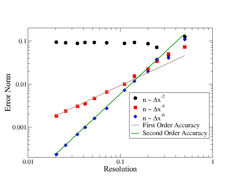
Figure 2 shows that, as predicted by Eqn. 11, second order accuracy requires the number of parcels to increase to the sixth power of the reciprocal of mesh spacing. The first order accuracy with is also predicted by Eqn. 11. As previously derived by Schmidt [5] convergence rates beyond second order are not possible unless the kernel weighting changes sign. For such higher-order kernels, however, the statistical errors may become more pronounced.
Note that for , where the number of parcels per cell remains constant, the resulting rate of convergence is predicted to be zero, indicating a failure to converge. This prediction is consistent with the empirical results of Fig. 2. Thus it is shown that, unless one uses special techniques to moderate statistical error, as in Garg et al. [9], a constant number of parcels per cell is not sufficient to obtainin convergence. Again, this is consistent with Eqn. 12 for a value of of zero.
The results do not show the characteristic minimum present in Fig. 1. The curve plotted in Fig. 1 corresponds to the case where and the number of parcels in the entire domain remains fixed. Obviously, under such conditions, convergence is not possible.
The other important lesson of this test is the magnitude of the cost of achieving convergence. For the second order convergence test, the number of parcels per cell increased from eight to over forty-eight million as the spatial resolution was increased by a factor of fifty. As one can see from Eqn. 11, the cost of three-dimensional convergence is even higher. Fortunately, transient simulations will benefit from the repeated use of parcels as they persist over multiple time steps.
4 Extension to Transient Spray Simulations
The prior analysis applies to the calculation of sources at a single fixed time. There are several transient scenarios that could be considered. In a quasi-steady scenario, the parcels are injected at the same average rate at which they leave the domain. Another scenario is of transient injection, where the domain initially has no parcels, but rather parcels are injected over a finite time.
The latter case will be considered here, as it is particularly germane to transient spray calculations. It will be assumed that the time of injection is less than the parcel residence time, so that no parcels leave the domain. We will analyze the cumulative effect of the gas/spray coupling over a time that is equal to the time of injection.
The critical extension from the previous analysis to transient sprays is to recognize that a parcel is re-used in every subsequent time-step for estimating sources. This produces a sample size that is much larger than the number of parcels injected over the total duration of injection. If a fixed number of parcels is injected every time step, after steps the total sample size becomes the sum of a series, as given in Eqn. 13.
| (13) |
This analysis presumes that the quantity of interest is the result of the cumulative effect of the transient injection. Thus the sample size is the cumulative sum of parcels in the domain over all time steps. Hence, the first term in the series corresponds to the first time step after the start of injection, the second term corresponds to the second time step, etc.
Consider an injection over a duration, . If the Courant-Friedrichs-Lewy (CFL) number is constant and equal to unity then the number of time steps can be eliminated in the following expression for sample size. Here, is the velocity scale that appears in the CFL number, which is treated as a constant. It is assumed that no parcels exit the calculation, and thus the number of parcels is the product of the number of steps, , and .
| (14) |
We see that the sample size is no longer simply the number of parcels , but is instead a more complicated expression that depends on the mesh resolution. This expression is now substituted into Eq. 10, where the sample size replaces . The result is more favorable to observing convergence than the single time-step result, but still represents considerable expense.
| (15) |
As before, for the case where the first term dominates the error, a rule for transient CFD convergence can be obtained in the limit of a well-resolved simulation. The convergence rate of the norm follows the exponent of the first term, one half of the quantity . This is rearranged to produce Eqn. 16:
| (16) |
Compared to the results for a single time step, the result of Eqn. 16 produces a value of that is reduced by unity. Because stochastic fluctuations are averaged over a large number of time steps, transient calculations are less expensive to converge. This result assumes the calculation proceeds with a constant time step and invokes the Courant number to express the number of steps as a function of . This extra factor is responsible for the in Eqn. 16. Note also that this improvement in convergence is only expected for time-averaged quantities considered for the injection duration .
A simple example will elucidate the predictions of this analysis. Consider the relatively simple case of refining a three-dimensional mesh containing cubic cells. If the cell size is halved, the number of cells increases by eight. To obtain first-order convergence in such an oct-tree refinement scheme, Eqn. 16 indicates that the value of is four and thus the total number of parcels must increase by a factor of sixteen with each level of refinement. This rule may be expressed more conveniently using the number of parcels per cell, .
| (17) |
This expression indicates that keeping the number of parcels per cell constant as the mesh is refined yields an order one-half convergence rate in transient spray simulations. First order convergence would require a doubling of the number of parcels per cell if the cell size is halved. Second order convergence would require increasing the number of parcels per cell by a factor of eight.
Note that a fundamental difference between the single-step result and the transient CFD situation is that the strategy of maintaining a constant number of parcels per cell will converge for transient calculations. Repeating the thought-experiment for refining cubic cells, if a value of is used, Eqn. 16 indicates that the rate of convergence will be one-half.
This result gives a new perspective on the results of Senecal et al. [10]. In their convergence study, they considered a diesel spray emanating from a 90 micron orifice. They started with a 2 mm mesh resolution and applied oct-tree refinement down to a resolution of 31 microns over seven increasingly refined runs. For the first five runs, they kept the number of parcels per cell constant, thus increasing the number of parcels in the computation by a factor of eight. For the final two runs, they increased the number of parcels more slowly, but still used a very large number (21 million for the finest mesh). Their observations indicated that their results were converging.
It is likely that the spatial error term in Eqn. 15 was still the limiting term in their computations. This is a logical consequence of two important details in their study. The first is that even the finest mesh was only one-third the initial spray width. Thus, the spatial error term in Eqn. 15 was significant. As a comparison, their finest resolution would roughly correspond to the coarsest point in Fig. 2. Secondly, regardless of the rate of increase, their large number of parcels would help keep the size of the first term in Eqn. 10 relatively small, corresponding to a large value of . In any case, the analysis of the present work predicts that their calculations should converge.
5 A Transient Demonstration
A quantitative test of convergence rate was performed using STAR-CCM+ version 12.06. An injector was specifically constructed in order to ensure smoothness in all spatial distributions. A typical injection has an abrupt change in number density at the edge of the orifice where the probability of injecting a parcel goes to zero abruptly as the radial location reaches the orifice radius. A probability distribution function proportional to the cosine of distance from the injection center of injection was used to ensure a smooth transition.
For similar reasons, a sine function was used for the mass flow rate curve. Additionally the initial time step of each parcel was stochastically varied immediately after injection in order to uniformly spatially sample the volume downstream of the injection location. For the sake of simplicity no breakup, turbulence, or collision sub-models were used.
The nominal injector radius was 1 and the computational domain was a 2x2x3 hexahedron, where the direction of injection was oriented with the longest dimension of the domain. The droplets had a uniform size and a velocity of 10 , and the duration of injection was 2 . The Courant number was maintained at a value of unity. First order time stepping and second order spatial discretizations were used.
Two series of convergence tests were run, the first with 100 diameter droplets and the other with 10 droplets. Though drop size does not appear in the error analysis, altering the drop size changes the integrals that appear in Eqn. 15. Smaller droplets correspond to shorter deceleration length scales and greater values of velocity second derivatives.
Each series started with 30x30x45 cells and increased the resolution up to 240x240x360 cells. The mesh consisted of cubic cells. Table 1 below shows the run matrix for both the larger droplets and smaller droplets. In each case, the value of was and the expected rate of convergence was unity. The average number of parcels per cell are low–less than unity–due to the non-uniformity of the droplet spatial distribution in the domain. For much of the injection duration the majority of the cells in domain do not have parcels. Correspondingly, the boundaries were far enough away from the injection plume that they did not influence the trajectories.
| Run | Cell size | n at EOI | n/cells | |
|---|---|---|---|---|
| [] | ||||
| 1 | 667 | 100 | 3,000 | 0.074 |
| 2 | 333 | 800 | 48,000 | 0.148 |
| 3 | 167 | 6400 | 768,000 | 0.296 |
| 4 | 83 | 51200 | 12,300,000 | 0.593 |
Two metrics were used to judge convergence. The first was the penetration of the spray center of mass at the end of injection. This is similar to the frequently-noted tip penetration, but less statistically noisy and more clearly defined. The second metric was the gas kinetic energy. Because the gas was initially quiescent, all gas momentum originates with the liquid phase. Thus, the gas kinetic energy is a global measure of the interphase coupling. With the parameters of this refinement study, the metrics should vary approximately linearly. Two limitations to this linear convergence are that (1) the theory only predicts the mean square error, and so individual realizations may vary from the mean and (2) the analysis is only valid when is sufficiently small compared to all other length scales.


These data are presented graphically, as seen in Fig. 3. For the conditions simulated here The results shown in plots 3 (a) through (c) are clearly consistent with with the prediction of linear convergence. The last result in (d) is less clear. The two anomalous features are the non-linear behavior and the change of slope. The non-linear behavior is observed in the coarsest extreme of the curve, which is a consequence of higher order error terms being more significant at large . The reason that convergence is observed for the larger droplets at the coarsest resolution is that they have a longer characteristic deceleration length. The combination of small drops and a coarse mesh results in an inadequately resolved simulation. The more surprising observation is the different slope between Fig. 3(c) and Fig. 3(d). One would expect the slope at the finer points to have the same sign as for the 100 results. The differing slope suggests that the physics of the spray behavior has changed with different drop sizes.
A third and final test was performed with a more realistic drop size distribution. The injected particle sizes were sampled from a Rosin-Rammler distribution. The cumulative distribution function for the drop size is given by Eqn. 18.
| (18) |
The reference diameter was chosen to be 10 and the exponent was set to a value of 2.0. The drop size distribution was limited to a range of 1 to 100 microns. The convergence test was repeated, and the results are shown in Fig. 4. Not surprisingly, the results are similar to the 10 micron mono-disperse case.


Again, the results confirm that the calculations are demonstrating linear convergence. However, the sensitivity inherent in calculating velocity squared makes spray center of mass a better metric than gas kinetic energy. The kinetic energy is a square of a 2-norm and is inherently slower to converge than the spray center of mass, which is a simple arithmetic mean.
As part of the present work, similar convergence studies were also run with FOAM-extend 3.2 and no convergence was observed. In contrast, Gong et al. [14] observed convergence in a modified OpenFOAM solver. Presumably there are differences between these two code distributions that have impact on numerical error.
The forgoing analysis and testing was specific to the case of transient injection, where the number of parcels increases at a constant, predictable rate. The analysis applies specifically to a time-averaged quantity that originates with the spray and accumulates throughout the development of the spray. In this case, for example, the gas was initially quiescent, and so the kinetic energy is entirely attributable to the cumulative effect of the drag source terms.
6 Conclusions
The forgoing paper has defined a simple rule for Lagrangian/Eulerian simulations indicating how the number of parcels should vary as the mesh is refined in order to observe convergence. The analysis showed that transient spray simulations benefit greatly from the fact that parcels are used over multiple time-steps. Empirical tests were consistent with theory presenting convergence in three-dimensional tests. It was noted that a mean center of mass spray penetration provided a more reliable metric for judging convergence than gas kinetic energy.
The theory was also consistent with prior observations in the literature [10]. The requirements of high resolution and large numbers of parcels helps explain why achieving convergence of Lagrangian/Eulerian simulations has been so problematic, resulting in only a handful of successful empirical demonstrations [15]. Presumably, these convergence rules can be used as quality assurance tests for spray CFD codes. When a CFD code fails to converge under circumstances where the theory indicates that it should, the code should be scrutinized for errors.
To facilitate convergence and reduce the computational cost, future high-fidelity Lagrangian/Eulerian simulations may employ some means of ameliorating statistical error, similar to Garg et al. [9]. At a minimum, spray simulations can take advantage of more sophisticated kernels than the standard approach, which is essentially a binary switch. Also, future work could investigate more of the sub-models frequently used in spray simulations, such as droplet breakup, turbulence interaction, and droplet collision.
Other areas of future work are the potential importance of other time scales. Because stochastic fluctuations in number density give rise to statistical error, the time scale over which local number density remains correlated may be significant. For example, a cell may have a positive fluctuation in number density that persists for numerous subsequent timesteps. This duration is a potential factor in future analyses.
The temporal analysis focused on the case of a transient injection, where the injection starts at time zero and no parcels left the domain. As a consequence of these assumptions, the transient theory may not be general and may require future extension. Another frequent case is where the injection is quasi-steady and the creation of new parcels is balanced, on average, by the departure of parcels. The challenge here is that there is a new timescale that may factor into the analysis: the average duration of a parcel within the domain. By Little’s law, the number of parcels in the domain is directly connected to the residence time of the parcel in the domain and the parcel injection rate [16]. Because of the prevalence of such quasi-steady simulations, this is an intriguing area for future research.
Acknowledgements
This work used the Extreme Science and Engineering Discovery Environment (XSEDE), which is supported by National Science Foundation grant number OCI 1053575. The authors acknowledge the Texas Advanced Computing Center (TACC) at The University of Texas at Austin for providing high performance computing resources that have contributed to the research results reported within this paper. We also acknowledge the use of the Bruce computing resource at Siemens Product Lifecycle Management Software, Inc., Lebanon, NH. We thank Siemens Product Lifecycle Management Software, Inc. for their support for this work.
References
- [1] S. Are, S. Hou, D. P. Schmidt, Second-order spatial accuracy in Lagrangian–Eulerian spray calculations, Numerical Heat Transfer, Part B 48 (1) (2005) 25–44.
- [2] D. P. Schmidt, C. Rutland, A new droplet collision algorithm, Journal of Computational Physics 164 (1) (2000) 62–80.
- [3] N. Abani, A. Munnannur, R. D. Reitz, Reduction of numerical parameter dependencies in diesel spray models, Journal of Engineering for Gas Turbines and Power 130 (3) (2008) 032809.
- [4] S. Subramaniam, P. O’Rourke, Numerical convergence of the KIVA-3 code for sprays and its implications for modeling, Los Alamos Laboratory Report UR-98-5465, Los Alamos, NM.
- [5] D. P. Schmidt, Theoretical analysis for achieving high-order spatial accuracy in Lagrangian/Eulerian source terms, International Journal for Numerical Methods in Fluids 52 (8) (2006) 843–865.
- [6] K. Stalsberg-Zarling, K. Feigl, F. X. Tanner, M. Larmi, Momentum coupling by means of Lagrange polynomials in the CFD simulation of high-velocity dense sprays, no. 2004-01-0535, SAE World Congress, Detroit, Michigan, 2004.
- [7] R. Garg, C. Narayanan, D. Lakehal, S. Subramaniam, Accurate numerical estimation of interphase momentum transfer in Lagrangian–Eulerian simulations of dispersed two-phase flows, International Journal of Multiphase Flow 33 (12) (2007) 1337–1364.
- [8] T. Dreeben, S. Pope, Nonparametric estimation of mean fields with application to particle methods for turbulent flows, Tech. Rep. FDA 92-13, Sibley School of Mechanical and Aerospace Engineering, Cornell University, Ithaca, NY 14853 (November 1992).
- [9] R. Garg, C. Narayanan, S. Subramaniam, A numerically convergent Lagrangian–Eulerian simulation method for dispersed two-phase flows, International Journal of Multiphase Flow 35 (4) (2009) 376–388.
- [10] P. Senecal, E. Pomraning, K. Richards, S. Som, Grid-convergent spray models for internal combustion engine CFD simulations, in: ASME 2012 Internal Combustion Engine Division Fall Technical Conference, American Society of Mechanical Engineers, 2012, pp. 697–710.
- [11] M. G. Pai, S. Subramaniam, A comprehensive probability density function formalism for multiphase flows, Journal of Fluid Mechanics 628 (181) (2009) 102.
- [12] V. A. Epanechnikov, Non-parametric estimation of a multivariate probability density, Theory of Probability & Its Applications 14 (1) (1969) 153–158.
- [13] M. Rosenblatt, et al., Remarks on some nonparametric estimates of a density function, The Annals of Mathematical Statistics 27 (3) (1956) 832–837.
- [14] Y. Gong, F. Tanner, O. Kaario, M. Larmi, Large eddy simulations of hydrotreated vegetable oil sprays using OpenFOAM, in: International multidimensional engine modeling meeting at the SAE Congress, Detroit, Michigan, 2010.
- [15] S. Som, D. Longman, S. Aithal, R. Bair, M. García, S. Quan, K. Richards, P. Senecal, T. Shethaji, M. Weber, A numerical investigation on scalability and grid convergence of internal combustion engine simulations, Tech. rep., SAE Technical Paper (2013).
- [16] J. D. Little, S. C. Graves, Little’s law, in: Building intuition, Springer, 2008, pp. 81–100.