Nonparametric Bayesian volatility estimationThanks: The research leading to the results in this paper has received funding from the European Research Council under ERC Grant Agreement 320637.
Abstract.
Given discrete time observations over a fixed time interval, we study a nonparametric Bayesian approach to estimation of the volatility coefficient of a stochastic differential equation. We postulate a histogram-type prior on the volatility with piecewise constant realisations on bins forming a partition of the time interval. The values on the bins are assigned an inverse Gamma Markov chain (IGMC) prior. Posterior inference is straightforward to implement via Gibbs sampling, as the full conditional distributions are available explicitly and turn out to be inverse Gamma. We also discuss in detail the hyperparameter selection for our method. Our nonparametric Bayesian approach leads to good practical results in representative simulation examples. Finally, we apply it on a classical data set in change-point analysis: weekly closings of the Dow-Jones industrial averages.
Key words and phrases:
Diffusion coefficient; Dispersion coefficient; Gaussian likelihood; Gibbs sampler; Independent inverse Gamma prior; Inverse Gamma Markov chain prior; MCMC; Metropolis-within-Gibbs; Nonparametric Bayesian estimation; Pseudo-likelihood; Stochastic differential equation; Volatility2000 Mathematics Subject Classification
Primary: 62G20, Secondary: 62M051. Introduction
1.1. Problem formulation
Consider a one-dimensional stochastic differential equation (SDE)
| (1) |
where is the drift coefficient, the deterministic dispersion coefficient or volatility, and is a deterministic initial condition. Here is a standard Brownian motion. Assume that standard conditions for existence and uniqueness of a strong solution to (1) are satisfied (see, e.g., [47]), and observations
are available, where Using a nonparametric Bayesian approach, our aim is to estimate the volatility function . In a financial context, knowledge of the volatility is of fundamental importance e.g. in pricing financial derivatives; see [4] and [52]. However, SDEs have applications far beyond the financial context as well, e.g. in physics, biology, life sciences, neuroscience and engineering (see [1], [25], [40] and [76]). Note that by Itô’s formula, using a simple transformation of the state variable, also an SDE of the form
can be reduced to the form (1), provided the function is known and regular enough; see, e.g., p. 186 in [66]. Some classical examples that fall under our statistical framework are the geometric Brownian motion and the Ornstein-Uhlenbeck process. Note also that as we allow the drift in (1) to be non-linear, marginal distributions of are not necessarily Gaussian and may thus exhibit heavy tails, which is attractive in financial modelling.
A nonparametric approach guards one against model misspecification and is an excellent tool for a preliminary, exploratory data analysis, see, e.g., [65]. Commonly acknowledged advantages of a Bayesian approach include automatic uncertainty quantification in parameter estimates via Bayesian credible sets, and the fact that it is a fundamentally likelihood-based method. In [51] it has been argued that a nonparametric Bayesian approach is important for honest representation of uncertainties in inferential conclusions. Furthermore, use of a prior allows one to easily incorporate the available external, a priori information into the estimation procedure, which is not straightforward to achieve with frequentist approaches. For instance, this a priori information could be an increasing or decreasing trend in the volatility.
1.2. Literature overview
Literature on nonparametric Bayesian volatility estimation in SDE models is scarce. We can list theoretical contributions [36], [38], [54], and the practically oriented paper [2]. The model in the former two papers is close to the one considered in the present work, but from the methodological point of view different Bayesian priors are used and practical usefulness of the corresponding Bayesian approaches is limited. On the other hand, the models considered in [54] and [2] are rather different from ours, and so are the corresponding Bayesian approaches. The nearest predecessor of the model and the method in our paper is the one studied in [34]. In the sequel we will explain in what aspects the present contribution differs from that one and what the current improvements are. We note in passing that there exists a solid body of literature on nonparametric Bayesian estimation of the drift coefficient, see, e.g., [37], [55], [57], [63], [71], [69] and the review article [72], but Bayesian volatility estimation requires use of substantially different ideas. We also note existence of works dealing with parametric Bayesian estimation in discrete-time stochastic volatility models, see, e.g., [45] and [46], but again, these are not directly related to the problem we study in this paper.
1.3. Approach and results
The main potential difficulties facing a Bayesian approach to inference in SDE models from discrete observations are an intractable likelihood and absence of a closed form expression for the posterior distribution; see, e.g., [21], [25], [62] and [70]. Typically, these difficulties necessitate the use of a data augmentation device (see [67]) and some intricate form of a Markov chain Monte Carlo (MCMC) sampler (see [61]). In [34], these difficulties are circumvented by intentionally setting the drift coefficient to zero, and employing a (conjugate) histogram-type prior on the diffusion coefficient, that has piecewise constant realisations on bins forming a partition of . Specifically, the (squared) volatility is modelled a priori as a function with independent and identically distributed inverse gamma coefficients ’s, and the prior is defined as the law of . Here are bins forming a partition of . With this independent inverse Gamma (IIG) prior, are independent, conditional on the data, and of inverse gamma type. Therefore, this approach results in a fast and simple to understand and implement Bayesian procedure. A study of its favourable practical performance, as well as its theoretical validation was recently undertaken in [34]. As shown there under precise regularity conditions, misspecification of the drift is asymptotically, as the sample size , harmless for consistent estimation of the volatility coefficient.
Despite a good practical performance of the method in [34], there are some limitations associated with it too. Thus, the method offers limited possibilities for adaptation to the local structure of the volatility coefficient, which may become an issue if the volatility has a wildly varying curvature on the time interval . A possible fix to this would be to equip the number of bins forming a partition of with a prior, and choose the endpoints of bins also according to a prior. However, this would force one to go beyond the conjugate Bayesian setting as in [34], and posterior inference in practice would require, for instance, the use of a reversible jump MCMC algorithm (see [32]). Even in the incomparably simpler setting of intensity function estimation for nonhomogeneous Poisson processes with histogram-type priors, this is very challenging, as observed in [77]. Principal difficulties include designing moves between models of differing dimensions that result in MCMC algorithms that mix well, and assessment of convergence of Markov chains (see [22], p. 204). Thus, e.g., the inferential conclusions in [32] and [33] are different on the same real data example using the same reversible jump method, since it turned out that in the first paper the chain was not run long enough. Cf. also the remarks on Bayesian histograms in [27], p. 546.
Here we propose an alternative approach, inspired by ideas in [8] in the context of audio signal modelling different from the SDE setting that we consider; see also [7], [9], [16], [15] and [73]. Namely, instead of using a prior on the (squared) volatility that has piecewise constant realisations on with independent coefficients ’s, we will assume that the sequence forms a suitably defined Markov chain. An immediately apparent advantage of using such an approach is that it induces extra smoothing via dependence in prior realisations of the volatility function across different bins. Arguing heuristically, with a large number of bins it is then possible to closely mimick the local structure of the volatility: in those parts of the interval , where the volatility has a high curvature or is subject to abrupt changes, a large number of (narrow) bins is required to adequately capture these features. However, the grid used to define the bins ’s is uniform, and if are a priori independent, a large may induce spurious variability in the volatility estimates in those regions of where the volatility in fact varies slowly. As we will see in the sequel, this problem may be alleviated using a priori dependent ’s.
In the subsequent sections we detail our approach, and study its practical performance via simulation and real data examples. Specifically, we implement our method via a straightforward version of the Gibbs sampler, employing the fact that full conditional distributions of ’s are known in closed form (and are in fact inverse gamma). Unlike [34], posterior inference in our new approach requires the use of MCMC. However, this is offset by the advantages of our new approach outlined above, and in fact the additional computational complexity of our new method is modest in comparison to [34]. The prior in our new method depends on hyperparameters, and we will also discuss several ways of their choice in practice.
1.4. Organisation of this paper
In Section 2 we supply a detailed description of our nonparametric Bayesian approach to volatility estimation. In Section 3 we study the performance of our method via extensive simulation examples. In Section 4 we apply the method on a real data example. Section 5 summarises our findings and provides an outlook on our results. Finally, Section 6 contains some additional technical details of our procedure.
1.5. Notation
We denote the prior distribution on the (squared) volatility function by and write the posterior measure given data as . We use the notation for the inverse gamma distribution with shape parameter and scale parameter . This distribution has a density
| (2) |
For two sequences , , the notation will be used to denote the fact that the sequences are asymptotically (as ) of the same order. Finally, for a density and a function , the notation will mean that is proportional to , with proportionality constant on the righthand side recovered as , where the integral is over the domain of definition of (and of ). The function can be referred to as an unnormalised probability density.
2. Nonparametric Bayesian approach
2.1. Generalities
Our starting point is the same as in [34]. Namely, we misspecify the drift coefficient by intentionally setting it to zero (see also [49] for a similar idea of ‘misspecification on purpose’). The theoretical justification for this under the ‘infill’ asymptotics, with the time horizon staying fixed and the observation times filling up the interval as , is provided in [34], to which we refer for further details (the argument there ultimately relies on Girsanov’s theorem). Similar ideas are also encountered in the non-Bayesian setting in the econometrics literature on high-frequency financial data, see, e.g., [53].
Set . With the assumption , the pseudo-likelihood of our observations is tractable, in fact Gaussian,
| (3) |
where The posterior probability of any measurable set of volatility functions can be computed via Bayes’ theorem as
Here the denominator is the normalising constant, the integral over the whole space on which the prior is defined, which ensures that the posterior is a probability measure (i.e. integrates to one).
2.2. Prior construction
Our prior is constructed similarly to [34], with an important difference to be noted below. Fix an integer . Then with , where . Now define bins , , and . Thus the first bins are of length , whereas the last bin has length . The parameter (equivalently, ) is a hyperparameter of our prior. We model as piecewise constant on bins , thus The prior on the volatility can now be defined by assigning a prior to the coefficients ’s.
Let . Since the bins are disjoint,
| (4) |
As the likelihood depends on only through its square , it suffices to assign the prior to the coefficients ’s of . This is the point where we fundamentally diverge from [34]. Whereas in [34] it is assumed that is an i.i.d. sequence of inverse gamma random variables, here we suppose that forms a Markov chain. This will be referred to as an inverse Gamma Markov chain (IGMC) prior (see [8]), and is defined as follows. Introduce auxiliary variables , and define a Markov chain using the time ordering . Transition distributions of this chain are defined as follows: fix hyperparameters , and , and set
| (5) |
The name of the chain reflects the fact that these distributions are inverse Gamma.
Remark 1.
Our definition of the IGMC prior differs from the one in [8] in the choice of the initial distribution of , which is important to alleviate possible ‘edge effects’ in volatility estimates in a neighbourhood of . The parameter determines the initial distribution of the inverse Gamma Markov chain. Letting (which corresponds to a vague prior) ‘releases’ the chain at the time origin. ∎
Remark 2.
As observed in [8], there are various ways of defining an inverse Gamma Markov chain. The point to be kept in mind is that the resulting posterior should be computationally tractable, and the prior on ’s should have a capability of producing realisations with positive correlation structures, as this introduces smoothing among the ’s in adjacent bins. This latter property is not possible to attain with arbitrary constructions of inverse Gamma Markov chains, such as e.g. a natural construction . On the other hand, positive correlation between realisations ’s can be achieved e.g. by setting , but this results in intractable posterior computations. The definition of the IGMC prior in the present work, that employs latent variables ’s, takes care of both these important points. For an additional discussion see [8]. ∎
Remark 3.
Setting the drift coefficient to zero effectively results in pretending that the process has independent (Gaussian) increments. In reality, since the drift in practical applications is typically nonzero, increments of the process are dependent, and hence all observations contain some indirect information on the value of the volatility at each time point . On the other hand, assuming the IGMC prior on yields a posteriori dependence of coefficients , which should be of help in inference with smaller sample sizes . See Section 4 for an illustration. ∎
2.3. Gibbs sampler
It can be verified by direct computations employing (5) that the full conditional distributions of ’s and ’s are inverse gamma,
| (6) | ||||
| (7) | ||||
| (8) | ||||
| (9) |
See Section 6 for details. Next, the effective transition kernel of the Markov chain is given by formula (4) in [8], and is a scale mixture of inverse gamma distributions; however, its exact expression is of no direct concern for our purposes. As noted in [8], p. 700, depending on the parameter values , it is possible for the chain to exhibit either an increasing or decreasing trend. We illustrate this point by plotting realisations of in Figure 1 for different values of and . In the context of volatility estimation this feature is attractive, if prior information on the volatility trend is available.
Inference in [8] is performed using a mean-field variational Bayes approach, see, e.g., [5]. Here we describe instead a fully Bayesian approach relying on Gibbs sampling (see, e.g., [26] and [29]), cf. [9].
The algorithm is initialised at values , e.g. generated from the prior specification (5). In order to derive update formulae for the full conditionals of the ’s, define
With this notation, the likelihood from (3) satisfies
| (10) |
Using this formula and equation (6), and recalling the form of the inverse gamma density (2), it is seen that the update distribution for , is
whereas by (8) the ones for and are
respectively.
Next, the latent variables ’s will be updated using formula (9). This update step for ’s does not directly involve the data , except through the previous values of ’s.
Finally, one iterates these two Gibbs steps for ’s and ’s a large number of times (until chains can be assessed as reasonably converged), which gives posterior samples of the ’s. Using the latter, the posterior inference can proceed in the usual way, e.g. by computing the sample posterior mean of ’s, as well as sample quantiles, that provide, respectively, a point estimate and uncertainty quantification via marginal Bayesian credible bands for the squared volatility . Similar calculations on the square roots of the posterior samples can be used to obtain point estimates and credible bands for the volatility function itself.
2.4. Hyperparameter choice
We first assume the number of bins has been chosen in some way, and we only have to deal with hyperparameters , and , that govern properties of the Markov chain prior. In [8], where an IGMC prior was introduced, guidance on the hyperparameter selection is not discussed. In [7], the hyperparameters are fine-tuned by hand in specific problems studied there (audio denoising and single channel audio source separation). Another practical solution is to try several different fixed combinations of the hyperparameters , and , if only to verify sensitivity of inferential conclusions with respect to variations in the hyperparameters. Some further methods for hyperparameter optimisation are discussed in [15]. In [7] optimisation of the hyperparameters via the maximum likelihood method is suggested; practical implementation relies on the EM algorithm (see [13]), and some additional details are given in [16]. Put in other terms, the proposal in [16] amounts to using an empirical Bayes method (see, e.g., [20], [59] and [60]). The use of the latter is widespread and often leads to good practical results, but the method is still insufficiently understood theoretically, except in toy models like the white noise model (see, however, [17] and [56] for some results in other contexts). On the practical side, in our case, given that the dimension of the sequences and is rather high, namely with large, and the marginal likelihood is not available in closed form, this approach is expected to be computationally intensive. Therefore, a priori there is no reason not to try instead a fully Bayesian approach by equiping the hyperparameters with a prior, and this is in fact our default approach in the present work. However, the corresponding full conditional distribution turns out to be nonstandard, which necessitates the use of a Metropolis-Hastings step within the Gibbs sampler (see, e.g., [39], [50] and [68]). We provide the necessary details in Section 6.
Finally, we briefly discuss the choice of the hyperparameter . As argued in [34], in practice it is recommended to use the theoretical results in [34] (that suggest to take , if the true volatility function is -Hölder smooth) and try several values of simultaneously. Different ’s all provide information on the unknown volatility, but at different resolution levels; see Section 5 in [34] for an additional discussion. As we will see in simulation examples in Section 3, inferential conclusions with the IGMC prior are quite robust with respect to the choice of . This is because through the hyperparameters and , the IGMC prior has an additional layer for controlling the amount of applied smoothness; when and are equipped with a prior (as above), they can in fact be learned from the data.
3. Synthetic data examples
Computations in this section have been done in the programming language Julia, see [3]. In order to test the practical performance of our estimation method, we use a challenging example with the blocks function from [18]. As a second example, we consider the case of the Cox-Ross-Ingersoll model. Precise details are given in the subsections below.
We used the Euler scheme on a grid with 800 001 equidistant points on the interval to obtain realisations of a solution to (1) for different combinations of the drift and dispersion coefficients. These were then subsampled to obtain observations in each example.
The hyperparameter was set to , whereas for the other two hyperparameters we assumed that and used a diffuse prior, except in specially noted cases below. Inference was performed using the Gibbs sampler from Section 2, with a Metropolis-Hastings step to update the hyperparameter . The latter used an independent Gaussian random walk proposal with a scaling to ensure the acceptance rate of ca. ; see Section 6. The Gibbs sampler was run for iterations and we used a burn-in of samples. In each example we plotted marginal credible bands obtained from the central posterior intervals for the coefficients .
3.1. Blocks function
As our first example, we considered the case when the volatility function was given by the blocks function from [18]. With a vertical shift for positivity, this is defined as follows:
| (11) |
where , and
The function serves as a challenging benchmark example in nonparametric regression: it is mostly very smooth, but spatially inhomogeneous and characterised by abrupt changes (cf. Chapter 9 in [74]). Unlike nonparametric regression, the noise (Wiener process) in our setting should be thought of as multiplicative and proportional to rather than additive, which combined with the fact that takes rather large values further complicates the inference problem. Our main goal here was to compare the performance of the IGMC prior-based approach to the IIG prior-based one from [34]. To complete the SDE specification, our drift coefficient was chosen to be a rather strong linear drift
In Figure 2 we plot the blocks function (11) and the corresponding realisation of the process used in this simulation run.
The left and right panels of Figure 3 contrast the results obtained using the IGMC prior with and versus and . These plots illustrate the fact that increasing has the effect of undersmoothing prior realisations, that can be balanced by increasing the values of , which has the opposite smoothing effect. Because of this, in fact, both plots look quite similar.
The top left and top right panels of Figure 4 give estimation results obtained with the IIG prior-based approach from [34]. The number of bins was again and , and in both these cases we used diffuse independent priors on the coefficients of the (squared) volatility function (see [34] for details). These results have to be contrasted to those obtained with the IGMC prior, plotted in the bottom left and bottom right panels of Figure 4, where we assumed and . The following conclusions emerge from Figure 4:
- •
Although both the IGMC and IIG approaches recover globally the shape of the volatility function, the IIG approach results in much greater uncertainty in inferential conclusions, as reflected in wider marginal confidence bands. The effect is especially pronounced in the case , where the width of the band for the IIG prior renders it almost useless for inference.
- •
The bands based on the IGMC prior look more ‘regular’ than the ones for the IIG prior.
- •
Comparing the results to Figure 3, we see the benefits of equipping the hyperparameters with a prior: credible bands in Figure 3 do not adequately capture two dips of the function right before and after the point , since completely falls outside the credible bands there. Thus, an incorrect amount of smoothing is used in Figure 3.
- •
The method based on the IIG prior is sensitive to the bin number selection: compare the top left panel of Figure 4 using bins to the top right panel using bins, where the credible band is much wider. On the other hand, the method based on the IGMC prior automatically rebalances the amount of smoothing it uses with different numbers of bins , thanks to the hyperprior on the parameters ; in fact, the bottom two plots in Figure 4 look similar to each other.
3.2. CIR model
Our core estimation procedure, as described in the previous sections, assumes that the volatility function is deterministic. In this subsection, however, in order to test the limits of applicability of our method and possibilities for future extensions, we applied it to a case where the volatility function was stochastic. The study in [53] lends support to this approach, but here we concentrate on practical aspects and defer the corresponding theoretical investigation until another occasion.
Specifically, we considered the Cox-Ross-Ingersoll (CIR) model or the square root process,
| (12) |
Here are parameters of the model. This diffusion process was introduced in [23] and [24], and gained popularity in finance as a model for short-term interest rates, see [11]. The condition ensures strict positivity and ergodicity of . The volatility function from (1) now corresponds to a realisation of a stochastic process , where solves the CIR equation (12).
We took arbitrary parameter values
| (13) |
A sample path of is plotted in the left panel of Figure 5, whereas the corresponding volatility is given in the right panel of the same figure. In Figure 6 we display estimation results obtained with the IGMC prior, using and bins and hyperparameter specifications and . A conclusion that emerges from this figure is that our Bayesian method captures the overall shape of the realised volatility in a rather satisfactory manner.
4. Dow-Jones industrial averages
In this section we provide a reanalysis of a classical dataset in change-point detection in time series; see, e.g., [10], [14], [41], [42] and [43]. Specifically, we consider weekly closing values of the Dow-Jones industrial averages in the period 2 July 1971 – 2 August 1974. In total there are 162 observations available, which constitute a relatively small sample, and thus the inference problem is rather nontrivial. The data can be accessed as the dataset DWJ in the sde package (see [44]) in R (see [58]). See the left panel of Figure 7 for a visualisation. In [43] the weekly data , , are transformed into returns , and the least squares change-point estimation procedure from [12] has been performed. Reproducing the corresponding computer code in R results in a change-point estimate of 16 March 1973. That author speculates that this change-point is related to the Watergate scandal.
Similar to [43], parametric change-point analyses in [10], [14] and [42] give a change-point in the third week of March 1973. However, as noted in [43], examination of the plot of the time series (see Figure 7, the right panel) indicates that another change-point may be present in the data. Then dropping observations after 16 March 1973 and analysing the data for existence of a change-point using only the initial segment of the time series, the author discovers another change-point on 17 December 1971, which he associates with suspending the convertibility of the US dollar into gold under President Richard Nixon’s administration.
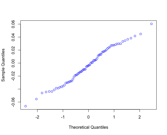
From the above discussion it should be clear that nonparametric modelling of the volatility may provide additional insights for this dataset. We first informally investigated the fact whether an SDE driven by the Wiener process is a suitable model for the data at hand. Many of such models, e.g. the geometric Brownian motion, a classical model for evolution of asset prices over time (also referred to as the Samuelson or Black-Scholes model), rely on an old tenet that returns of asset prices follow a normal distribution. Although the assumption has been empirically disproved for high-frequency financial data (daily or intraday data; see, e.g., [6], [19] and [48]), its violation is less severe for widely spaced data in time (e.g. weekly data, as in our case). In fact, the Shapiro-Wilk test that we performed in R on the returns past the change-point 16 March 1973 did not reject the null hypothesis of normality (-value 0.4). On the other hand, the quantile-quantile (QQ) plot of the same data does perhaps give an indication of a certain mild deviation from normality, see Figure 8, where we also plotted a kernel density estimate of the data (obtained via the command density in R, with bandwidth determined automatically through cross-validation).

In Figure 9 we plot the sample autocorrelation and partial autocorrelation functions based on returns ’s past the change-point 16 March 1973. These do not give decisive evidence against the assumption of independence of ’s. Neither does the Ljung-Box test (the test is implemented in R via the command Box.test), which yields a -value when applied with lags (the -value is certainly small, but not overwhelmingly so).


Summarising our findings, we detected only a mild evidence against the assumption that the returns of the Dow-Jones weekly closings of industrial averages (over the period 16 March 1973 – 2 August 1974, but similar conclusions can be reached also over the other subperiods covered by the DWJ dataset) are approximately independent and follow a normal distribution. Thus there is no strong a priori reason to believe that a geometric Brownian motion is an outright unsuitable model in this setting: it can be used as a first approximation. To account for time-variability of volatility (as suggested by the change-point analysis), we incorporate a time-dependent volatility function in the model, and for additional modelling flexibility we also allow a state-dependent drift. Setting , our model is thus given by
| (14) |
An alternative here is to directly (i.e. without any preliminary transformation) model the Dow-Jones data using equation (1). We consider both possibilities, starting with the model (14).
We used a vague prior on corresponding to the limit , whereas for the other two hyperparameters we assumed . The scaling in the independent Gaussian random walk proposal in the Metropolis-Hastings step was chosen in such a way so as to yield an acceptance rate of ca. . The Gibbs sampler was run for iterations, and the first samples were dropped as a burn-in. We present the estimation results we obtained using and bins, see Figure 10. Although the sample size is quite small in this example, the data are informative enough to yield nontrivial inferential conclusions even with diffuse priors. Both plots in Figure 10 are qualitatively similar and suggest:
- •
A decrease in volatility at the end of 1971, which can be taken as corresponding to the change-point in December 1971 identified in [43]. Unlike that author, we do not directly associate it with suspending the convertibility of the US dollar into gold (that took place in August 1971 rather than December 1971).
- •
A gradual increase in volatility over the subsequent period stretching until the end of 1973. Rather than only the Watergate scandal (and a change-point in March 1973 as in [43]), there could be further economic causes for that, such as the 1973 oil crisis and the 1973–1974 stock market crash.
- •
A decrease in volatility starting in early 1974, compared to the immediately preceding period.
In general, in this work we do not aim at identifying causes for changes in volatility regimes, but prefer to present our inference results, that may subsequently be used in econometric analyses.
Now we move to the Bayesian analysis of the data using model (1). The prior settings were as in the previous case, and we display the results in Figure 11. The overall shapes of the inferred volatility functions are the same in both Figure 10 and Figure 11, and hence similar conclusions apply.
Finally, we stress the fact that our nonparametric Bayesian approach and change-point estimation are different in their scope: whereas our method aims at estimation of the entire volatility function, change-point estimation (as its name actually suggests) concentrates on identifying change-points in the variance of the observed time series, which is a particular feature of the volatility. To that end it assumes the (true) volatility function is piecewise constant, which on the other hand is not an assumption required in our method. Both techniques are useful, and each can provide insights that may be difficult to obtain from another.
5. Conclusions
Bayesian inference for SDEs from discrete-time observations is a difficult task, owing to intractability of the likelihood and the fact that the posterior is not available in closed form. Posterior inference therefore typically requires the use of intricate MCMC samplers. Designing algorithms that result in Markov chains that mix well and explore efficiently the posterior surface is a highly nontrivial problem. Inspired by some ideas from the audio signal processing literature and our earlier work [34], in this paper we introduced a novel nonparametric Bayesian approach to estimation of the volatility coefficient of an SDE. Our method is easy to understand and straightforward to implement via Gibbs sampling, and performs well in practice. Thereby our hope is that our work will contribute to further dissemination and popularisation of a nonparametric Bayesian approach to inference in SDEs, specifically with financial applications in mind. In that respect, see [35], that builds upon the present paper and deals with Bayesian volatility estimation under market microstructure noise. Our work can also be viewed as a partial fulfillment of anticipation in [31] that some ideas developed originally in the context of audio and music processing “will also find use in other areas of science and engineering, such as financial or biomedical data analysis”.
6. Formulae for parameter updates
In this section we present additional details on the derivation of the update formulae for the Gibbs sampler from Section 2. The starting point is to employ the Markov property from (5), and using the standard Bayesian notation, to write the joint density of and as
| (15) |
6.1. Full conditional distributions
We first indicate how (6) was derived. Insert expressions for the individual terms in (15) from (5) and collect separately terms that depend on only, to see that the density of the full conditional distribution of , , is proportional to
Upon normalisation, this expression is the density of the distribution, which proves formula (6). Formula (8) follows directly from the last expression in (5). Formula (9) is proved analogously to (6). Finally, (7) follows from (5) and Bayes’ formula. Cf. also [16], Appendix B.6.
6.2. Metropolis-within-Gibbs step
Now we describe the Metropolis-Hastings step within the Gibbs sampler, that is used to update the hyperparameters of our algorithm, in case the latter are equipped with a prior. For simplicity, assume (we note that such a choice is used in practical examples in [7]), and suppose is equipped with a prior, . Let the hyperparameter be fixed. Obviously, could have been equipped with a prior as well, but this would have further slowed down our estimation procedure, whereas the practical results in Sections 3 and 4 we obtained are already satisfactory with fixed. Using (5) and (15), one sees that the joint density of , and is proportional to
This in turn is proportional to
The latter expression is an unnormalised full conditional density of , and can be used in the Metropolis-within-Gibbs step to update .
The rest of the Metropolis-Hastings step is standard, and the following approach was used in our practical examples: pick a proposal kernel , for instance a Gaussian random walk proposal , where is the density of a normal random variable with mean zero and variance . Note that this specific choice may result in proposing a negative value , which needs to be rejected straightaway as invalid. Then, for computational efficiency, instead of moving to another step within the Gibbs sampler, one keeps on proposing new values until a positive one is proposed. This is then accepted with probability
where is the cumulative distribution function of a normal random variable with mean zero and variance ; otherwise the current value is retained. See [75] for additional details and derivations. Finally, one moves to other steps in the Gibbs sampler, namely to updating ’s and ’s, and iterates the procedure. The acceptance rate in the Metropolis-Hastings step can be controlled through the scale parameter of the proposal density . Some practical rules for determination of an optimal acceptance rate in the Metropolis-Hastings algorithm are given in [28], and those for the Metropolis-within-Gibbs algorithm in [64].
References
- [1] (2007) Modeling with Itô stochastic differential equations. Mathematical Modelling: Theory and Applications, Vol. 22, Springer, Dordrecht. External Links: ISBN 978-1-4020-5952-0, Review MathReviews Cited by: §1.1.
- [2] (2017) Approximate Bayes learning of stochastic differential equations. ArXiv e-prints. External Links: 1702.05390 Cited by: §1.2.
- [3] (2017) Julia: a fresh approach to numerical computing. SIAM Rev. 59 (1), pp. 65–98. External Links: ISSN 0036-1445, Review MathReviews Cited by: §3.
- [4] (2009) Arbitrage theory in continuous time. 3 edition, Oxford University Press. Cited by: §1.1.
- [5] (2017) Variational inference: a review for statisticians. J. Amer. Stat. Assoc. 112 (518), pp. 859–877. Cited by: §2.3.
- [6] (2002) The fine structure of asset returns: an empirical investigation. J. Bus. 75 (2), pp. 305–332. Cited by: §4.
- [7] (2008) Inference and learning in gamma chains for Bayesian audio processing. In Proceedings of Acoustics ’08, pp. 4055–4060. Cited by: §1.3, §2.4, §6.2.
- [8] (2007) Conjugate gamma Markov random fields for modelling nonstationary sources. In Independent Component Analysis and Signal Separation: 7th International Conference, ICA 2007, London, UK, September 9–12, 2007. Proceedings, M. E. Davies, C. J. James, S. A. Abdallah, and M. D. Plumbley (Eds.), pp. 697–705. Cited by: §1.3, §2.2, §2.3, §2.3, §2.4, Remark 1, Remark 2.
- [9] (2007) Variational and stochastic inference for Bayesian source separation. Digit. Signal Process. 17 (5), pp. 891–913. Note: Special Issue on Bayesian Source Separation External Links: ISSN 1051-2004 Cited by: §1.3, §2.3.
- [10] (2012) Parametric statistical change point analysis. 2 edition, Birkhäuser/Springer, New York. Note: With applications to genetics, medicine, and finance External Links: ISBN 978-0-8176-4800-8; 978-0-8176-4801-5, Review MathReviews Cited by: §4, §4.
- [11] (1985) A theory of the term structure of interest rates. Econometrica 53 (2), pp. 385–407. External Links: ISSN 0012-9682, Review MathReviews Cited by: §3.2.
- [12] (2008) Least squares volatility change point estimation for partially observed diffusion processes. Comm. Statist. Theory Methods 37 (13-15), pp. 2342–2357. External Links: ISSN 0361-0926, Review MathReviews Cited by: §4.
- [13] (1977) Maximum likelihood from incomplete data via the EM algorithm. J. Roy. Stat. Soc. B. Met. 39 (1), pp. 1–38. External Links: ISSN 00359246 Cited by: §2.4.
- [14] (1982) Bayesian detection of a change of scale parameter in sequences of independent gamma random variables. J. Econometrics 19 (1), pp. 23–29. External Links: ISSN 0304-4076, Review MathReviews Cited by: §4, §4.
- [15] (2010) Gamma Markov random fields for audio source modeling. IEEE Trans. Audio, Speech, Language Process. 18 (3), pp. 589–601. External Links: ISSN 1558-7916 Cited by: §1.3, §2.4.
- [16] (2008) Inference and parameter estimation in Gamma chains. Technical report Technical Report CUED/F-INFENG/TR.596, University of Cambridge. Cited by: §1.3, §2.4, §6.1.
- [17] (2018) Posterior concentration rates for empirical Bayes procedures with applications to Dirichlet process mixtures. Bernoulli 24 (1), pp. 231–256. External Links: ISSN 1350-7265, Review MathReviews Cited by: §2.4.
- [18] (1995) Adapting to unknown smoothness via wavelet shrinkage. J. Amer. Statist. Assoc. 90 (432), pp. 1200–1224. External Links: ISSN 0162-1459, Review MathReviews Cited by: §3.1, §3.
- [19] (1995) Hyperbolic distributions in finance. Bernoulli 1 (3), pp. 281–299. Cited by: §4.
- [20] (2010) Large-scale inference. Institute of Mathematical Statistics (IMS) Monographs, Vol. 1, Cambridge University Press, Cambridge. Note: Empirical Bayes methods for estimation, testing, and prediction External Links: ISBN 978-0-521-19249-1, Review MathReviews Cited by: §2.4.
- [21] (2001) Likelihood inference for discretely observed nonlinear diffusions. Econometrica 69 (4), pp. 959–993. External Links: ISSN 0012-9682, Review MathReviews Cited by: §1.3.
- [22] (2006) Exact and efficient Bayesian inference for multiple changepoint problems. Stat. Comput. 16 (2), pp. 203–213. External Links: ISSN 0960-3174, Review MathReviews Cited by: §1.3.
- [23] (1951) Diffusion processes in genetics. In Proceedings of the Second Berkeley Symposium on Mathematical Statistics and Probability, 1950, pp. 227–246. External Links: Review MathReviews Cited by: §3.2.
- [24] (1951) Two singular diffusion problems. Ann. of Math. (2) 54, pp. 173–182. External Links: ISSN 0003-486X, Review MathReviews Cited by: §3.2.
- [25] (2013) Inference for diffusion processes. Springer, Heidelberg. Note: With applications in life sciences, With a foreword by Ludwig Fahrmeir External Links: ISBN 978-3-642-25968-5; 978-3-642-25969-2, Review MathReviews Cited by: §1.1, §1.3.
- [26] (1990) Sampling-based approaches to calculating marginal densities. J. Amer. Stat. Assoc. 85 (410), pp. 398–409. Cited by: §2.3.
- [27] (2014) Bayesian data analysis. 3 edition, Texts in Statistical Science Series, CRC Press, Boca Raton, FL. External Links: ISBN 978-1-4398-4095-5, Review MathReviews Cited by: §1.3.
- [28] (1996) Efficient Metropolis jumping rules. In Bayesian statistics, J. M. Bernardo, J. O. Berger, A. P. Dawid, and A. F. M. Smith (Eds.), Vol. 5, pp. 599–607. Cited by: §6.2.
- [29] (1984) Stochastic relaxation, Gibbs distributions, and the Bayesian restoration of images. IEEE Trans. Pattern Anal. Mach. Intell. 6 (6), pp. 721–741. External Links: ISSN 0162-8828 Cited by: §2.3.
- [30] (2017) Fundamentals of nonparametric Bayesian inference. Cambridge Series in Statistical and Probabilistic Mathematics, Vol. 44, Cambridge University Press, Cambridge. External Links: ISBN 978-0-521-87826-5, Review MathReviews Cited by: §5.
- [31] (2007) Bayesian computational methods for sparse audio and music processing. In 15th European Signal Processing Conference (EURASIP), pp. 345–349. Cited by: §5.
- [32] (1995) Reversible jump Markov chain Monte Carlo computation and Bayesian model determination. Biometrika 82 (4), pp. 711–732. External Links: ISSN 0006-3444, Review MathReviews Cited by: §1.3.
- [33] (2003) Trans-dimensional Markov chain Monte Carlo. In Highly structured stochastic systems, Oxford Statist. Sci. Ser., Vol. 27, pp. 179–206. Note: With part A by Simon J. Godsill and part B by Juha Heikkinen External Links: Review MathReviews Cited by: §1.3.
- [34] (2017) Nonparametric Bayesian estimation of a Hölder continuous diffusion coefficient. ArXiv e-prints. External Links: 1706.07449 Cited by: §1.2, §1.3, §1.3, §1.3, §2.1, §2.2, §2.2, §2.4, §3.1, §3.1, §5, §5.
- [35] (2018) Nonparametric Bayesian volatility learning under microstructure noise. ArXiv e-prints. External Links: 1805.05606 Cited by: §5.
- [36] (2014) Consistent non-parametric Bayesian estimation for a time-inhomogeneous Brownian motion. ESAIM Probab. Stat. 18, pp. 332–341. External Links: ISSN 1292-8100, Review MathReviews Cited by: §1.2.
- [37] (2014) Nonparametric Bayesian drift estimation for multidimensional stochastic differential equations. Lith. Math. J. 54 (2), pp. 127–141. External Links: ISSN 0363-1672, Review MathReviews Cited by: §1.2.
- [38] (2016) Posterior contraction rate for non-parametric Bayesian estimation of the dispersion coefficient of a stochastic differential equation. ESAIM Probab. Stat. 20, pp. 143–153. External Links: ISSN 1292-8100, Review MathReviews Cited by: §1.2.
- [39] (1970) Monte Carlo sampling methods using Markov chains and their applications. Biometrika 57 (1), pp. 97–109. External Links: ISSN 0006-3444, Review MathReviews Cited by: §2.4.
- [40] (2011) Empirical dynamics of neuronal rhythms: data-driven modeling of spontaneous magnetoencephalographic and local field potential recordings. Ph.D. Thesis. Cited by: §1.1.
- [41] (1977) Tests for variance shift at an unknown time point. J. R. Stat. Soc. C-App. 26 (3), pp. 279–284. External Links: ISSN 00359254, 14679876 Cited by: §4.
- [42] (1979) Detecting shifts of parameter in gamma sequences with applications to stock price and air traffic flow analysis. J. Amer. Stat. Assoc. 74 (365), pp. 31–40. External Links: ISSN 01621459 Cited by: §4, §4.
- [43] (2008) Simulation and inference for stochastic differential equations. Springer Series in Statistics, Springer, New York. Note: With examples External Links: ISBN 978-0-387-75838-1, Review MathReviews Cited by: 1st item, 2nd item, §4, §4.
- [44] (2016) Sde: simulation and inference for stochastic differential equations. Note: R package version 2.0.15 External Links: Link Cited by: §4.
- [45] (1994) Bayesian analysis of stochastic volatility models. J. Bus. Econ. Stat. 12 (4), pp. 371–389. Cited by: §1.2.
- [46] (2004) Bayesian analysis of stochastic volatility models with fat-tails and correlated errors. J. Econometrics 122 (1), pp. 185–212. External Links: ISSN 0304-4076, Review MathReviews Cited by: §1.2.
- [47] (1991) Brownian motion and stochastic calculus. 2 edition, Graduate Texts in Mathematics, Vol. 113, Springer-Verlag, New York. External Links: ISBN 0-387-97655-8, Review MathReviews Cited by: §1.1.
- [48] (1999) Stock returns and hyperbolic distributions. Math. Comput. Model. 29 (10), pp. 1–15. External Links: ISSN 0895-7177 Cited by: §4.
- [49] (2018) ‘Purposely misspecified’ posterior inference on the volatility of a jump diffusion process. Statist. Probab. Lett. 134 (Supplement C), pp. 106–113. External Links: ISSN 0167-7152 Cited by: §2.1.
- [50] (1953) Equation of state calculations by fast computing machines. J. Chem. Phys. 21 (6), pp. 1087–1092. Cited by: §2.4.
- [51] (2013) Bayesian nonparametric inference—why and how. Bayesian Anal. 8 (2), pp. 269–302. External Links: ISSN 1936-0975, Review MathReviews Cited by: §1.1.
- [52] (2005) Martingale methods in financial modelling. 2 edition, Stochastic Modelling and Applied Probability, Vol. 36, Springer-Verlag, Berlin. External Links: ISBN 3-540-20966-2, Review MathReviews Cited by: §1.1.
- [53] (2012) A Gaussian calculus for inference from high frequency data. Ann. Finance 8 (2-3), pp. 235–258. External Links: ISSN 1614-2446, Review MathReviews Cited by: §2.1, §3.2.
- [54] (2017) Nonparametric Bayesian posterior contraction rates for discretely observed scalar diffusions. Ann. Statist. 45 (4), pp. 1664–1693. External Links: ISSN 0090-5364, Review MathReviews Cited by: §1.2.
- [55] (2012) Nonparametric estimation of diffusions: a differential equations approach. Biometrika 99 (3), pp. 511–531. External Links: ISSN 0006-3444, Review MathReviews Cited by: §1.2.
- [56] (2014) Bayes and empirical Bayes: do they merge?. Biometrika 101 (2), pp. 285–302. External Links: ISSN 0006-3444, Review MathReviews Cited by: §2.4.
- [57] (2013) Posterior consistency via precision operators for Bayesian nonparametric drift estimation in SDEs. Stochastic Process. Appl. 123 (2), pp. 603–628. External Links: ISSN 0304-4149, Review MathReviews Cited by: §1.2.
- [58] (2017) R: a language and environment for statistical computing. R Foundation for Statistical Computing, Vienna, Austria. Cited by: §4.
- [59] (1956) An empirical Bayes approach to statistics. In Proceedings of the Third Berkeley Symposium on Mathematical Statistics and Probability, 1954–1955, vol. I, pp. 157–163. External Links: Review MathReviews Cited by: §2.4.
- [60] (1964) The empirical Bayes approach to statistical decision problems. Ann. Math. Statist. 35, pp. 1–20. External Links: ISSN 0003-4851, Review MathReviews Cited by: §2.4.
- [61] (2004) Monte Carlo statistical methods. 2 edition, Springer Texts in Statistics, Springer-Verlag, New York. External Links: ISBN 0-387-21239-6, Review MathReviews Cited by: §1.3.
- [62] (2001) On inference for partially observed nonlinear diffusion models using the Metropolis-Hastings algorithm. Biometrika 88 (3), pp. 603–621. External Links: ISSN 0006-3444, Review MathReviews Cited by: §1.3.
- [63] (2013) Approximate Gaussian process inference for the drift function in stochastic differential equations. In Advances in Neural Information Processing Systems 26, C. J. C. Burges, L. Bottou, M. Welling, Z. Ghahramani, and K. Q. Weinberger (Eds.), pp. 2040–2048. Cited by: §1.2.
- [64] (2010) The random walk Metropolis: linking theory and practice through a case study. Statist. Sci. 25 (2), pp. 172–190. External Links: ISSN 0883-4237, Review MathReviews Cited by: §6.2.
- [65] (1986) Density estimation for statistics and data analysis. Monographs on Statistics and Applied Probability, Chapman & Hall, London. External Links: ISBN 0-412-24620-1, Review MathReviews Cited by: §1.1.
- [66] (1998) Nonparametric estimation of the diffusion coefficient of a diffusion process. Stochastic Anal. Appl. 16 (1), pp. 185–200. External Links: ISSN 0736-2994, Review MathReviews Cited by: §1.1.
- [67] (1987) The calculation of posterior distributions by data augmentation. J. Amer. Statist. Assoc. 82 (398), pp. 528–550. Note: With discussion and with a reply by the authors External Links: ISSN 0162-1459, Review MathReviews Cited by: §1.3.
- [68] (1994) Markov chains for exploring posterior distributions. Ann. Statist. 22 (4), pp. 1701–1762. Note: With discussion and a rejoinder by the author External Links: ISSN 0090-5364, Review MathReviews Cited by: §2.4.
- [69] (2014) Reversible jump MCMC for nonparametric drift estimation for diffusion processes. Comput. Statist. Data Anal. 71, pp. 615–632. External Links: ISSN 0167-9473, Review MathReviews Cited by: §1.2.
- [70] (2017) Bayesian estimation of discretely observed multi-dimensional diffusion processes using guided proposals. Electron. J. Stat. 11 (1), pp. 2358–2396. External Links: ISSN 1935-7524, Review MathReviews Cited by: §1.3.
- [71] (2013) Consistent nonparametric Bayesian inference for discretely observed scalar diffusions. Bernoulli 19 (1), pp. 44–63. External Links: ISSN 1350-7265, Review MathReviews Cited by: §1.2.
- [72] (2013) Nonparametric Bayesian methods for one-dimensional diffusion models. Math. Biosci. 243 (2), pp. 215–222. External Links: ISSN 0025-5564, Review MathReviews Cited by: §1.2.
- [73] (2008) Bayesian extensions to non-negative matrix factorisation for audio signal modelling. In 2008 IEEE International Conference on Acoustics, Speech and Signal Processing, pp. 1825–1828. Cited by: §1.3.
- [74] (2006) All of nonparametric statistics. Springer Texts in Statistics, Springer, New York. External Links: ISBN 978-0387-25145-5; 0-387-25145-6, Review MathReviews Cited by: §3.1.
- [75] (2012) Metropolis Hastings MCMC when the proposal and target have differing support. Blog. Note: Online; accessed on 23 December 2017 External Links: Link Cited by: §6.2.
- [76] (1985) Stochastic processes in engineering systems. Springer Texts in Electrical Engineering, Springer-Verlag, New York. External Links: ISBN 0-387-96061-9, Review MathReviews Cited by: §1.1.
- [77] (2001) Bayesian binary segmentation procedure for a Poisson process with multiple changepoints. J. Comput. Graph. Statist. 10 (4), pp. 772–785. External Links: ISSN 1061-8600, Review MathReviews Cited by: §1.3.